Complete Solutions and Triality Theory to a Nonconvex Optimization Problem with Double-Well Potential in ${I\!\!R}^{n}$

Abstract

The main purpose of this research note is to show that the triality theory can always be used to identify both global minimizer and the biggest local maximizer in global optimization. An open problem left on the double-min duality is solved for a nonconvex optimization problem with double-well potential in ${I\!\!R}^{n}$, which leads to a complete set of analytical solutions. Also a convergency theorem is proved for linear perturbation canonical dual method, which can be used for solving global optimization problems with multiple solutions. The methods and results presented in this note pave the way towards the proof of the triality theory in general cases.

1 Primal Problem and Motivation

We are interested in analytical solutions to the following global minimization problem ($({\cal{P}})$ in short):

$$({\cal{P}}):\;\;\;\min\{\Pi(x)=W(x)-\langle x,f\rangle\;|\;\;x\in{I\!\!R}^{n}\},$$ (1)

where $f\in{I\!\!R}^{n}$ is a given vector, $\langle x,f\rangle$ represents the inner product in ${I\!\!R}^{n}$, and $W:{I\!\!R}^{n}\rightarrow{I\!\!R}$ is a fourth order polynomial of the form

$$W(x):=\frac{{\alpha}}{2}\left(\frac{1}{2}|x|^{2}-\lambda\right)^{2},$$

in which, ${\alpha}$ and $\lambda$ are given positive parameters.

(a) Function $\Pi$ when $n,f,{\alpha}=1$ and ${\lambda}=3$.

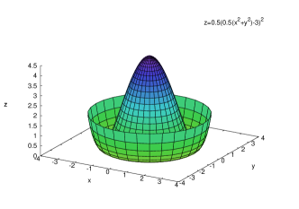
(b) Function $\Pi$ when $n=2$, $f=0$, ${\alpha}=1$ and ${\lambda}=3$.

Figure 1: Graphs of $\Pi(x)$

The non-convex problem $({\cal{P}})$ appears extensively in many applications of sciences and engineering. For example, in the case that $n=1$, $\Pi(x)$ is a double-well function (see figure 1a), which was first studied by van der Waals in thermal mechanics in 1895. If $n=2$ and $f=0$ this is the so-called Mexican hat function (see Figure 1b) in cosmology and theoretical physics. Due to the nonconvexity, the function $\Pi(x)$ may possess multiple critical points, determined by the necessary condition

$$\nabla\Pi(x)={\alpha}\left(\frac{1}{2}|x|^{2}-{\lambda}\right)x-f=0.$$

Direct methods for solving this nonlinear algebraic equation are difficult, and to identify the global minimizer is a main task in global optimization.

If instead of the function $W$ considered above, we were to consider the function $W_{B}:{I\!\!R}^{n}\rightarrow{I\!\!R}$ defined by

$$W_{B}(x):=\frac{{\alpha}}{2}\left(\frac{1}{2}|Bx|^{2}-\lambda\right)^{2},$$

where $B:{I\!\!R}^{n}\rightarrow{I\!\!R}^{m}$ is a linear transformation (not identically zero), now the function $\Pi(x)=W_{B}(x)-\langle f,x\rangle$ gives a more general case for problem $(P)$. Yet, if we take $f\in R(B^{t}B)$, we can always reduce $(P)$ to the case where $B=I$ in the following way: make $y=Bx$ and let $\overline{f}=B(B^{t}B)^{\dagger}f$, where $(B^{t}B)^{\dagger}$ is the Moore-Penrose pseudoinverse of $B^{t}B$ (see [2], [12] and references therein). Notice that since $f\in R(B^{t}B)$ then $B^{t}\overline{f}=f$ and

$$\langle f,x\rangle=\langle B^{t}\overline{f},x\rangle=\langle\overline{f},Bx\rangle=\langle\overline{f},y\rangle.$$

With this, we can define the function $\Pi_{B}:R(B)\rightarrow{I\!\!R}$ where

$$\Pi_{B}(y)=\frac{{\alpha}}{2}\left(\frac{1}{2}|y|^{2}-\lambda\right)^{2}-\langle\overline{f},y\rangle.$$

If $y_{0}\in R(B)$ is a solution of $\Pi_{B}$, there must exist a $x_{0}\in{I\!\!R}^{n}$ such that $Bx_{0}=y_{0}$, then

$$B^{t}Bx_{0}=B^{t}y_{0}$$

and from this, we can take $x_{0}=(B^{t}B)^{\dagger}B^{t}y_{0}$ as a solution for $\Pi$. Thanks to this, we will study only the case when $B=I$.

Canonical duality theory developed in [3] is potentially powerful for solving a large class of nonconvex/nonsmooth/discrete problems in both analysis and global optimization [7, 8, 9]. This theory is composed mainly of (a) a canonical dual transformation, (b) a complementary-dual principle, and (c) a triality theory. It was shown in [4] that by the canonical dual transformation, the fourth-order nonconvex problem $({\cal{P}})$ is equivalent to an one-dimensional canonical dual problem which can be solved analytically to obtain all critical points. The complementary-dual principle shows that a complete set of solutions to the primal problem can be represented analytically by these canonical dual solutions. By the triality theory, both global minimizer and local maximizer can be identified. However, it was discovered in 2003 that in order to identify local minimizer, the triality theory proposed in [3] needs “certain additional constraints” (see Remark 1 in [4]). Therefore, the double-min duality statement in this triality theory was left as an open problem in global optimization [5].

The canonical duality theory and the associated triality have been challenged recently by Voisei and Z$\breve{a}$linescua in a set of more than seven papers. Unfortunately, in these papers, they either made mistakes in understanding some basic terminologies of finite deformation mechanics, or repeatedly address the same type of open problem for the double-min duality left unaddressed by Gao in [4, 5]. For example, the external energy $F(u)$ in conservative systems (the case studied by Gao and Strang in [10]) means that the gradient $\nabla F(u)$ must be a given external force field. Therefore, the function(al) $F(u)$ in Gao and Strang’s work can not be quadratic. However, in their paper published recently in Applicable Analysis, quadratic $F(u)$ has been used by Voisei and Z$\breve{a}$linescua in all “counterexamples”. Also, interested readers should find that the references [4, 5], where the open problem was remarked, never been cited in any one of their papers.

The main purpose of this paper is to solve this open problem such that the proposed problem $({\cal{P}})$ can be solved completely. The method and results presented in this paper have been used to prove the triality theory for global optimization problems with general polynomials [11] and general objective functions [13, 15].

2 Canonical Dual Problem and Analytical Solutions

Following the standard procedure of the canonical dual transformation, first we need to choose a geometric operator ${\Lambda}:{I\!\!R}^{n}\rightarrow[-{\lambda},+\infty)$ given by the following function

$${\Lambda}(x)=\frac{1}{2}|x|^{2}-{\lambda},$$

and the associated canonical function $V:[-{\lambda},+\infty)\rightarrow{I\!\!R}_{+}$ defined by

$$V(\xi)=\frac{{\alpha}}{2}\xi^{2}.$$

Therefore, the primal function $\Pi$ can be reformulated as

$$\Pi(x)=V({\Lambda}(x))-\langle f,x\rangle.$$

By the Legendre transformation (see [1, 17, 19]), the conjugate function $V^{c}:[-{\alpha}{\lambda},+\infty)\rightarrow{I\!\!R}_{+}$ is given by

$$V^{c}(\varsigma)=\frac{\varsigma^{2}}{2{\alpha}}.$$

With this, the Gao-Strang total complementary function $\Xi:{I\!\!R}^{n}\times[-{\alpha}{\lambda},+\infty)\rightarrow{I\!\!R}$, associated to the problem $({\cal{P}})$ can be defined as follows:

$$\Xi(x,\varsigma)=\varsigma{\Lambda}(x)-\frac{\varsigma^{2}}{2{\alpha}}-\langle f,x\rangle.$$

Via this $\Xi(x,\varsigma)$, the canonical dual function $\Pi^{d}:[-{\alpha}{\lambda},+\infty)\rightarrow{I\!\!R}$ can be finally obtained by [4]

$$\Pi^{d}(\varsigma) := {{\rm sta}}_{{}_{{}_{{}_{{{x}}\in{I\!\!R}^{n}}}}}\Xi(x,\varsigma)=\{\Xi(x_{0},\varsigma)|\;\;\nabla_{x}\Xi(x_{0},\varsigma)=0\}$$

$$= -\frac{|f|^{2}}{2\varsigma}-\frac{\varsigma^{2}}{2{\alpha}}-\varsigma{\lambda},\ \forall\varsigma\in[-{\alpha}{\lambda},+\infty),$$

where the notation ${\rm sta}\{*\}$ stands for finding stationary points of the function given in $\{*\}$.

Notice that if $\varsigma>0$ then the dual function $\Pi^{d}(\varsigma)$ is strictly concave which admits a unique global maximizer; however, $\Pi^{d}(\varsigma)$ is a d.c. function (difference of convex functions) on $[-{\alpha}{\lambda},0)$, which should give us information about local extrema of the primal function $\Pi$. Therefore, the canonical dual problem is proposed in the following stationary form:

$$({\cal{P}}^{d}):\;\;\;{{\rm sta}}_{{}_{{}_{{}_{\varsigma\in[-{\alpha}{\lambda},+\infty)}}}}\Pi^{d}(\varsigma)=\{\Pi^{d}(\varsigma_{o})|\nabla\Pi^{d}(\varsigma_{o})=0\}.$$ (2)

By the fact that the canonical dual problem $({\cal{P}}^{d})$ has only one variable, the criticality condition $\nabla\Pi^{d}(\varsigma)=0$, where

$$\nabla\Pi^{d}(\varsigma)=\frac{|f|^{2}}{2\varsigma^{2}}-\frac{\varsigma}{{\alpha}}-{\lambda},$$ (3)

leads to a quebec algebraic equation

$$2\varsigma^{2}\left(\frac{\varsigma}{{\alpha}}+{\lambda}\right)=|f|^{2},$$ (4)

which can be solved explicitly to obtain all three possible real solutions:

$$\varsigma_{1} = r^{1/3}+\frac{{\alpha}^{2}\cdot{\lambda}^{2}}{9r^{1/3}}-\frac{{\alpha}\cdot{\lambda}}{3}$$ (5)

$$\varsigma_{2} = \left(-\frac{\sqrt{3}\,i}{2}-\frac{1}{2}\right)\cdot r^{1/3}+\frac{\left(\frac{\sqrt{3}\,i}{2}-\frac{1}{2}\right)\cdot{\alpha}^{2}\cdot{\lambda}^{2}}{9r^{1/3}}-\frac{{\alpha}\cdot{\lambda}}{3}$$ (6)

$$\varsigma_{3} = \left(\frac{\sqrt{3}\,i}{2}-\frac{1}{2}\right)\cdot r^{1/3}+\frac{\left(-\frac{\sqrt{3}\,i}{2}-\frac{1}{2}\right)\cdot{\alpha}^{2}\cdot{\lambda}^{2}}{9r^{1/3}}-\frac{{\alpha}\cdot{\lambda}}{3},$$ (7)

where

$$r=\frac{{\alpha}\cdot|f|\,\sqrt{27\,{|f|}^{2}-8\,{{\alpha}}^{2}\cdot{{\lambda}}^{3}}}{4\cdot{3}^{\frac{3}{2}}}+\frac{27\,{{\alpha}}\cdot{|f|}^{2}-4\,{{\alpha}}^{3}\cdot{{\lambda}}^{3}}{108}.$$

It is not difficult to show that if $|f|^{2}>8{\alpha}^{2}{\lambda}^{3}/27$ then $\varsigma_{1}$ is the only real positive root and if $|f|^{2}=8{\alpha}^{2}{\lambda}^{3}/27$ then $\varsigma_{1}$ is positive, and $\varsigma_{2}=\varsigma_{3}=-2{\alpha}{\lambda}/3$. If $0<|f|^{2}<8{\alpha}^{2}{\lambda}^{3}/27$, equations (5)-(7) can be simplified further to obtain:

$$\varsigma_{1} = \frac{{\alpha}{\lambda}}{3}\left(2\cos\left(\frac{1}{3}\cos^{-1}\left(\frac{27|f|^{2}}{4{\alpha}^{2}{\lambda}^{3}}-1\right)\right)-1\right)$$ (8)

$$\varsigma_{2} = \frac{{\alpha}{\lambda}}{3}\left(2\cos\left(\frac{1}{3}\cos^{-1}\left(\frac{27|f|^{2}}{4{\alpha}^{2}{\lambda}^{3}}-1\right)+\frac{4\pi}{3}\right)-1\right)$$ (9)

$$\varsigma_{3} = \frac{{\alpha}{\lambda}}{3}\left(2\cos\left(\frac{1}{3}\cos^{-1}\left(\frac{27|f|^{2}}{4{\alpha}^{2}{\lambda}^{3}}-1\right)+\frac{2\pi}{3}\right)-1\right).$$ (10)

Moreover, we will have that $\varsigma_{1}>0>\varsigma_{2}>-2{\alpha}{\lambda}/3>\varsigma_{3}>-{\alpha}{\lambda}$.

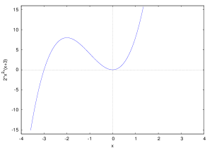
Figure 2: The function $2\varsigma^{2}(\varsigma+{\alpha}{\lambda})$ with ${\alpha}{\lambda}=3$.

Theorem 1 (Analytical Solutions [4])

Let $f\in{I\!\!R}^{n}\setminus\{0\}$ and $\{\varsigma_{i}\}$ be the real roots of Equation (4). Then, $x_{i}=f/\varsigma_{i}$ are stationary points of $(P)$ for every $i$ and $\Pi(x_{i})=\Pi^{d}(\varsigma_{i})$.

Proof: Notice that ${\Lambda}(x_{i})=\varsigma_{i}/{\alpha}$, we have

$${\Lambda}(x_{i})=\frac{1}{2}|x_{i}|^{2}-{\lambda}=\frac{|f|^{2}}{2\varsigma_{i}^{2}}-{\lambda}$$

but since $\varsigma_{i}$ is solution of (4), we have

$${\Lambda}(x_{i})=\left(\frac{\varsigma_{i}}{{\alpha}}+{\lambda}\right)-{\lambda}=\frac{\varsigma_{i}}{{\alpha}}.$$ (11)

Now, if we differentiate the function $\Pi$ we will have

$$\nabla\Pi(x)={\alpha}{\Lambda}(x)x-f$$ (12)

and so

$$\nabla\Pi(x_{i})={\alpha}{\Lambda}(x_{i})x_{i}-f={\alpha}\cdot\frac{\varsigma_{i}}{{\alpha}}\cdot\frac{f}{\varsigma_{i}}-f=0.$$

On the other hand

$$\Pi(x_{i})=\frac{{\alpha}}{2}\cdot\frac{\varsigma_{i}^{2}}{{\alpha}^{2}}-\frac{|f|^{2}}{\varsigma_{i}}=\frac{\varsigma_{i}^{2}}{2{\alpha}}-\left(\frac{2\varsigma_{i}^{2}}{{\alpha}}+2\varsigma_{i}{\lambda}\right)=-\frac{3\varsigma_{i}^{2}}{2{\alpha}}-2\varsigma_{i}{\lambda}$$

and

$$\Pi^{d}(\varsigma_{i})=-\frac{|f|^{2}}{2\varsigma_{i}}-\frac{\varsigma_{i}^{2}}{2{\alpha}}-\varsigma_{i}{\lambda}=-\left(\frac{\varsigma_{i}^{2}}{{\alpha}}+\varsigma_{i}{\lambda}\right)-\frac{\varsigma_{i}^{2}}{2{\alpha}}-\varsigma_{i}{\lambda}=-\frac{3\varsigma_{i}^{2}}{2{\alpha}}-2\varsigma_{i}{\lambda},$$

so we have $\Pi(x_{i})=\Pi^{d}(\varsigma_{i})$ as expected. $\blacksquare$

Theorem 1 shows that the stationary points of the dual problem induce naturally stationary points of the primal with zero duality gap. Using (12), it can be seen that if any stationary point of $\Pi$ exists, it must be in the same direction of $f$. Therefore, by analyzing the function $W(rf)$ with $r\in{I\!\!R}$ it can be seen that the possible stationary points of $W(rf)$ satisfy the following equation:

$${\alpha}r\left(\frac{r^{2}}{2}|f|^{2}-{\lambda}\right)=1.$$ (13)

Since $f\neq 0$, then $r\neq 0$ and by substituting $r=1/\varsigma$ in (13) we will have (4). Thus, problem $({\cal{P}})$ has at most three critical points. In the next section, we will show that the extremality of these solutions can be identified by a refined triality theory.

3 Triality Theory and Perturbation

The following spaces are important for understanding the triality theory:

$${\cal X}_{\sharp} := \left\{x\in{I\!\!R}^{n}|\;\;\left|\frac{\langle f,x\rangle}{|f||x|}\right|<\sqrt{-\frac{\varsigma_{2}}{2\varsigma_{2}+2{\alpha}{\lambda}}}\right\},$$ (14)

$${\cal X}_{\flat} := \left\{x\in{I\!\!R}^{n}|\;\;\left|\frac{\langle f,x\rangle}{|f||x|}\right|>\sqrt{-\frac{\varsigma_{2}}{2\varsigma_{2}+2{\alpha}{\lambda}}}\right\}.$$ (15)

Theorem 2 (Refined Triality Theory)

Let $f\in{I\!\!R}^{n}$ be a given vector such that $0<|f|^{2}<8{\alpha}^{2}{\lambda}^{3}/27$, $\{\varsigma_{i}\}$ with $i=1,2,3$ the three real roots of Equation (4) such that $\varsigma_{1}>0>\varsigma_{2}>-2{\alpha}{\lambda}/3>\varsigma_{3}>-{\alpha}{\lambda}$ and let $x_{i}=f/\varsigma_{i}$. Then we have

1. $x_{1}$ is a global minimizer of $\Pi$, $\varsigma_{1}$ is a maximizer of $\Pi^{d}$ in $(0,+\infty)$, and

   $$\Pi(x_{1})=\min_{x\in{I\!\!R}^{n}}\Pi(x)=\max_{\varsigma\in(0,+\infty)}\Pi^{d}(\varsigma)=\Pi^{d}(\varsigma_{1}).$$ (16)

2. There exist ${\cal X}_{o}$ and $I_{o}$ neighborhoods of $x_{3}$ and $\varsigma_{3}$ respectively such that $x_{3}$ is a local maximizer of $\Pi(x)$ in ${\cal X}_{o}$ and $\varsigma_{3}$ is a local maximizer of $\Pi^{d}(\varsigma)$ in $I_{o}$, and

   $$\Pi(x_{3})=\max_{x\in{\cal X}_{o}}\Pi(x)=\max_{\varsigma\in I_{o}}\Pi^{d}(\varsigma)=\Pi^{d}(\varsigma_{3}).$$ (17)

3. There exists $I_{1}$ a neighborhood of $\varsigma_{2}$ such that $\varsigma_{2}$ is a local minimizer of $\Pi^{d}(\varsigma)$ in $I_{1}$ and $x_{2}$ is a saddle point of $\Pi(x)$. Specifically, $x_{2}$ is a local maximizer of $\Pi(x)$ in the directions $x_{2}+t{\cal X}_{\sharp}$ and a local minimizer of $\Pi(x)$ in the directions $x_{2}+t{\cal X}_{\flat}$, i.e.,

   $$\Pi(x_{2})=\max_{t\in{I\!\!R}}\Pi(x_{2}+t{\cal X}_{\sharp})=\min_{\varsigma\in I_{1}}\Pi^{d}(\varsigma)=\Pi^{d}(\varsigma_{2}),$$ (18)

   $$\Pi(x_{2})=\min_{t\in{I\!\!R}}\Pi(x_{2}+t{\cal X}_{\flat})=\min_{\varsigma\in I_{1}}\Pi^{d}(\varsigma)=\Pi^{d}(\varsigma_{2}).$$ (19)

Proof:

1. The canonical dual solution $\varsigma_{1}$ is a global minimizer of $\Pi^{d}$ in $(0,+\infty)$ since $\Pi^{d}$ is a strictly concave function and $\varsigma_{1}$ is its only critical point in $(0,+\infty)$. Since $\varsigma_{1}>0$, $\Xi(\cdot,\varsigma_{1})$ is a strictly convex function, then its only minimizer happens at its stationary point which is $x_{1}$. Also, $\Xi(x,\varsigma_{1})\leq\Pi(x)$ for every $x$; in fact, since $V$ is a strictly convex function, by Fenchel’s inequality for Convex functions we have that for every $\varsigma$ and every $\xi$

   $$\varsigma\cdot\xi\leq V(\xi)+V^{c}(\varsigma).$$

   Taking $\varsigma=\varsigma_{1}$ and $\xi={\Lambda}(x)$

   $$\varsigma_{1}{\Lambda}(x)\leq V({\Lambda}(x))+V^{c}(\varsigma_{1}),$$

   rearranging the last inequality and adding $-\langle f,x\rangle$ to both sides we have $\Xi(x,\varsigma_{1})\leq\Pi(x)$ for every $x\in{I\!\!R}^{n}$.
   

   Using Equation (11), ${\Lambda}(x_{1})=\varsigma_{1}/{\alpha}$, it can be easily shown that $\Pi(x_{1})=\Xi(x_{1},\varsigma_{1})$. With this, assume that there exists $x^{\prime}\in{I\!\!R}^{n}$ such that $\Pi(x_{1})>\Pi(x^{\prime})$ then

   $$\Pi(x_{1})>\Pi(x^{\prime})\geq\Xi(x^{\prime},\varsigma_{1})\geq\Xi(x_{1},\varsigma_{1})=\Pi(x_{1})$$

   which is a contradiction. Therefore $x_{1}$ is a solution of $(P)$.

2. By the second derivative of $\Pi^{d}$, we have:

   $$\nabla^{2}\Pi^{d}(\varsigma)=-\frac{|f|^{2}}{\varsigma^{3}}-\frac{1}{{\alpha}}.$$

   Then

   $$\nabla^{2}\Pi^{d}(\varsigma_{i}) = -\frac{|f|^{2}}{\varsigma_{i}^{3}}-\frac{1}{{\alpha}}=-\frac{2}{\varsigma_{i}}\left(\frac{\varsigma_{i}}{{\alpha}}+{\lambda}\right)-\frac{1}{{\alpha}}$$ (20)

   $$= -\frac{2}{{\alpha}}-\frac{2{\lambda}}{\varsigma_{i}}-\frac{1}{{\alpha}}=\frac{3\varsigma_{i}+2{\alpha}{\lambda}}{-{\alpha}\varsigma_{i}}.$$

   For $i=3$, $\nabla^{2}\Pi^{d}(\varsigma_{3})<0$ and $\varsigma_{3}$ is a local maximizer of $\Pi^{d}$.
   

   On the other hand, by differentiating (12) we have:

   $$\nabla^{2}\Pi(x)={\alpha}\left(xx^{t}+{\Lambda}(x)I\right)$$

   and

   $$\nabla^{2}\Pi(x_{i})={\alpha}\left(x_{i}x^{t}_{i}+{\Lambda}(x_{i})I\right)={\alpha}\left(\frac{ff^{t}}{\varsigma_{i}^{2}}+\frac{\varsigma_{i}}{{\alpha}}I\right).$$

   For $i=3$, take any $z\in{I\!\!R}^{n}$:

   $$z^{t}\nabla^{2}\Pi(x_{3})z={\alpha}\left(\frac{z^{t}ff^{t}z}{\varsigma_{3}^{2}}+\frac{\varsigma_{3}}{{\alpha}}|z|^{2}\right)={\alpha}\left(\frac{\langle f,z\rangle^{2}}{\varsigma_{3}^{2}}+\frac{\varsigma_{3}}{{\alpha}}|z|^{2}\right),$$

   therefore, by the Cauchy-Schwarz inequality we have

   $$z^{t}\nabla^{2}\Pi(x_{3})z \leq {\alpha}\left(\frac{|f|^{2}|z|^{2}}{\varsigma_{3}^{2}}+\frac{\varsigma_{3}}{{\alpha}}|z|^{2}\right)={\alpha}\cdot|z|^{2}\left(\frac{|f|^{2}}{\varsigma_{3}^{2}}+\frac{\varsigma_{3}}{{\alpha}}\right)$$ (21)

   $$= {\alpha}\cdot|z|^{2}\left(\frac{3\varsigma_{3}}{{\alpha}}+2{\lambda}\right).$$

   But the expression in brackets is negative so $z^{t}\nabla^{2}\Pi(x_{3})z\leq 0$ for every $z\in{I\!\!R}^{n}$ and $\Pi$ has a local maximizer at $x_{3}$.

3. Using Equation (20) with $i=2$, we have that $\nabla^{2}\Pi^{d}(\varsigma_{2})>0$ and $\varsigma_{2}$ is a local minimizer of $\Pi^{d}$.
   

   On the other hand, by taking $z\in{I\!\!R}^{n}$, we know that $\phi(t)=\Pi(x_{2}+tz)$ has first and second derivatives as follows:

   $$\phi^{\prime}(t)=\nabla\Pi(x_{2}+tz)z,\quad\phi^{\prime\prime}(t)=z^{t}\nabla^{2}\Pi(x_{2}+tz)z.$$

   Clearly, $\phi^{\prime}(0)=0$. What about $\phi^{\prime\prime}(0)$?
   
   Consider $\theta$ the angle between $z$ and $f$. Then

   $$\phi^{\prime\prime}(0)=z^{t}\nabla^{2}\Pi(x_{2})z={\alpha}\left(\frac{\langle f,z\rangle^{2}}{\varsigma_{2}^{2}}+\frac{\varsigma_{2}}{{\alpha}}|z|^{2}\right)={\alpha}\left(\frac{|f|^{2}|z|^{2}\cos^{2}\theta}{\varsigma_{2}^{2}}+\frac{\varsigma_{2}}{{\alpha}}|z|^{2}\right)$$

   $$={\alpha}|z|^{2}\left(\frac{|f|^{2}}{\varsigma_{2}^{2}}\cos^{2}\theta+\frac{\varsigma_{2}}{{\alpha}}\right)={\alpha}|z|^{2}\left(\left(\frac{2\varsigma_{2}}{{\alpha}}+2{\lambda}\right)\cos^{2}\theta+\frac{\varsigma_{2}}{{\alpha}}\right),$$

   so

   $$\phi^{\prime\prime}(0)=|z|^{2}\left((2\varsigma_{2}+2{\alpha}{\lambda})\cos^{2}\theta+\varsigma_{2}\right).$$ (22)

   If $z\in{\cal X}_{\sharp}$, by the definition of ${\cal X}_{\sharp}$, we have that

   $$|\cos\theta|=\left|\frac{\langle f,x\rangle}{|f||x|}\right|<\sqrt{-\frac{\varsigma_{2}}{2\varsigma_{2}+2{\alpha}{\lambda}}}.$$

   Then

   $$\cos^{2}\theta<-\frac{\varsigma_{2}}{2\varsigma_{2}+2{\alpha}{\lambda}}$$

   $$(2\varsigma_{2}+2{\alpha}{\lambda})\cos^{2}\theta<-\varsigma_{2}$$

   $$(2\varsigma_{2}+2{\alpha}{\lambda})\cos^{2}\theta+\varsigma_{2}<0.$$ (23)

   So, substituting (23) into (22) implies that, $\phi^{\prime\prime}(0)<0$ and $t=0$ is a local maximizer.
   

   If $z\in{\cal X}_{\flat}$, then by definition, we have

   $$\sqrt{-\frac{\varsigma_{2}}{2\varsigma_{2}+2{\alpha}{\lambda}}}<\left|\frac{\langle f,x\rangle}{|f||x|}\right|=|\cos\theta|.$$

   Then

   $$-\frac{\varsigma_{2}}{2\varsigma_{2}+2{\alpha}{\lambda}}<\cos^{2}\theta,$$

   and this implies that

   $$0<(2\varsigma_{2}+2{\alpha}{\lambda})\cos^{2}\theta+\varsigma_{2}.$$ (24)

   Thus, from the equation (22) we know that $\phi^{\prime\prime}(0)>0$ and $t=0$ is a local minimizer. $\blacksquare$

Remark 1: The triality theory says precisely that if $\varsigma_{1}$ is a global maximizer of $\Pi^{d}$ on a certain set, then $x_{1}$ is a global minimizer for $\Pi$. This is known from the general result by Gao and Strang in [10]. If $\varsigma_{3}$ is a local maximizer for $\Pi^{d}$ then $x_{3}$ is also a local maximizer for $\Pi$. This is the so-called double-max duality statement. If $\varsigma_{2}$ is a local minimizer for $\Pi^{d}$, then $x_{2}$ is also a local minimizer for $\Pi$ in certain directions. This is so-called double-min duality in the standard triality form proposed in [3]. The “certain additional constraint” discovered in [4, 5] is $x=x_{2}+t{\cal X}_{\flat}\;\;\forall t\in{I\!\!R}$. Part iii of Theorem 2 is showing that $x_{2}$ is, in fact, a saddle point. This solves the open problem left in [4, 5] for this special case of double-well potential problem.
Remark 2: If $|f|^{2}=8{\alpha}^{2}{\lambda}^{3}/27$, then $\varsigma_{2}=\varsigma_{3}=-2{\alpha}{\lambda}/3$ and Equation (20) implies that $\nabla^{2}\Pi^{d}(-2{\alpha}{\lambda}/3)=0$, even more, it is not hard to show that this is an inflexion point of $\Pi^{d}$. The triality theory in this case can not tell us what kind of stationary point is for $x_{2}$. However, Equation (21) remains true, and in this case (recall that $x_{3}=x_{2}$) the expression in brackets is zero. So this implies that $z^{t}\nabla^{2}\Pi(x_{2})z\leq 0$ for every $z\in{I\!\!R}^{n}$ and $x_{2}$ is a local maximizer of $\Pi$.

It is clear that if $f=0$, the problem $({\cal{P}})$ has infinite number of global minimizers, they all lie in the sphere $|x|^{2}=2{\lambda}$. In this case, the canonical dual is strictly concave with only one local maximizer $\varsigma_{2}$, which leads to a local maximizer $x=0$ of the primal problem. Therefore, a linear perturbation method has been introduced in [16] for solving some NP-hard problems in global optimization. The next theorem proves the convergence of this canonical dual perturbation method under the current setting. Notice that we want to find at least a solution of $({\cal{P}})$ if $f=0$.

Theorem 3

Consider $({\cal{P}})$ with $f=0$. Let ${\alpha},{\lambda}\in{I\!\!R}^{+}$, $f_{o}\in{I\!\!R}^{n}$ such that $0<|f_{o}|^{2}<8{\alpha}^{2}{\lambda}^{3}/27$ and consider $f_{k}=f_{o}/k,$ for every $k\in I\!\!N$. For $i=1,2,3$, take $\varsigma_{i,k}$ the critical points of $\Pi_{k}^{d}$ which is the dual function induced by $\Pi_{k}(x)=W(x)-\langle x,f_{k}\rangle$, and $x_{i,k}=f_{k}/\varsigma_{i,k}$. Then

$$\lim_{k\rightarrow\infty}x_{1,k}=\overline{x}_{1}\text{ and }|\overline{x}_{1}|^{2}=2{\lambda},$$

$$\lim_{k\rightarrow\infty}x_{2,k}=\overline{x}_{2}\text{ and }|\overline{x}_{2}|^{2}=2{\lambda},$$

$$\lim_{k\rightarrow\infty}x_{3,k}=0.$$

Proof: Since $x_{i,k}=f_{k}/\varsigma_{i,k}=f_{o}/(k\varsigma_{i,k})$ we need to show that $1/(k\varsigma_{i,k})$ converges for every $i$. Since $f_{k}$ is converging to zero, from equations (8)-(10), we can see that $\varsigma_{1,k}$ and $\varsigma_{2,k}$ both converge to zero and $\varsigma_{3,k}$ converges to $-{\alpha}{\lambda}$. Thanks to (4) we know that

$$2\left(\frac{\varsigma_{i,k}}{{\alpha}}+{\lambda}\right)=\frac{|f_{k}|^{2}}{(\varsigma_{i,k})^{2}}=\frac{|f_{o}|^{2}}{(k\varsigma_{i,k})^{2}},$$

which implies that

$$\frac{1}{k|\varsigma_{i,k}|}=\frac{\sqrt{2\left(\frac{\varsigma_{i,k}}{{\alpha}}+{\lambda}\right)}}{|f_{o}|}.$$

With this, we have:

$$\lim_{k\rightarrow\infty}\frac{1}{k|\varsigma_{1,k}|}=\lim_{k\rightarrow\infty}\frac{1}{k\varsigma_{1,k}}=\lim_{k\rightarrow\infty}\frac{\sqrt{2\left(\frac{\varsigma_{1,k}}{{\alpha}}+{\lambda}\right)}}{|f_{o}|}=\frac{\sqrt{2{\lambda}}}{|f_{o}|},$$

$$\lim_{k\rightarrow\infty}\frac{1}{k|\varsigma_{2,k}|}=-\lim_{k\rightarrow\infty}\frac{1}{k\varsigma_{2,k}}=\lim_{k\rightarrow\infty}\frac{\sqrt{2\left(\frac{\varsigma_{2,k}}{{\alpha}}+{\lambda}\right)}}{|f_{o}|}=\frac{\sqrt{2{\lambda}}}{|f_{o}|},$$

and

$$\lim_{k\rightarrow\infty}\frac{1}{k|\varsigma_{3,k}|}=-\lim_{k\rightarrow\infty}\frac{1}{k\varsigma_{3,k}}=\lim_{k\rightarrow\infty}\frac{\sqrt{2\left(\frac{\varsigma_{3,k}}{{\alpha}}+{\lambda}\right)}}{|f_{o}|}=\frac{0}{|f_{o}|}=0.$$

Finally, we have

$$\lim_{k\rightarrow\infty}x_{1,k}=\lim_{k\rightarrow\infty}\left(\frac{1}{k\varsigma_{1,k}}\right)f_{o}=\sqrt{2{\lambda}}\frac{f_{o}}{|f_{o}|},$$

$$\lim_{k\rightarrow\infty}x_{2,k}=\lim_{k\rightarrow\infty}\left(\frac{1}{k\varsigma_{2,k}}\right)f_{o}=-\sqrt{2{\lambda}}\frac{f_{o}}{|f_{o}|},$$

and

$$\lim_{k\rightarrow\infty}x_{3,k}=\lim_{k\rightarrow\infty}\left(\frac{1}{k\varsigma_{3,k}}\right)f_{o}=0\cdot f_{o}=0.$$

With all this, we have just proven that $x_{1,k}$ and $x_{2,k}$ both converge to global minimizers of $W$, while $x_{3,k}$ converges to the local maximizer of $W$. $\blacksquare$

4 Examples

4.1 Example 1: The case when $f=0$

Consider $n=2$, ${\alpha}=1$ and ${\lambda}=3$, just like in figure 1b. In this case, the dual function is given by $\Pi^{d}(\varsigma)=-0.5\varsigma^{2}-3\varsigma$. The graphs of the functions $\Pi$ and $\Pi^{d}$ are given in figure 3. Clearly, for $\Pi$, the local maximizer is at the origin and the global minimizers are in the sphere $|x|^{2}=6$. While $\Pi^{d}$ does not have stationary points.

(a) $\Pi(x,y)=0.5(0.5(x^{2}+y^{2})-3)^{2}$.

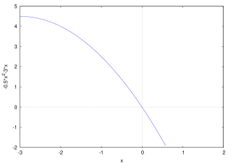
(b) $\Pi^{d}(\varsigma)=-0.5\varsigma^{2}-3\varsigma$.

Figure 3: Example 1

4.2 Example 2: The case when $0<|f|^{2}<8{\alpha}^{2}{\lambda}^{3}/27$

Consider $n=2$, ${\alpha}=1$, ${\lambda}=3$ and $f=(1,1)$. In this case, the functions $\Pi$ and $\Pi^{d}$ are given in figure 5.

Using Equations (8)-(10), it is not hard to show that the three stationary points of $\Pi^{d}$ are $\varsigma_{1}=2\cdot\cos 40^{\circ}-1,\ \varsigma_{2}=2\cdot\cos 80^{\circ}-1$ and $\varsigma_{3}=2\cdot\cos 160^{\circ}-1$.

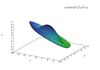
(a) $\Pi(x,y)=0.5(0.5(x^{2}+y^{2})-3)^{2}-x-y$.

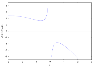
(b) $\Pi^{d}(\varsigma)=(-1/\varsigma)-0.5\varsigma^{2}-3\varsigma$.

Figure 4: Example 2

Let us highlight that in this case, $t=0$ could be a minimizer or a maximizer of the function $\phi(t)=\Pi(x_{2}+tz)$, where $x_{2}=f/\varsigma_{2}$ and $z\in{I\!\!R}^{n}$ is an arbitrary chosen vector. If we consider $z=(1,-1)$ we have that the graph of $\phi$ is given by figure 5a and if we consider $z=(0.2,1.4)$ we have that the graph of $\phi$ is given by figure 5b.

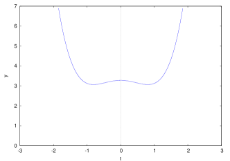
(a) Function $\phi$ with $z=(1,-1)$.

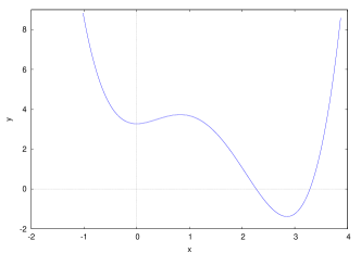
(b) Function $\phi$ with $z=(0.2,1.4)$.

Figure 5: Function $\phi$

Clearly, $t=0$ is a local maximizer for $\phi$ if $z=(1,-1)$ and a local minimizer if $z=(0.2,1.4)$.

4.3 Example 3: The case when $|f|^{2}=8{\alpha}^{2}{\lambda}^{3}/27$

Consider $n=2$, ${\alpha}=1$, ${\lambda}=3$ and $f=(2,2)$. In this case, the functions $\Pi$ and $\Pi^{d}$ are given in figure 6.

(a) $\Pi(x,y)=0.5(0.5(x^{2}+y^{2})-3)^{2}-2x-2y$.

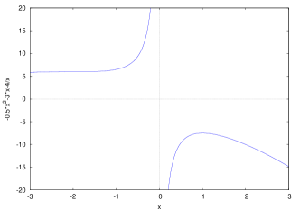
(b) $\Pi^{d}(\varsigma)=(-4/\varsigma)-0.5\varsigma^{2}-3\varsigma$.

Figure 6: Example 3

Using Equations (8)-(10), it is not hard to show that the three stationary points of $\Pi^{d}$ are $\varsigma_{1}={\lambda}/3,\ \varsigma_{2}=\varsigma_{3}=-2{\lambda}/3$.

4.4 Example 4: The case when $8{\alpha}^{2}{\lambda}^{3}/27<|f|^{2}$

Consider $n=2$, ${\alpha}=1$, ${\lambda}=3$ and $f=(3,3)$. In this case, the functions $\Pi$ and $\Pi^{d}$ are given in figure 7.

(a) $\Pi(x,y)=0.5(0.5(x^{2}+y^{2})-3)^{2}-3x-3y$.

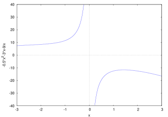
(b) $\Pi^{d}(\varsigma)=(-9/\varsigma)-0.5\varsigma^{2}-3\varsigma$.

Figure 7: Example 4

From Equations (5)-(7), it is not hard to show that the only real stationary point of $\Pi^{d}$ is $\varsigma_{1}$.

5 Concluding Remarks

A complete set of analytical solutions is presented in this paper for a nonconvex optimization problem with double-well potential in ${I\!\!R}^{n}$. The open problem on the double-min duality left in 2003 has been solved for this special case. But the method and idea developed in this paper pave the way to prove the triality theory in general global optimization problems [11, 13, 15]. The perturbation Theorem 3 shows that if the primal problem has more than one global minimizer, the linear canonical dual perturbation method and the triality theory can be used for finding both global minimizer and local extrema. It was first realized in [6] that the primal problem could be NP-hard if it has more than one global minimizer. Therefore, this linear perturbation method should play a key role in solving some challenging problems in global optimization (see [18]). Nonlinear perturbation method for solving NP-hard integer programming problems has been discussed in [9].

References

[1]
Arnold, V. I.
Mathematical Methods of Classical Mechanics.Springer-Verlag Berlin Heidelberg (1989, 2nd Edition).
[2]
Desoer, C. A.; Whalen, B. H.
A Note on Pseudoinverses.Journal of the Society for Industrial and Applied
Mathematics, Vol. 11, No 2, pp. 442-447 (1963).
[3]
Gao, D. Y.
Duality Principles in nonconvex systems. Theory
Methods and Applications.Kluwer Academic Publishers, Dordrecht/Boston/London
(2000).
[4]
Gao, D. Y.
Perfect duality theory and complete solutions to a class of global optimization problems.Optim. 52(4–5), 467–493(2003).
[5]
Gao, D. Y.
Nonconvex semi-linear problems and canonical duality solutions.,
Advances in Mechanics and Mathematics, D.Y. Gao and R.W. Ogden (eds). Kluwer, 261-311 (2003)
[6]
Gao, D. Y.
Solutions and optimality to box constrained nonconvex minimization problems.J. Ind. Manag. Optim. 3(2), 293–304, (2007).
[7]
Gao, D. Y.