Add-ons for Lattice Boltzmann Methods: Regularization, Filtering and Limiters

R.A. Brownlee, J. Levesley, D. Packwood and A.N. Gorban

Department of Mathematics, University of Leicester, Leicester LE1 7RH, UK

Abstract: We describe how regularization of lattice Boltzmann methods can be achieved by modifying dissipation. Classes of techniques used to try to improve regularization of LBMs include flux limiters, enforcing the exact correct production of entropy and manipulating non-hydrodynamic modes of the system in relaxation. Each of these techniques corresponds to an additional modification of dissipation compared with the standard LBGK model. Using some standard 1D and 2D benchmarks including the shock tube and lid driven cavity, we explore the effectiveness of these classes of methods.

Keywords: Lattice Boltzmann, Dissipation, Stability, Entropy, Filtering, Multiple Relaxation Times (MRT), Shock Tube, Lid-Driven Cavity

1. INTRODUCTION

Lattice Boltzmann methods (LBM) are a class of discrete computational schemes which can be used to simulate hydrodynamics and more[33]. They have been proposed as a discretization of Boltzmann’s kinetic equation. Instead of fields of moments $M$, the LBM operates with fields of discrete distributions $f$.

All computational methods for continuum dynamics meet some troubles with stability when the gradients of the flows become too sharp. In Computational Fluid Dynamics (CFD) such situations occur when the Mach number $Ma$ is not small, or the Reynolds number $Re$ is too large. The possibility for using grid refinement is bounded by computational time and memory restrictions. Moreover, for nonlinear systems with shocks then grid refinement does not guarantee convergence to the proper solution. Methods of choice to remedy this are based on the modification of dissipation with limiters, additional viscosity, and so on [36]. All these approaches combine high order methods in relatively quiet regions with low order regularized methods in the regions with large gradients. The areas of the high-slope flows are assumed to be small but the loss of the order of accuracy in a small region may affect the accuracy in the whole domain because of the phenomenon of error propagation. Nevertheless, this loss of accuracy for systems with high gradients seems to be unavoidable.

It is impossible to successfully struggle with some spurious effects without a local decrease in the order of accuracy. In a more formal setting, this has been proven. In 1959, Godunov [14] proved that a (linear) scheme for a partial differintial equation could not, at the same time, be monotone and second-order accurate. Hence, we should choose between spurious oscillations in high order non-monotone schemes and additional dissipation in first-order schemes. Lax [23] demonstrated that un-physical dispersive oscillations in areas with high slopes are unavoidable due to discretization. For hydrodynamic simulations using the standard LBGK model (Sec. 1) such oscillations become prevalent especially at high $Re$ and non-small $Ma$. Levermore and Liu used differential approximation to produce the “modulation equation" for the dispersive oscillation in the simple initial-value Hopf problem [24] and demonstrated directly how for a nonlinear problem a solution of the discretized equation does not converge to the solution of the continuous model with high slope when the step $h\to 0$.

Some authors expressed a hope that precisely keeping the entropy balance can make the computation more “physical", and that thermodynamics can help to suppress nonphysical effects. Tadmor and Zhong constructed a new family of entropy stable difference schemes which retain the precise entropy decay of the Navier–Stokes equations and demonstrated that this precise keeping of the entropy balance does not help to avoid the nonphysical dispersive oscillations [34].

To prevent nonphysical oscillations, most upwind schemes employ limiters that reduce the spatial accuracy to first order through shock waves. A mixed-order scheme may be defined as a numerical method where the formal order of the truncation error varies either spatially, for example, at a shock wave, or for different terms in the governing equations, for example, third-order convection with second-order diffusion [31].

Several techniques have been proposed to help suppress these pollutive oscillations in LBM, the three which we deal with in this work are entropic lattice Boltzman (ELBM), entropic limiters and generalized lattice Boltzmann, also known as multiple relaxation time lattice Boltzmann (MRT). Where effective each of these techniques corresponds to an additional degree of complexity in the dissipation to the system, above that which exists in the LBGK model.

The Entropic lattice Boltzmann method (ELBM) was invented first in 1998 as a tool for the construction of single relaxation time LBM which respect the $H$-theorem [19]. For this purpose, instead of the mirror image with a local equilibrium as the reflection center, the entropic involution was proposed, which preserves the entropy value. Later, it was called the Karlin-Succi involution [15]. In 2000, it was reported that exact implementation of the Karlin-Succi involution (which keeps the entropy balance) significantly regularizes the post-shock dispersive oscillations [1]. This regularization seems very surprising, because the entropic lattice BGK (ELBGK) model gives a second-order approximation to the Navier–Stokes equation similarly to the LBGK model (different proofs of that degree of approximation were given in [33] and [4]).

Entropic limiters [4] are an example of flux limiter schemes [4, 21, 29], which are invented to combine high resolution schemes in areas with smooth fields and first order schemes in areas with sharp gradients. The idea of flux limiters can be illustrated by the computation of the flux $F_{0,1}$ of the conserved quantity $u$ between a cell marked by 0 and one of two its neighbour cells marked by $\pm 1$:

$$F_{0,1}=(1-\phi(r))f^{\rm low}_{0,1}+\phi(r)f^{\rm high}_{0,1},$$ (1)

where $f^{\rm low}_{0,\,1}$, $f^{\rm high}_{0,\,1}$ are low and high resolution scheme fluxes, respectively, $r=(u_{0}-u_{-1})/(u_{1}-u_{0})$, and $\phi(r)\geq 0$ is a flux limiter function. For $r$ close to 1, the flux limiter function $\phi(r)$ should be also close to 1. Many flux limiter schemes have been invented during the last two decades [36]. No particular limiter works well for all problems, and a choice is usually made on a trial and error basis. Particular examples of the limiters we use are introduced in Section 3.3..

MRT has been developed as a true generalization of the collisions in the lattice Bhatnagar–Gross–Krook (LBGK) scheme [11, 22] from a one parameter diagonal relaxation matrix, to a general linear operation with more free parameters, the number of which is dependent on the particular discrete velocity set used and the number of conserved macroscopic variables. Different variants of MRT have been shown to improve accuracy and stability, including in our benchmark examples [26] in comparison with the standard LBGK systems.

The lattice Boltzmann paradigm is now mature, and explanations for some of its successes are available. However, in its applications it approaches the boundaries of the applicability and need special additional tools to extend the area of applications. It is well-understood that near to shocks, for instance, special and specific attention must be paid to avoid unphysical effects. In this paper then, we will discuss a variety of add-ons for LBM and apply them to a variety of standard 1D and 2D problems to test their effectiveness. In particular we will describe a family of entropic filters and show that we can use them to signficantly expand the effective range of operation of the LBM.

2. BACKGROUND

Lattice Boltzmann methods can be derived independently by a discretization Boltzmann’s equation for kinetic transport or by naively creating a discrete scheme which matches moments with the Maxwellian distribution up to some finite order.

In each case the final discrete algorithm consists of two alternating steps, advection and collision, which are applied to $m$ single particle distribution functions $f_{i}\equiv f_{i}(\mathbf{x},t),(i=1\ldots m)$, each of which corresponds with a discrete velocity vector $\mathbf{v}_{i},(i=1\ldots m)$. The values $f_{i}$ are also sometimes known as populations or densities as they can be thought of as representative of the densities of particles moving in the direction of the corresponding discrete velocities.

The advection operation is simply free flight for the discrete time step $\epsilon$ in the direction of the corresponding velocity vector,

$$f_{i}(\mathbf{x},t+\epsilon)=f_{i}(\mathbf{x}-\epsilon\mathbf{v}_{i},t).$$ (2)

The collision operation is instantaneous and can be different for each distribution function but depends on every distribution function, this might be written,

$$f_{i}(\mathbf{x})\rightarrow F_{i}(\{f_{i}(\mathbf{x})\}).$$ (3)

In order to have a slightly more compact notation we can write these operations in vector form, in the below equation it should be inferred that the $i$th distribution function is advecting along its corresponding discrete velocity,

$$\mathbf{f}(\mathbf{x},t+\epsilon)=\mathbf{f}(\mathbf{x}-\epsilon\mathbf{v}_{i},t),$$ (4)

$$\mathbf{f}(\mathbf{x})\rightarrow F(\mathbf{f}(\mathbf{x})).$$ (5)

To transform our vector of microscopic variables at a point in space $\mathbf{f}(\mathbf{x})$ to a vector of macroscopic variables $M(\mathbf{x})$ we use a vector of linear functions $M(\mathbf{x})=m(\mathbf{f}(\mathbf{x}))$. In the athermal hydrodynamic systems we consider in this work the momemts are density $\rho$ and momentum density $\rho\mathbf{u}$, $\{\rho,\rho\mathbf{u}\}(\mathbf{x})=\sum_{i}\{1,\mathbf{v}_{i}\}f_{i}(\mathbf{x})$. These macroscopic moments are conserved by the collision operation, $m(\mathbf{f})=m(F(\mathbf{f}))$.

The simplest and most common choice for the collision operation $F$ is the Bhatnagar-Gross-Krook(BGK) [7, 9, 17, 33] operator with over-relaxation

$$F(\mathbf{f})=\mathbf{f}+\alpha\beta(\mathbf{f}^{\mathrm{eq}}-\mathbf{f}).$$ (6)

For the standard LBGK method $\alpha=2$ and $\beta\in[0,1]$ (usually, $\beta\in[1/2,1]$) is the over-relaxation coefficient used to control viscosity. For $\beta=1/2$ the collision operator returns the local equilibrium $\mathbf{f}^{\mathrm{eq}}$ and $\beta=1$ (the mirror reflection) returns the collision for a liquid at the zero viscosity limit. The definition of $\mathbf{f}^{\mathrm{eq}}$ defines the dynamics of the system, often it chosen as an approximation to the continuous Maxwellian distribution. An equilibrium can also be independently derived by constructing a discrete system which matches moments of the Maxwellian up to some finite order. For hydrodynamic systems often this finite order is chosen to be 2, as this is sufficient to accurately replicate the Euler(non dissipative) component of the Navier Stokes equations. For a dissipative fluid with viscosity $\nu$ the parameter $\beta$ is chosen by $\beta=\epsilon/(2\nu+\epsilon)$.

Each of the techniques we test in this paper can be introduced as developments of the generic LBGK system and such a presentation follows in the next sections.

3. ENTROPIC LATTICE BOLTZMANN

3.1. LBM with $H$ theorem

In the continuous case the Maxwellian distribution maximizes entropy, as measured by the Boltzmann $H$ function, and therefore also has zero entropy production. In the context of lattice Boltzmann methods a discrete form of the $H$-theorem has been suggested as a way to introduce thermodynamic control to the system [18, 1].

From this perspective the goal is to find an equilibrium state equivalent to the Maxwellian in the continuum which will similarly maximize entropy. Before the equilibrium can be found an appropriate $H$ function must be known for a given lattice. These functions have been constructed in a lattice dependent fashion in [18], and $H=-S$ with $S$ from (7) is an example of a $H$ function constructed in this way.

One way to implement an ELBM is as a variation on the LBGK, known as the ELBGK [1]. In this case $\alpha$ is varied to ensure a constant entropy condition according to the discrete $H$-theorem. In general the entropy function is based upon the lattice and cannot always be found explicitly. However for some examples such as the simple one dimensional lattice with velocities $\mathbf{v}=(-c,0,c)$ and corresponding populations $\mathbf{f}=(f_{-},f_{0},f_{+})$ an explicit Boltzmann style entropy function is known [18]:

$$S(\mathbf{f})=-f_{-}\log(f_{-})-f_{0}\log(f_{0}/4)-f_{+}\log(f_{+}).$$ (7)

With knowledge of such a function $\alpha$ is found as the non-trivial root of the equation

$$S(\mathbf{f})=S(\mathbf{f}+\alpha(\mathbf{f}^{\ast}-\mathbf{f})).$$ (8)

The trivial root $\alpha=0$ returns the entropy value of the original populations. ELBGK then finds the non-trivial $\alpha$ such that (8) holds. This version of the BGK collision one calls entropic BGK (or EBGK) collision. A solution of (8) must be found at every time step and lattice site. Entropic equilibria (also derived from the $H$-theorem) are always used for ELBGK.

3.2. ELBM algorithm and additional dissipation

The definition of ELBM for a given entropy equation (8) is incomplete. First of all, it is possible that the non-trivial solution does not exist. Moreover, for most of the known entropies (like the perfect entropy [18]) there always exist such $f$ that the equation (8) for the ELBM collision has no non-trivial solutions. These $f$ should be sufficiently far from equilibrium. For completeness, every user of ELBM should define collisions when the non-trivial root of (8) does not exist. We know and tried two rules for this situation:

1. The most radical approach gives the the Ehrenfest rule [16, 3]: ”if the solution does not exist then go to equilibrium", i.e. if the solution does not exists then take $\alpha=1$.

2. The most gentle solution gives the ”positivity rule" [3, 25, 35, 32]: to take the maximal value of $\alpha$ that guarantees $f_{i}+\alpha(f_{i}^{\ast}-f_{i})\geq 0$ for all $i$.

In general, the Ehrenfest rule prescribes to send the most non-equilibrium sites to equilibrium and the positivity rule is applied for any LBM as a recommendation to substitute the non-positive vectors $\mathbf{f}$ by the closest non-negative on the interval of the straight line $[\mathbf{f},\mathbf{f}^{\ast}]$ that connects $\mathbf{f}$ to equilibrium. These rules give the examples of the pointwise LBM limiter and we discuss them separately.

By its nature, the ELBM adds more dissipation than the positivity rule when the non-trivial root of (8) does not exist. It does not always keep the entropy balance but increases dissipation for highly nonequilibrium sites.

3.3. Numerical method for solution of the ELBM equation

Another source for additional dissipation in the ELBM may be the numerical method used for the solution of (8). For the full description of ELBM we have to select a numerical method for this equation. This method has to have an uniform accuracy in the wide range of parameters, for all possible deviation from equilibrium (distribution of these deviations has “heavy tails" [5]).

In order to investigate the stabilization properties of ELBGK it is necessary to craft a numerical method capable of finding the non-trivial root in (8). In this section we fix the population vectors $\mathbf{f}$ and $\mathbf{f}^{*}$, and are concerned only with this root finding algorithm. We recast (8) as a function of $\alpha$ only:

$$S_{f}(\alpha)=S(\mathbf{f}+\alpha(\mathbf{f}^{\mathrm{eq}}-\mathbf{f}))-S(\mathbf{f}).$$ (9)

In this setting we attempt to find the non-trivial root $r$ of (9) such that $S_{f}(r)=0$. It should be noted that as we search for $r$ numerically we should always take care that the approximation we use is less than $r$ itself. An upper approximation could result in negative entropy production. A simple algorithm for finding the roots of a concave function, based on local quadratic approximations to the target function, has cubic convergence order. Assume that we are operating in a neighbourhood $r\in N$, in which $S_{f}^{\prime}$ is negative (as well of course $S_{f}^{\prime\prime}$ is negative). At each iteration the new estimate for $r$ is the greater root of the parabola $P$, the second order Taylor polynomial at the current estimate. Analogously to the case for Newton iteration, the constant in the estimate is the ratio of third and first derivatives in the interval of iteration:

$$|(r-\alpha_{n+1})|\,\leq\,C|\alpha_{n}-r|^{3},$$

$$\mbox{where}\;\;C=\frac{1}{6}\sup_{a\in N}|S_{f}^{\prime\prime\prime}(a)|\left/\inf_{b\in N}|S_{f}^{\prime}(b)|\right.,$$

where $\alpha_{n}$ is the evaluation of $r$ on the $n$th iteration.

We use a Newton step to estimate the accuracy of the method at each iteration: because of the concavity of $S$

$$|\alpha_{n}-r|\lesssim\left|S_{f}(\alpha_{n})/S_{f}^{\prime}(\alpha_{n})\right|.$$ (10)

In fact we use a convergence criteria based not solely on $\alpha$ but on $\alpha||\mathbf{f}^{*}-\mathbf{f}||$, this has the intuitive appeal that in the case where the populations are close to the local equilibrium $\Delta S=S(\mathbf{f}^{*})-S(\mathbf{f})$ will be small and a very precise estimate of $\alpha$ is unnecessary. We have some freedom in the choice of the norm used and we select between the standard $L_{1}$ norm and the entropic norm. The entropic norm is defined as

$$||\mathbf{f}^{\mathrm{eq}}-\mathbf{f}||_{\mathbf{f}^{\mathrm{eq}}}=-((\mathbf{f}^{\mathrm{eq}}-\mathbf{f}),\left.D^{2}S\right|_{\mathbf{f}^{\mathrm{eq}}}(\mathbf{f}^{\mathrm{eq}}-\mathbf{f})),$$

where $\left.D^{2}S\right|_{\mathbf{f}^{\mathrm{eq}}}$ is the second differential of entropy at point $\mathbf{f}^{\mathrm{eq}}$, and $(x,y)$ is the standard scalar product.

The final root finding algorithm then is beginning with the LBGK estimate $x_{0}=2$ to iterate using the roots of successive parabolas. We stop the method at the point,

$$|\alpha_{n}-r|\cdot||\mathbf{f}^{*}-\mathbf{f}||<\epsilon.$$ (11)

To ensure that we use an estimate that is less than the root, at the point where the method has converged we check the sign of $S_{f}(\alpha_{n})$. If $S_{f}(\alpha_{n})>0$ then we have achieved a lower estimate, if $S_{f}(\alpha_{n})<0$ we correct the estimate to the other side of the root with a double length Newton step,

$$\alpha_{n}=\alpha_{n}-2\frac{S_{f}(\alpha_{n})}{S_{f}^{\prime}(\alpha_{n})}.$$ (12)

At each time step before we begin root finding we eliminate all sites with $\Delta S<10^{-15}$. For these sites we make a simple LBGK step. At such sites we find that round off error in the calculation of $S_{f}$ by solution of equation (8) can result in the root of the parabola becoming imaginary. In such cases a mirror image given by LBGK is effectively indistinct from the exact ELBGK collision. In the numerical examples given in this work the case where the non-trivial root of the entropy parabola does not exist was not encountered.

4. ENTROPIC FILTERING

All the specific LBM limiters [5, 29] are based on a representation of distributions $f$ in the form:

$$\mathbf{f}=\mathbf{f}^{\mathrm{eq}}+\|\mathbf{f}-\mathbf{f}^{\mathrm{eq}}\|\frac{\mathbf{f}-\mathbf{f}^{\mathrm{eq}}}{\|\mathbf{f}-\mathbf{f}^{\mathrm{eq}}\|},$$ (13)

where $\mathbf{f}^{\mathrm{eq}}$ is the corresponding quasiequilibrium (conditional equilibrium) for given moments $M$, $\mathbf{f}-\mathbf{f}^{\mathrm{eq}}$ is the nonequilibrium “part" of the distribution, which is represented in the form “norm$\times$direction” and $\|f-f^{*}\|$ is the norm of that nonequilibrium component (usually this is the entropic norm).

All limiters we use change the norm of the nonequilibrium component $\mathbf{f}-\mathbf{f}^{\mathrm{eq}}$, but do not touch its direction or the quasiequilibrium. In particular, limiters do not change the macroscopic variables, because moments for $\mathbf{f}$ and $\mathbf{f}^{\mathrm{eq}}$ coincide. These limiters are transformations of the form

$$\mathbf{f}\mapsto\mathbf{f}^{\mathrm{eq}}+\phi\times(\mathbf{f}-\mathbf{f}^{\mathrm{eq}})$$ (14)

with $\phi>0$. If $\mathbf{f}-\mathbf{f}^{\mathrm{eq}}$ is too big, then the limiter should decrease its norm.

For the first example of the realization of this pointwise filtering we use the kinetic idea of the positivity rule, the prescription is simple [3, 25, 35, 32]: to substitute nonpositive $F(\mathbf{f})$ by the closest nonnegative state that belongs to the straight line

$$\Bigr{\{}\lambda\mathbf{f}+(1-\lambda)\mathbf{f}^{\mathrm{eq}}|\>\lambda\in\mathbb{R}\Bigl{\}}$$ (15)

defined by the two points, $\mathbf{f}$ and the corresponding quasiequilibrium (1). This operation is to be applied pointwise, at points of the lattice where positivity is violated. This technique preserves the positivity of populations, but can affect the accuracy of the approximation. This rule is necessary for ELBM when the positive “mirror state” with the same entropy as $\mathbf{f}$ does not exists on the straight line (15).

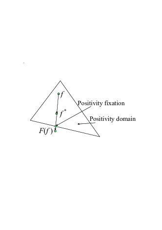
Fig. (1): Positivity rule in action. The motions stops at the positivity boundary.

The positivity rule measures the deviation $f-f^{*}$ by a binary measure: if all components of this vector $f-f^{*}$ are non-negative then it is not too large. If some of them are negative that this deviation is too large and needs corrections.

To construct pointwise flux limiters for LBM, based on dissipation, the entropic approach remains very convenient. The local nonequilibrium entropy for each site is defined

$$\Delta S(\mathbf{f}):=S(\mathbf{f}^{\mathrm{eq}})-S(\mathbf{f}).$$ (16)

The positivity limiter was targeted wherever population densities became negative. Entropic limiters are targeted wherever non-equilibrium entropy becomes large.

The first limiter is Ehrenfests’ regularisation [4, 3], it provides “entropy trimming”: we monitor local deviation of $\mathbf{f}$ from the corresponding quasiequilibrium, and when $\Delta S(\mathbf{f})(\mathbf{x})$ exceeds a pre-specified threshold value $\delta$, perform local Ehrenfests’ steps to the corresponding equilibrium: $\mathbf{f}\mapsto\mathbf{f}^{\mathrm{eq}}$ at those points.

Not all lattice Boltzmann models are entropic, and an important question arises: “how can we create nonequilibrium entropy limiters for LBM with non-entropic (quasi)equilibria?”. We propose a solution of this problem based on the discrete Kullback entropy [20]:

$$S_{\rm K}(\mathbf{f})=-\sum_{i}f_{i}\ln\biggl{(}\frac{f_{i}}{f_{i}^{\rm eq}}\biggr{)}.$$ (17)

For entropic quasiequilibria with perfect entropy the discrete Kullback entropy gives the same $\Delta S$: $-S_{\rm K}(f)=\Delta S(f)$. Let the discrete entropy have the standard form for an ideal (perfect) mixture [18]:

$$S(\mathbf{f})=-\sum_{i}f_{i}\ln\biggl{(}\frac{f_{i}}{W_{i}}\biggr{)}.$$

In quadratic approximation,

$$-S_{\rm K}(\mathbf{f})=\sum_{i}f_{i}\ln\biggl{(}\frac{f_{i}}{f^{\rm eq}_{i}}\biggr{)}\approx\sum_{i}\frac{(f_{i}-f^{\rm eq}_{i})^{2}}{f^{\rm eq}_{i}}.$$ (18)

If we define $\mathbf{f}$ as the conditional entropy maximum for given $M_{j}=\sum_{k}m_{jk}f_{k}$, then

$$\ln f^{\rm eq}_{k}=\sum_{j}\mu_{j}m_{jk},$$

where $\mu_{j}(M)$ are the Lagrange multipliers (or “potentials”). For this entropy and conditional equilibrium we find

$$\Delta S=S(\mathbf{f}^{\mathrm{eq}})-S(\mathbf{f})=\sum_{i}f_{i}\ln\biggl{(}\frac{f_{i}}{f^{\rm eq}_{i}}\biggr{)}=-S_{\rm K}(\mathbf{f}),$$ (19)

if $\mathbf{f}$ and $\mathbf{f}^{\mathrm{eq}}$ have the same moments, $m(\mathbf{f})=m(\mathbf{f}^{\mathrm{eq}})$.

In what follows, $\Delta S$ is the Kullback distance $-S_{\rm K}(\mathbf{f}^{\mathrm{eq}})$ (19) for general (positive) quasiequilibria $\mathbf{f}^{\mathrm{eq}}$, or simply $S(\mathbf{f}^{\mathrm{eq}})-S(\mathbf{f})$ for entropic quasiequilibria (or second approximations for these quantities (18)).

So that the Ehrenfests’ steps are not allowed to degrade the accuracy of LBGK it is pertinent to select the $k$ sites with highest $\Delta S>\delta$. An a posteriori estimate of added dissipation could easily be performed by the analysis of entropy production in the Ehrenfests’ steps. Numerical experiments show (see, e.g., [4, 3]) that even a small number of such steps drastically improves stability.

The positivity rule and Ehrenfests’ regularisation provide rare, intense and localised corrections. Of course, it is easy and also computationally cheap to organise more gentle transformations with a smooth shift of highly nonequilibrium states to quasiequilibrium. The following regularisation transformation with a smooths function $\phi$ distributes its action smoothly:

$$\mathbf{f}\mapsto\mathbf{f}^{\mathrm{eq}}+\phi(\Delta S(\mathbf{f}))(\mathbf{f}-\mathbf{f}^{\mathrm{eq}}).$$ (20)

The choice of function $\phi$ is highly ambiguous, for example, $\phi=1/(1+\alpha\Delta S^{k})$ for some $\alpha>0$ and $k>0$. There are two significantly different choices: (i) ensemble-independent $\phi$ (i.e., the value of $\phi$ depends on local value of $\Delta S$ only) and (ii) ensemble-dependent $\phi$, for example

$$\phi(\Delta S)=\frac{1+(\Delta S/(\alpha{\rm E}(\Delta S)))^{k-1/2}}{1+(\Delta S/(\alpha{\rm E}(\Delta S)))^{k}},$$ (21)

where ${\rm E}(\Delta S)$ is the average value of $\Delta S$ in the computational area, $k\geq 1$, and $\alpha\gtrsim 1$. For small $\Delta S$, $\phi(\Delta S)\approx 1$ and for $\Delta S\gg\alpha{\rm E}(\Delta S)$ it tends to $\sqrt{\alpha{\rm E}(\Delta S)/\Delta S}$. It is easy to select an ensemble-dependent $\phi$ with control of total additional dissipation.

4.1. Monotonic and double monotonic limiters

Two monotonicity properties are important in the theory of nonequilibrium entropy limiters:

1. A limiter should move the distribution to equilibrium: in all cases of (14) $0\leq\phi\leq 1$. This is the dissipativity condition which means that limiters never produce negative entropy.

2. A limiter should not change the order of states on the line: if for two distributions with the same moments, $\mathbf{f}$ and $\mathbf{f}^{\prime}$, $\mathbf{f}^{\prime}-\mathbf{f}^{\mathrm{eq}}=x(\mathbf{f}-\mathbf{f}^{\mathrm{eq}})$ and $\Delta S(\mathbf{f})>\Delta S(\mathbf{f}^{\prime})$ before the limiter transformation, then the same inequality should hold after the limiter transformation too. For example, for the limiter (20) it means that $\Delta S(\mathbf{f}^{\mathrm{eq}}+x\phi(\Delta S(\mathbf{f}^{\mathrm{eq}}+x(\mathbf{f}-\mathbf{f}^{\mathrm{eq}}))(\mathbf{f}-\mathbf{f}^{\mathrm{eq}}))$ is a monotonically increasing function of $x>0$.

In quadratic approximation,

$$\Delta S(\mathbf{f}^{\mathrm{eq}}+x(\mathbf{f}-\mathbf{f}^{\mathrm{eq}})) =x^{2}\Delta S(\mathbf{f}),$$

$$\Delta S(\mathbf{f}^{\mathrm{eq}}+x\phi(\Delta S(\mathbf{f}^{\mathrm{eq}}+x(\mathbf{f}-\mathbf{f}^{\mathrm{eq}}))(\mathbf{f}-\mathbf{f}^{\mathrm{eq}})) =x^{2}\phi^{2}(x^{2}\Delta S(\mathbf{f})),$$

and the second monotonicity condition transforms into the following requirement: $y\phi(y^{2}s)$ is a monotonically increasing (not decreasing) function of $y>0$ for any $s>0$.

If a limiter satisfies both monotonicity conditions, we call it “double monotonic”. For example, Ehrenfests’ regularisation satisfies the first monotonicity condition, but violates the second one. The limiter (21) violates the first condition for small $\Delta S$, but is dissipative and satisfies the second one in quadratic approximation for large $\Delta S$. The limiter with $\phi=1/(1+\alpha\Delta S^{k})$ always satisfies the first monotonicity condition, violates the second if $k>1/2$, and is double monotonic (in quadratic approximation for the second condition), if $0<k\leq 1/2$. The threshold limiter (26) is also double monotonic.

For smooth functions, the condition of double monotonicity (in quadratic approximation) is equivalent to the system of differential inequalities:

$$\begin{split}\phi(x)+2x\phi^{\prime}(x)&\geq 0;\\ \phi^{\prime}(x)&\leq 0.\end{split}$$

The initial condition $\phi(0)=1$ means that in the limit $\Delta S\to 0$ limiters do not affect the flow. Following these inequalities we can write: $2x\phi^{\prime}(x)=-\eta(x)\phi(x)$, where $0\leq\eta(x)\leq 1$. The solution of these inequalities with initial condition is

$$\phi(x)=\exp\biggl{(}-\frac{1}{2}\int_{0}^{x}\frac{\eta(\chi)}{\chi}{\mathrm{d}}\chi\biggr{)},$$ (22)

if the integral on the right-hand side exists. This is a general solution for double monotonic limiters (in the second approximation for entropy). If $\eta(x)$ is the Heaviside step function, $\eta(x)=H(x-\Delta S_{\rm t})$ with threshold value $\Delta S_{\rm t}$, then the general solution (22) gives us the threshold limiter. If, for example, $\eta(x)=x^{k}/(\Delta S_{\rm t}^{k}+x^{k})$, then

$$\phi(x)=\left(1+\frac{x^{k}}{\Delta S_{\rm t}^{k}}\right)^{-\frac{1}{2k}}.$$ (23)

This special form of limiter function is attractive because for small $x$ it gives

$$\phi(x)=1-\frac{1}{2k}\frac{x^{k}}{\Delta S_{\rm t}^{k}}+o(x^{k}).$$

Thus, the limiter does not affect the motion up to the $(k+1)$st order, and the macroscopic equations coincide with the macroscopic equations for LBM without limiters up to the $(k+1)$st order in powers of deviation from quasiequilibrium. Furthermore, for large $x$ we get the $k$th order approximation to the threshold limiter (26):

$$\phi(x)=\sqrt{\frac{\Delta S_{\rm t}}{x}}+o(x^{-k}).$$

Of course, it is not forbidden to use any type of limiters under the local and global control of dissipation, but double monotonic limiters provide some natural properties automatically, without additional care.

4.2. Monitoring total dissipation

For given $\beta$, the entropy production in one LBGK step in quadratic approximation for $\Delta S$ is:

$$\delta_{\rm LBGK}S\approx[1-(2\beta-1)^{2}]\sum_{x}\Delta S(\mathbf{x}),$$

where $\mathbf{x}$ is the grid point, $\Delta S(\mathbf{x})$ is nonequilibrium entropy (16) at point $\mathbf{x}$, $\delta_{\rm LBGK}S$ is the total entropy production in a single LBGK step. It would be desirable if the total entropy production for the limiter $\delta_{\rm lim}S$ was small relative to $\delta_{\rm LBGK}S$:

$$\delta_{\rm lim}S<\delta_{0}\delta_{\rm LBGK}S.$$ (24)

A simple ensemble-dependent limiter (perhaps, the simplest one) for a given $\delta_{0}$ operates as follows. Let us collect the histogram of the $\Delta S(\mathbf{x})$ distribution, and estimate the distribution density, $p(\Delta S)$. We have to estimate a value $\Delta S_{0}$ that satisfies the following equation:

$$\int_{\Delta S_{0}}^{\infty}p(\Delta S)(\Delta S-\Delta S_{0})\,{\mathrm{d}}\Delta S=\delta_{0}[1-(2\beta-1)^{2}]\int_{0}^{\infty}p(\Delta S)\Delta S\,{\mathrm{d}}\Delta S.$$ (25)

In order not to affect distributions with a small expectation of $\Delta S$, we choose a threshold $\Delta S_{\rm t}=\max\{\Delta S_{0},\delta\}$, where $\delta$ is some predefined value (as in the Ehrenfests’ regularization). For states at sites with $\Delta S\geq\Delta S_{\rm t}$ we provide homothety with equilibrium center $\mathbf{f}^{\mathrm{eq}}$ and coefficient $\sqrt{\Delta S_{\rm t}/\Delta S}$ (in quadratic approximation for nonequilibrium entropy):

$$\mathbf{f}(\mathbf{x})\mapsto\mathbf{f}^{\mathrm{eq}}(\mathbf{x})+\sqrt{\frac{\Delta S_{\rm t}}{\Delta S}}(\mathbf{f}(\mathbf{x})-\mathbf{f}^{\mathrm{eq}}(\mathbf{x})).$$ (26)

To avoid the change of accuracy order “on average”, the number of sites with this step should be $\leq\mathcal{O}(Nh/L)$ where $N$ is the total number of sites, $h$ is the step of the space discretization and $L$ is the macroscopic characteristic length. But this rough estimate of accuracy across the system might be destroyed by a concentration of Ehrenfests’ steps in the most nonequilibrium areas, for example, in boundary layers. In that case, instead of the total number of sites $N$ in $\mathcal{O}(Nh/L)$ we should take the number of sites in a specific region. The effects of such concentration could be analysed a posteriori.

4.3. Median entropy filter

The Ehrenfest step described above provides pointwise correction of nonequilibrium entropy at the “most nonequilibrium” points. Due to the pointwise nature, the technique does not introduce any nonisotropic effects, and provides some other benefits. But if we involve local structure, we can correct local non-monotone irregularities without touching regular fragments. For example, we can discuss monotone increase or decrease of nonequilibrium entropy as regular fragments and concentrate our efforts on reduction of “speckle noise” or “salt and pepper noise”. This approach allows us to use the accessible resource of entropy change (24) more thriftily. Salt and pepper noise is a form of noise typically observed in images. It represents itself as randomly occurring white (maximal brightness) and black pixels. For this kind of noise, conventional low-pass filtering, e.g., mean filtering or Gaussian smoothing is unsuccessful because the perturbed pixel value can vary significantly both from the original and mean value. For this type of noise, median filtering is a common and effective noise reduction method. Median filtering is a common step in image processing [30] for the smoothing of signals and the suppression of impulse noise with preservation of edges.

The median is a more robust average than the mean (or the weighted mean) and so a single very unrepresentative value in a neighbourhood will not affect the median value significantly. Hence, we suppose that the median entropy filter will work better than entropy convolution filters.

For the nonequilibrium entropy field, the median filter considers each site in turn and looks at its nearby neighbours. It replaces the nonequilibrium entropy value $\Delta S$ at the point with the median of those values $\Delta S_{\rm med}$, then updates $f$ by the transformation (26) with the homothety coefficient $\sqrt{\Delta S_{\rm med}/{\Delta S}}$. The median, $\Delta S_{\rm med}$, is calculated by first sorting all the values from the surrounding neighbourhood into numerical order and then replacing that being considered with the middle value. For example, if a point has 3 nearest neighbours including itself, then after sorting we have 3 values $\Delta S$: $\Delta S_{1}\leq\Delta S_{2}\leq\Delta S_{3}$. The median value is $\Delta S_{\rm med}=\Delta S_{2}$. For 9 nearest neighbours (including itself) we have after sorting $\Delta S_{\rm med}=\Delta S_{5}$. For 27 nearest neighbours $\Delta S_{\rm med}=\Delta S_{14}$.

We accept only dissipative corrections (those resulting in a decrease of $\Delta S$, $\Delta S_{\rm med}<\Delta S$) because of the second law of thermodynamics. The analogue of (25) is also useful for the acceptance of the most significant corrections. In “salt and pepper" terms, we correct the salt (where $\Delta S$ exceeds the median value) and do not touch the pepper.

4.4. General nonlocal filters

The separation of $\mathbf{f}$ in equilibrium and nonequilibrium parts (13) allows one to use any nonlocal filtering procedure. Let $\mathbf{f}^{\rm neq}=\mathbf{f}-\mathbf{f}^{\mathrm{eq}}$. The values of moments for $\mathbf{f}$ and $\mathbf{f}^{\mathrm{eq}}$ coincide, hence we can apply any transformation of the form

$$\mathbf{f}^{\rm neq}(\mathbf{x})\mapsto\sum_{y}d(\mathbf{y})\mathbf{f}^{\rm neq}(\mathbf{x}+\mathbf{y})$$

for any family of vectors $\mathbf{y}$ that shift the grid into itself and any coefficients $d(\mathbf{y})$. If we apply this transformation, the macroscopic variables do not change but their time derivatives may change. We can control the values of some higher moments in order not to perturb significantly some macroscopic parameters, the shear viscosity, for example [10]. Several local (but not pointwise) filters of this type have been proposed and tested recently [29].

5. MULTIPLE RELAXATION TIMES

The MRT lattice Boltzmann system [22, 26, 11] generalizes the BGK collision into a more general linear transformation of the population functions,

$$F(\mathbf{f})=\mathbf{f}+A(\mathbf{f}^{\mathrm{eq}}-\mathbf{f}),$$ (27)

where $A$ is a square matrix of size $m$. The use of this more general operator allows more different parameters to be used within the collision, to manipulate different physical properties, or for stability purposes.

To facilitate this a change of basis matrix can be used to switch the space of the collision to the moment space. Since the moment space of the system may be several dimensions smaller than the population space, to complete the basis linear combinations of higher order polynomials of the discrete velocity vectors may be used. For our later experiments we will use the D2Q9 system, we should select a particular enumeration of the discrete velocity vectors for the system, the zero velocity is numbered one and the positive x velocity is numbered 2, the remainder are numbered clockwise from this system,

$$\begin{array}[]{ccc}7&8&9\\ 6&1&2\\ 5&4&3\end{array}.$$ (28)

The change of basis matrix given in some of the literature [22] is chosen to represent specific macroscopic quantities and in our velocity system is as follows,

$$M_{1}=\left(\begin{array}[]{c c c c c c c c c}1&1&1&1&1&1&1&1&1\\ -4&-1&2&-1&2&-1&2&-1&2\\ 4&-2&1&-2&1&-2&1&-2&1\\ 0&1&1&0&-1&-1&-1&0&1\\ 0&-2&1&0&-1&2&-1&0&1\\ 0&0&-1&-1&-1&0&1&1&1\\ 0&0&-1&2&-1&0&1&-2&1\\ 0&1&0&-1&0&1&0&-1&0\\ 0&0&-1&0&1&0&-1&0&1\end{array}\right)$$ (29)

As an alternative we could complete the basis simply using higher powers of the velocity vectors, the basis would be $1,v_{x},v_{y},v_{x}^{2}+v_{y}^{2},v_{x}^{2}-v_{y}^{2},v_{x}v_{y},v_{x}^{2}v_{y},v_{x}v_{y}^{2},v_{x}^{2}v_{y}^{2}$, in our velocity system then this change of basis matrix is as follows,

$$M_{2}=\left(\begin{array}[]{c c c c c c c c c}1&1&1&1&1&1&1&1&1\\ 0&1&0&-1&0&1&-1&-1&1\\ 0&0&1&0&-1&1&1&-1&-1\\ 0&1&1&1&1&2&2&2&2\\ 0&1&-1&1&-1&0&0&0&0\\ 0&0&0&0&0&1&-1&1&-1\\ 0&0&0&0&0&1&-1&-1&1\\ 0&0&0&0&0&1&1&-1&-1\\ 0&0&0&0&0&1&1&1&1\end{array}\right)$$ (30)

When utilized properly any basis should be equivalent (although with different rates). In any case in this system there are 3 conserved moments and 9 population functions. Altogether then there are 6 degrees of freedom in relaxation in this system. We need some of these degrees of freedom to implement hydrodynamic rates such as shear viscosity or to force isotropy and some are ‘spare’ and can be manipulated to improve accuracy or stability. Typically these spare relaxation modes are sent closer to equilibrium than the standard BGK relaxation rate. This is in effect an additional contraction in the finite dimensional non-equilibrium population function space, corresponding to an increase in dissipation.

Once in moment space we can apply a diagonal relaxation matrix $C_{1}$ to the populations and then the inverse moment transformation matrix $M_{1}^{-1}$ to switch back into population space, altogether $A_{1}=M_{1}^{-1}C_{1}M_{1}$. If we use the standard athermal polynomial equilibria then three entries on the diagonal of $C_{1}$ are actually not important as the moments will be automatically conserved since $m(\mathbf{f})=m(\mathbf{f}^{\mathrm{eq}})$, for simplicity we set them equal to 0 or 1 to reduce the complexity of the terms in the collision matrix. There are 6 more parameters on the diagonal matrix $C$ which we can set. Three of these correspond to second order moments, one each is required for shear and bulk viscosity which are called $s_{e}$ and $s_{\nu}$ respectively and one for isotropy. Two correspond to third order moments, one gives a relaxation rate $s_{q}$ and again one is needed for isotropy. Finally one is used to give a relaxation rate $s_{\epsilon}$ for the single fourth order moment. We have then in total four relaxation parameters which appear on the diagonal matrix in the following form:

$$C_{1}=\left(\begin{array}[]{ c c c c c c c c c}1&0&0&0&0&0&0&0&0\\ 0&s_{e}&0&0&0&0&0&0&0\\ 0&0&s_{\epsilon}&0&0&0&0&0&0\\ 0&0&0&1&0&0&0&0&0\\ 0&0&0&0&s_{q}&0&0&0&0\\ 0&0&0&0&0&1&0&0&0\\ 0&0&0&0&0&0&s_{q}&0&0\\ 0&0&0&0&0&0&0&s_{\nu}&0\\ 0&0&0&0&0&0&0&0&s_{\nu}\end{array}\right).$$ (31)

Apart from the parameter $s_{\nu}$ which is used to control shear viscosity, in an incompressible system the other properties can be varied to improve accuracy and stability. In particular, there exists a variant of MRT known as TRT (two relaxation time) [13] where the relaxation rates $s_{e},s_{\epsilon}$ are made equal to $s_{\nu}$. In a system with boundaries the final rate is calculated $s_{q}=8(2=s_{\nu})/(8-s_{\nu})$, this is done, in particular, to combat numerical slip on the boundaries of the system.

We should say that in some of the literature regarding MRT the equilibrium is actually built in moment space, that is the collision operation would be written,

$$F(\mathbf{f})=\mathbf{f}+M_{1}^{-1}C_{1}(\mathbf{m}^{\mathrm{eq}}-M_{1}\mathbf{f}).$$ (32)

This could be done to increase efficiency, depending on the implementation, however each moment equilibrium $\mathbf{m}^{\mathrm{eq}}$ has an equivalent population space equilibrium $\mathbf{f}^{\mathrm{eq}}=M_{1}^{-1}\mathbf{m}^{\mathrm{eq}}$, so the results of implementing either system should be the same up to rounding error.

We can also conceive of using an MRT type collision as a limiter, that is to apply it only on a small number of points on the lattice where non equilibrium entropy passes a certain threshold. This answers a criticism of the single relaxation time limiters that they fail to preserve dissipation on physical modes. As well as using the standard MRT form given above we can build an MRT limiter using the alternative change of basis matrix $M_{2}$.

The limiter in this case is based on the idea of sending every mode except shear viscosity directly to equilibrium again the complete relaxation matrix is given by $A_{2}=M_{2}^{-1}C_{2}M_{2}$ where,

$$C_{2}=\left(\begin{array}[]{ c c c c c c c c c}1&0&0&0&0&0&0&0&0\\ 0&1&0&0&0&0&0&0&0\\ 0&0&1&0&0&0&0&0&0\\ 0&0&0&1&0&0&0&0&0\\ 0&0&0&0&s_{\nu}&0&0&0&0\\ 0&0&0&0&0&s_{\nu}&0&0&0\\ 0&0&0&0&0&0&1&0&0\\ 0&0&0&0&0&0&0&1&0\\ 0&0&0&0&0&0&0&0&1\end{array}\right).$$ (33)

This could be considered a very aggressive form of the MRT which maximizes regularization on every mode except shear viscosity and would not be appropriate for general use in a system, especially as most systems violate the incompressibility assumption and hence bulk viscosity is not small. The advantage of using the different change of basis matrix is that the complete collision matrix $A_{2}$ is relatively sparse with just twelve off diagonal elements and hence is easy to implement and not too expensive to compute with.

6. 1D SHOCK TUBE

A standard experiment for the testing of LBMs is the one-dimensional shock tube problem. The lattice velocities used are $\mathbf{v}=(-1,0,1)$, so that space shifts of the velocities give lattice sites separated by the unit distance. 800 lattice sites are used and are initialized with the density distribution

$$\rho(x)=\left\{\begin{array}[]{ll}1,&\;\;\;\;1\leq x\leq 400,\\ 0.5,&\;\;\;\;401\leq x\leq 800.\end{array}\right.$$

Initially all velocities are set to zero. We compare the ELBGK equipped with the parabola based root finding algorithm using the entropic norm with the standard LBGK method using both standard polynomial and entropic equilibria. The polynomial equilibria are given in [7, 33]:

$$\begin{split}&f_{-}^{*}=\frac{\rho}{6}\left(1-3u+3u^{2}\right),\;\;f_{0}^{*}=\frac{2\rho}{3}\left(1-\frac{3u^{2}}{2}\right),\\ &f_{+}^{*}=\frac{\rho}{6}\left(1+3u+3u^{2}\right).\end{split}$$

The entropic equilibria also used by the ELBGK are available explicitly as the maximum of the entropy function (7),

$$\begin{split}&f_{-}^{*}=\frac{\rho}{6}(-3u-1+2\sqrt{1\!+\!3u^{2}}),\;\;f_{0}^{*}=\frac{2\rho}{3}(2-\sqrt{1\!+\!3u^{2}}),\\ &f_{+}^{*}=\frac{\rho}{6}(3u-1+2\sqrt{1\!+\!3u^{2}}).\end{split}$$

Now following the prescription fromm Sec. 1 the governing equations for the simulation are

$$\begin{split}&f_{-}(x,t\!+\!1)\!=\!f_{-}(x\!+\!1,t)\!+\!\alpha\beta(f_{-}^{*}(x\!+\!1,t)\!-\!f_{-}(x\!+\!1,t)),\\ &f_{0}(x,t\!+\!1)\!=\!f_{0}(x,t)\!+\!\alpha\beta(f_{0}^{*}(x,t)-f_{0}(x,t)),\\ &f_{+}(x,t\!+\!1)\!=\!f_{+}(x\!-\!1,t)\!+\!\alpha\beta(f_{+}^{*}(x\!-\!1,t)\!-\!f_{+}(x\!-\!1,t)).\end{split}$$

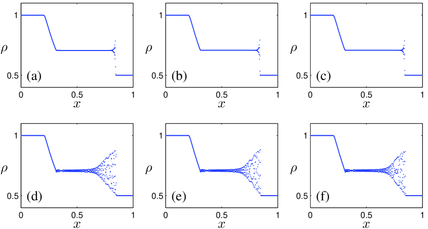
Fig. (2): Density profile of the simulation of the shock tube problem following 400 time steps using (a) LBGK with polynomial equilibria [$\nu=(1/3)\cdot 10^{-1}$]; (b) LBGK with entropic equilibria [$\nu=(1/3)\cdot 10^{-1}$]; (c) ELBGK [$\nu=(1/3)\cdot 10^{-1}$]; (d) LBGK with polynomial equilibria [$\nu=10^{-9}$]; (e) LBGK with entropic equilibria [$\nu=10^{-9}$]; (f) ELBGK [$\nu=10^{-9}$].

From this experiment we observe no benefit in terms of regularization in using the ELBGK rather than the standard LBGK method (Fig. (2)). In both the medium and low viscosity regimes ELBGK does not supress the spurious oscillations found in the standard LBGK method. The observation is in full agreement with the Tadmor and Zhong [34] experiments for schemes with precise entropy balance.

Entropy balance gives a nice additional possibility to monitor the accuracy and the basic physics but does not give an omnipotent tool for regularization.

7. 2D SHEAR DECAY

For the second test we use a simple test proposed to measure the observable viscosity of a lattice Boltzmann simulation to validate the shear viscosity production of the MRT models. We take the 2D isothermal nine-velocity model with standard polynomial equilibria. Our computational domain will a square which we discretize with $L+1\times L+1$ uniformly spaced points and periodic boundary conditions. The initial condition is $\rho(x,y)=1,u_{x}(x,y)=0$ and $u_{y}(x,y)=u_{0}sin(2\pi x/L)$, with $u_{0}=0.05$. The exact velocity solution to this problem is an exponential decay of the initial condition: $u_{x}(x,y,t)=0,u_{y}(x,y,t)=u_{0}\exp(-\lambda u_{0}t/{\rm Re}L)\sin(2\pi x/L)$, where $\lambda$ is some constant and $Re=u_{0}L/\nu$ is the Reynolds number of the flow. Here, $\nu$ is the theoretical shear viscosity of the fluid due to the relaxation parameters of the collision operation.

Now, we simulate the flow over $L/u_{0}$ time steps and measure the constant $\lambda$ from the numerical solution. We do this for LBGK, the ‘aggressive’ MRT with collision matrix $A_{2}$ and the MRT system with collision matrix $A_{1}$ with additional parameters $s_{e}=1.64,s_{\epsilon}=1.54,s_{q}=3(2-s_{\nu})/(3-s_{\nu})$ [22]. The shear viscosity relaxation parameter $s_{\nu}$ is varied to give different viscosities and therefore Reynolds numbers for $L=50$ and for $L=100$.

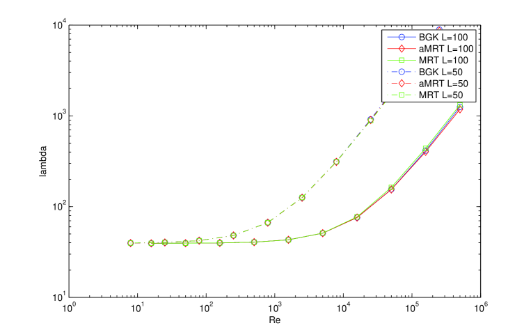
Fig. (3): Observed $\lambda$ in the shear decay experiment

From Figure (3) it can be seen that in all the systems, for increasing theoretical Reynolds numbers (decreasing viscosity coefficient) following a certain point numerical dissipation due to the lattice begins growing. The most important observation from this system is that our MRT models do indeed produce shear viscosity at almost the same rate as the BGK model.

In particular, the bulk viscosity in this system is zero, so all dissipation is given by shear viscosity or higher order modes. Since the space derivatives of the velocity modes are well bounded, as is the magnitude of the velocity itself, the proper asymptotic decay of higher order modes is observed and the varying higher order relaxation coefficients have only a very marginal effect.

We should reiterate that we while we use the ‘aggressive’ MRT across the system, this is only appropriate as bulk viscosity is zero and in fact the selection of the bulk viscosity coefficient makes no difference in this example. This example is a special case in this regard.

8. LID DRIVEN CAVITY

8.1. Stability

Our next 2D example is the benchmark 2D lid driven cavity. In this case this is a square system of side length 129. Bounce back boundary conditions are used and the top boundary imposes a constant velocity of $u_{\rm wall}=0.1$. For a variety of Reynolds numbers we run experiments for up to 10000000 time steps and check which methods have remained stable up until that time step.

The methods which we test are the standard BGK system, the BGK system equipped with Ehrenfest steps, the BGK system equipped with the MRT limiter, the TRT system, an MRT system with the TRT relaxation rate for the third order moment and the other rates $s_{e}=1.64,s_{\epsilon}=1.54$ and finally an MRT system which we call MRT1 with the rates $s_{q}=1.9s_{e}=1.64,s_{\epsilon}=1.54$ [26]. In each case of the system equipped with limiters the maximum number of sites where the limiter is used is 9.

All methods are equipped with the standard 2nd order compressible quasi-equilibrium, which is available as the product of the 1D equilibria 4.4..

When calculating the stream functions of the final states of these simulations we use Simpson integration in first the x and then y directions.

Additionally we measure Enstrophy $\mathcal{E}$ in each system over time. Enstrophy is calculated as the sum of vorticity squared across the system, normalized by the number of lattice sites. This statistic is useful as vorticity is theoretically only dissipated due to shear viscosity, at the same time in the lid driven system vorticity is produced by the moving boundary. For these systems $\mathcal{E}$ becomes constant as the vorticity field becomes steady. The value of this constant indicates where the balance between dissipation and production of vorticity is found. The lower the final value of $\mathcal{E}$ the more dissipation produced in the system.

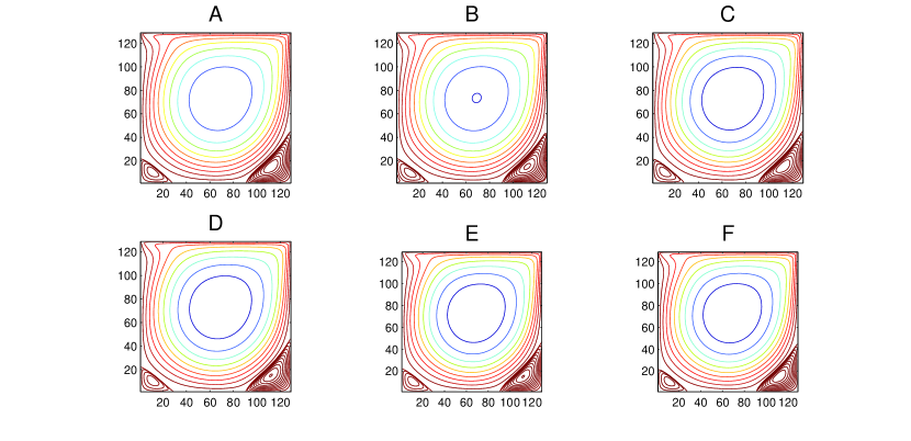
Fig. (4): Contour plots of stream functions of A: BGK, B: BGK + Ehrenfest Steps, C: BGK + MRT Limiter, D: TRT, E: MRT, F: MRT1 following 10000000 time steps at Re1000.

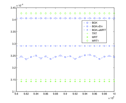
Fig. (5): Enstrophy in the Re1000 systems during the final $2\cdot 10^{5}$ time steps

All of these systems are stable for Re1000, the contour plots of the final state are given in Figure (4) and there appears only small differences. We calculate the average enstrophy in each system and plot it as a function of time in Figure (5). We can see that in the different systems that enstrophy and hence dissipation varies. Compared with the BGK system all the other systems except MRT1 exhibit a lower level of enstrophy indicating a higher rate of dissipation. For MRT1 the fixed relaxation rate of the third order mode is actually less dissipative than the BGK relaxation rate for this Reynolds number, hence the increased enstrophy. An artifact of using the pointwise filtering techniques is that they introduce small scale local oscillations in the modes that they regularize, therefore the system seems not to be asymptotically stable. This might be remedied by increasing the threshold of $\Delta S$ below which no regularization is performed. Nevertheless in these experiments after sufficient time the enstrophy values remain within a small enough boundary for the results to be useful.

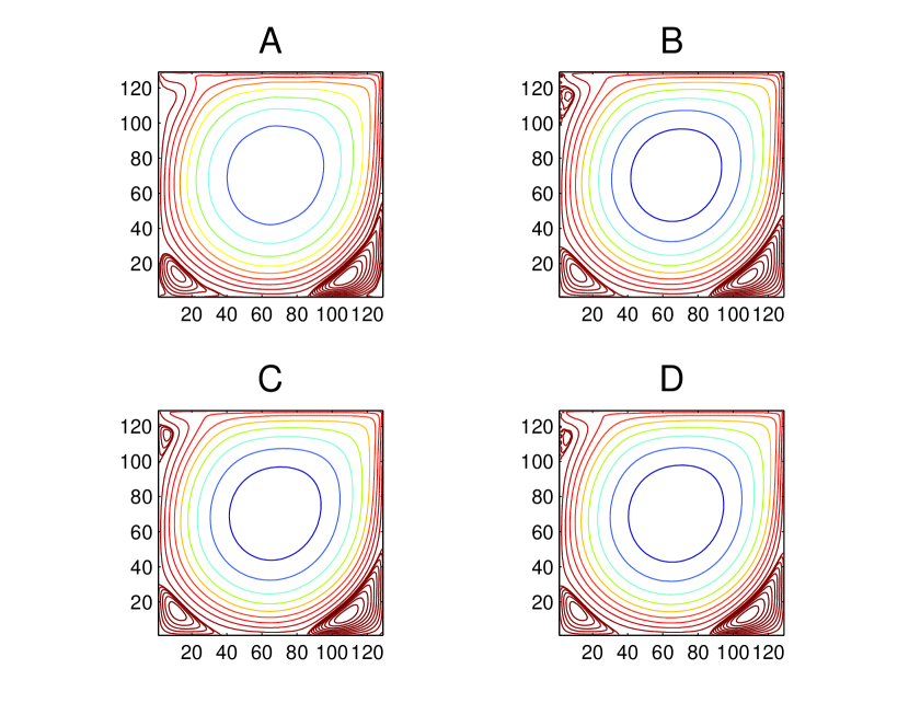
Fig. (6): Contour plots of stream functions of A: BGK + Ehrenfest Steps, B: BGK + MRT Limiter, C: TRT, D: MRT1,following 10000000 time steps at Re2500.

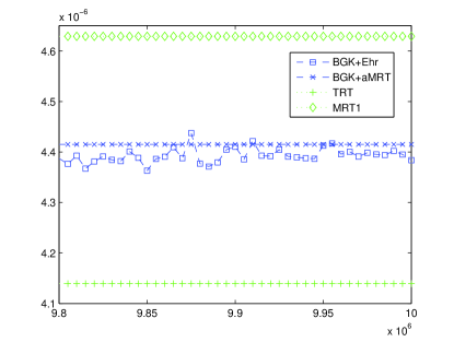
Fig. (7): Enstrophy in the Re2500 systems during the final $2\cdot 10^{5}$ time steps

The next Reynolds number we choose is Re2500. Only 4 of the original 6 systems complete the full number of time steps for this Reynolds number, the contour plots of the final stream functions are given in Figure (6). Of the systems which did not complete the simulation it should be said that the MRT system survived a few 10s of thousands of time steps while the BGK system diverged almost immediately, indicating that it does provide stability benefits which are not apparent at the coarse granularity of Reynolds numbers used in this study. One feature to observe in the stream function plots is the absence of an upper left vortex in the Ehrenfest limiter. This system selects the "most non-equilibrium" sites to apply the filter. These typically occur near the corners of the moving lid. It seems here that the local increase in shear viscosity is enough to prevent this vortex forming. This problem does not seem to affect the MRT limiter which preserves the correct production of shear viscosity.

Again we check the enstrophy of the systems and give the results for the final timesteps in Figure (7). Due to the failure of the BGK system to complete this simulation there is no "standard" result to compare the improved methods with. The surviving methods maintain their relative positions with respect to enstrophy production.

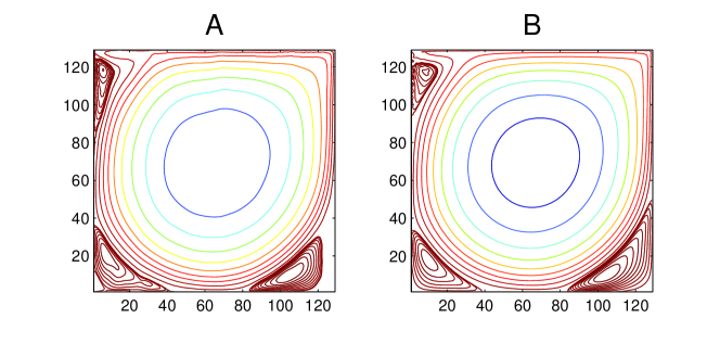
Fig. (8): Contour plots of stream functions of A: BGK + Ehrenfest Steps, B: MRT1,following 10000000 time steps at Re5000.

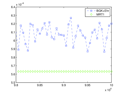
Fig. (9): Enstrophy in the Re5000 systems during the final $2\cdot 10^{5}$ time steps

For the theoretical Reynolds number of 5000 only two systems remain, their streamfunction plots are given in Figure (8). At this Reynolds number the upper left vortex has appeared in the Ehrenfest limited simulation, however a new discrepancy has arisen. The lower right corner exhibits a very low level of streaming.

In Figure (9) the enstrophy during the final parts of the simulation is given. We note that for the first time the MRT1 system produces less enstrophy (is more dissipative) than the BGK system with Ehrenfest limiter.

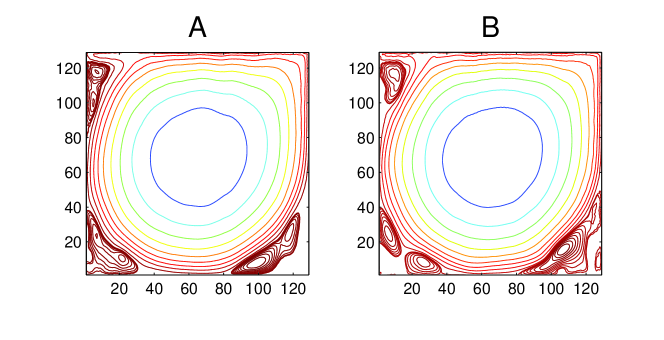
Fig. (10): Contour plots of stream functions of A: Re7500 and B: Re10000 BGK + Ehrenfest systems,following 10000000 time steps at Re5000.

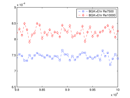
Fig. (11): Enstrophy in the Re7500 and Re10000 BGK + Ehrenfest systems during the final $2\cdot 10^{5}$ time steps

For the final two Reynolds numbers we use, 7500 and 10000, only the BGK system with the Ehrenfest limiter completes the simulation. The corresponding streamfunction plots are given in Figure (10) and they exhibit multiple vortices in the corners of the domain.

The enstrophy plots are given in Figure (11), as the theoretical Reynolds number increases so does the level of enstrophy.

8.2. First Hopf Bifurcation

As Reynolds number increases the flow in the cavity is no longer steady and a more complicated flow pattern emerges. On the way to a fully developed turbulent flow, the lid-driven cavity flow is known to undergo a series of period doubling Hopf bifurcations.

A survey of available literature reveals that the precise value of $\mathrm{Re}$ at which the first Hopf bifurcation occurs is somewhat contentious, with most current studies (all of which are for incompressible flow) ranging from around $\mathrm{Re}=7400$–$8500$ [6, 27, 28]. Here, we do not intend to give a precise value because it is a well observed grid effect that the critical Reynolds number increases (shifts to the right) with refinement (see, e.g., Fig. 3 in [28]). Rather, we will be content to localise the first bifurcation and, in doing so, demonstrate that limiters are capable of regularising without effecting fundamental flow features.

To localise the first bifurcation we take the following algorithmic approach. Entropic equilibria are in use. The initial uniform fluid density profile is $\rho=1.0$ and the velocity of the lid is $u_{0}=1/10$ (in lattice units). We record the unsteady velocity data at a single control point with coordinates $(L/16,13L/16)$ and run the simulation for $5000L/u_{0}$ time steps. Let us denote the final 1% of this signal by $(u_{\mathrm{sig}},v_{\mathrm{sig}})$. We then compute the energy $E_{u}$ ($\ell_{2}$-norm normalised by non-dimensional signal duration) of the deviation of $u_{\mathrm{sig}}$ from its mean:

$$E_{u}:=\biggl{\|}\sqrt{\frac{L}{u_{0}|u_{\mathrm{sig}}|}}(u_{\mathrm{sig}}-\overline{u_{\mathrm{sig}}})\biggr{\|}_{\ell_{2}},$$ (34)

where $|u_{\mathrm{sig}}|$ and $\overline{u_{\mathrm{sig}}}$ denote the length and mean of $u_{\mathrm{sig}}$, respectively. We choose this robust statistic instead of attempting to measure signal amplitude because of numerical noise in the LBM simulation. The source of noise in LBM is attributed to the existence of an inherently unavoidable neutral stability direction in the numerical scheme (see, e.g., [3]).

We opt not to employ the “bounce-back” boundary condition used in the previous steady state study. Instead we will use the diffusive Maxwell boundary condition (see, e.g., [8]), which was first applied to LBM in [2]. The essence of the condition is that populations reaching a boundary are reflected, proportional to equilibrium, such that mass-balance (in the bulk) and detail-balance are achieved. The boundary condition coincides with “bounce-back” in each corner of the cavity.

To illustrate, immediately following the advection of populations consider the situation of a wall, aligned with the lattice, moving with velocity $u_{\mathrm{wall}}$ and with outward pointing normal to the wall in the negative $y$-direction (this is the situation on the lid of the cavity with $u_{\mathrm{wall}}=u_{0}$). The implementation of the diffusive Maxwell boundary condition at a boundary site $(x,y)$ on this wall consists of the update

$$f_{i}(x,y,t+1)=\gamma f^{*}_{i}(u_{\mathrm{wall}}),\qquad i=4,7,8,$$

with

$$\gamma=\frac{f_{2}(x,y,t)+f_{5}(x,y,t)+f_{6}(x,y,t)}{f^{*}_{4}(u_{\mathrm{wall}})+f^{*}_{7}(u_{\mathrm{wall}})+f^{*}_{8}(u_{\mathrm{wall}})}.$$

Observe that, because density is a linear factor of the equilibria, the density of the wall is inconsequential in the boundary condition and can therefore be taken as unity for convenience. As is usual, only those populations pointing in to the fluid at a boundary site are updated. Boundary sites do not undergo the collisional step that the bulk of the sites are subjected to.

We prefer the diffusive boundary condition over the often preferred “bounce-back” boundary condition with constant lid profile. This is because we have experienced difficulty in separating the aforementioned numerical noise from the genuine signal at a single control point using “bounce-back”. We remark that the diffusive boundary condition does not prevent unregularised LBGK from failing at some critical Reynolds number.

Now, we conduct an experiment and record (34) over a range of Reynolds numbers. In each case the median filter limiter is employed with parameter $\delta=10^{-3}$. Since the transition between steady and periodic flow in the lid-driven cavity is known to belong to the class of standard Hopf bifurcations we are assured that $E_{u}^{2}\propto\mathrm{Re}$ [12]. Fitting a line of best fit to the resulting data localises the first bifurcation in the lid-driven cavity flow to $\mathrm{Re}=7135$ (Fig. (12)). This value is within the tolerance of $\mathrm{Re}=7402\pm 4\%$ given in [28] for a $100\times 100$ grid. We also provide a (time averaged) phase space trajectory and Fourier spectrum for $\mathrm{Re}=7375$ at the monitoring point (Fig. (13) and Fig. (14)) which clearly indicate that the first bifurcation has been observed.

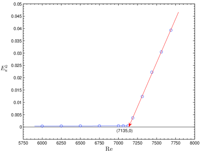
Fig. (12): Plot of energy squared, $E_{u}^{2}$ (34), as a function of Reynolds number, $\mathrm{Re}$, using LBGK regularised with the median filter limiter with $\delta=10^{-3}$ on a $100\times 100$ grid. Straight lines are lines of best fit. The intersection of the sloping line with the $x$-axis occurs close to $\mathrm{Re}=7135$.

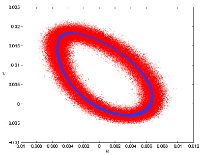
Fig. (13): A phase trajectory for velocity components for the signal $(u_{\mathrm{sig}},v_{\mathrm{sig}})$ at the monitoring point $(L/16,13L/16)$ using LBGK regularised with the median filter limiter with $\delta=10^{-3}$ on a $100\times 100$ grid ($\mathrm{Re}=7375$). Dots represent simulation results at various time moments and the solid line is a $100$ step time average of the signal.

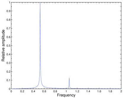
Fig. (14): Relative amplitude spectrum for the signal $u_{\mathrm{sig}}$ at the monitoring point $(L/16,13L/16)$ using LBGK regularised with the median filter limiter with $\delta=10^{-3}$ on a $100\times 100$ grid ($\mathrm{Re}=7375$). We measure a dominant frequency of $\omega=0.525$.

9. CONCLUSION

In the 1D shock tube we do not find any evidence that maintaining the proper balance of entropy (implementing ELBM) regularizes spurious oscillations in the LBM. We note that entropy production controlled by $\alpha$ and viscosity controlled by $\beta$ are composite in the collision integral (6). A weak lower approximation to $\alpha$ would lead effectively to addition of dissipation at the mostly far from equilibrium sites and therefore would locally increase viscosity. Therefore the choice of the method to implement the entropic involution is crucial in this scheme. Any method which is not sufficiently accurate could give a misleading result.

In the 2D lid driven cavity test we observe that implementing TRT[13] or MRT[22] with certain relaxation rates can improve stability. The increase in stability from using TRT can be attributed to the correction of the numerical slip on the boundary, as well as increasing dissipation. What is the best set of parameters to choose for MRT is not a closed question. The parameters used in this work originally proposed by Lallemand and Luo [22] are based on a linear stability analysis. Certain choices of relaxation parameters may improve stability while qualitatively changing the flow, so parameter choices should be justified theoretically, or alternatively the results of simulations should be somehow validated. Nevertheless the parameters used in this work exhibit an improvement in stability over the standard BGK system.

Modifying the relaxation rates of the different modes changes the production of dissipation of different components at different orders of the dynamics. The higher order dynamics of latttice Boltzmann methods include higher order space derivatives of the distribution functions. MRT could exhibit the very nice property that where these derivatives are near to zero that MRT has little effect, while where these derivatives are large (near shocks and oscillations) that additional dissipation could be added, regularizing the system.

Using entropic limiters explicitly adds dissipation locally[4]. The Ehrenfest steps succeed to stabilize the system at Reynolds numbers where other tested methods fail, at the cost of the smoothness of the flow. We also implemented an entropic limiter using MRT technology. This also succeeded in stabilizing the system to a degree, however the amount of dissipation added is less than an Ehrenfest step and hence it is less effective. The particular advantage of a limiter of this type over the Ehrenfest step is that it can preserve the correct production of dissipation on physical modes across the system. Other MRT type limiters can easily be invented by simply varying the relaxation parameters.

As previously mentioned there have been more filtering operations proposed[29]. These have a similar idea of local (but not pointwise) filtering of lattice Boltzmann simulations. A greater variety of variables to filter have been examined, for example the macroscopic field can be filtered rather than the mesoscopic population functions.

We can use the Enstrophy statistic to measure effective dissipation in the system. The results from the lid-driven cavity experiment indicate that increased total dissipation does not necessarily increase stability. The increase in dissipation needs to be targeted onto specific parts of the domain or specific modes of the dynamics to be effective.

Using the global median filter in the lid-driven cavity we find that the expected Reynolds number of the first Hopf bifurcation seems to be preserved, despite the additional dissipation. This is an extremely positive result as it indicates that if the addition of dissipation needed to stabilize the system is added in an appropriate manner then qualitative features of the flow can be preserved.

Finally we should note that the stability of lattice Boltzmann systems depends on more than one parameter. In all these numerical tests the Reynolds number was modified by altering the rate of production of shear viscosity. In particular, for the lid driven cavity the Reynolds number could be varied by altering the lid speed, which was fixed at 0.1 in all of these simulations. Since the different modes of the dynamics include varying powers of velocity, this would affect the stability of the system in a different manner to simply changing the shear viscosity coefficient. In such systems the relative improvements offered by these methods over the BGK system could be different.

The various LBMs all work well in regimes where the macroscopic fields are smooth. Each method has its limitation as they attempt to simulate flows with, for example, shocks and turbulence, and it is clear that something needs to be done in order to simulate beyond these limitations. We have examined various add-ons to well-known implementations of the LBM, and explored their efficiency. We demonstrate that add-ons based on the gentle modification of dissipation can significantly expand the stable boundary of operation of the LBM.

REFERENCES

REFERENCES

- [1] Ansumali S, Karlin IV. Stabilization of the lattice Boltzmann method by the H theorem: A numerical test. Phys Rev E 2000; 62(6): 7999–8003.
- [2] Ansumali S, Karlin IV. Kinetic boundary conditions in the lattice Boltzmann method. Phys Rev E 2002; 66: 026311.
- [3] Brownlee RA, Gorban AN, Levesley J. Stabilisation of the lattice-Boltzmann method using the Ehrenfests’ coarse-graining. Phys Rev E 2006; 74: 037703.
- [4] Brownlee RA, Gorban AN, Levesley J. Stability and stabilisation of the lattice Boltzmann method. Phys Rev E 2007; 75: 036711.
- [5] Brownlee RA, Gorban AN, Levesley J. Nonequilibrium entropy limiters in lattice Boltzmann methods, Physica A 2008; 387: 385–406.
- [6] Bruneau C-H, Saad M. The 2D lid-driven cavity problem revisited. Comput Fluids 2006; 35: 326–348.
- [7] Benzi R., Succi S, Vergassola M. The lattice Boltzmann-equation - theory and applications. Physics Reports 1992; 222(3): 145 197.
- [8] Cercignani C. Theory and application of the Boltzmann equation. Scottish Academic Press, Edinburgh 1975.
- [9] Chen S, Doolen GD. Lattice Boltzmann method for fluid flows. Annu Rev Fluid Mech 1998; 30: 329 364.
- [10] Dellar PJ. Bulck and shear viscosities in lattice Boltzmann equation. Phys Rev E 2001; 64: 031203.
- [11] Dellar PJ. Incompressible limits of lattice Boltzmann equations using multiple relaxation times. J Comput Phys 2003; 190: 351–370.
- [12] Ghaddar NK, Korczak KZ, Mikic BB, Patera AT. Numerical investigation of incompressible flow in grooved channels. Part 1. Stability and self-sustained oscillations. J Fluid Mech 1986; 163: 99–127.
- [13] Ginzburg I. Generic boundary conditions for lattice Boltzmann models and their application to advection and anisotropic dispersion equations. Adv Water Res 2005; 28: 1196 1216.
- [14] Godunov SK. A difference scheme for numerical solution of discontinuous solution of hydrodynamic equations. Math Sbornik 1959; 47: 271–306.
- [15] Gorban AN. Basic type of coarse-graining. In: Model Reduction and Coarse-Graining Approaches for Multiscale Phenomena, ed. by AN Gorban, N Kazantzis, IG Kevrekidis, HC Öttinger, C. Theodoropoulos Springer, Berlin-Heidelberg, New York 2006: 117–176.
- [16] Gorban AN, Karlin IV, Öttinger HC, Tatarinova LL. Ehrenfests argument extended to a formalism of nonequilibrium thermodynamics, Physical Review E 2001; 63: 066124.
- [17] Higuera F, Succi S, Benzi R. Lattice gas dynamics with enhanced collisions. Europhys Lett 1989; 9: 345 349.
- [18] Karlin IV, Ferrante A, Öttinger HC. Perfect entropy functions of the Lattice Boltzmann method. Europhys Lett 1999; 47: 182–188.
- [19] Karlin IV, Gorban AN, Succi S, Boffi V. Maximum Entropy Principle for Lattice Kinetic Equations. Phys Rev Lett 1998; 81:6–9 .
- [20] Kullback S. Information theory and statistics. Wiley, New York 1959.
- [21] Kuzmin D, Lohner R, Turek S. Flux Corrected Transport, Springer 2005.
- [22] Lallemand P, Luo LS. Theory of the lattice Boltzmann method: Dispersion, dissipation, isotropy, Galilean invariance, and stability. Phys Rev E 2000; 61(6): 6546-6562.
- [23] Lax PD. On dispersive difference schemes. Physica D 1986; 18: 250–254.
- [24] Levermore CD, Liu J-G. Oscillations arising in numerical experiments, Physica D 1996; 99: 191–216.
- [25] Li Y, Shock R, Zhang R, Chen H. Numerical study of flow past an impulsively started cylinder by the lattice-Boltzmann method. J Fluid Mech 2004; 519: 273–300.
- [26] Luo LS, Liao W, Chen X, Peng Y. and Zhang W. Numerics of the lattice Boltzmann method: Effects of collision models on the lattice Boltzmann simulations. Phys Rev E 2011; 83: 056710.
- [27] Pan TW, Glowinksi R. A projection/wave-like equation method for the numerical simulation of incompressible viscous fluid flow modeled by the Navier–Stokes equations. Comp Fluid Dyn J 2000; 9: 28–42.
- [28] Peng Y-F, Shiau Y-H, Hwang RR. Transition in a 2-D lid-driven cavity flow. Comput Fluids 2003; 32: 337–352.
- [29] Ricot D, Marie S, Sagaut P, Bailly C. Lattice Boltzmann method with selective viscosity filter. J Comput Physics 2009; 228: 4478–4490.
- [30] Pratt WK. Digital Image Processing. Wiley, New York 1978.
- [31] Roy CJ. Grid convergence error analysis for mixed-order numerical schemes. AIAA J 2003; 41: 595–604
- [32] Servan-Camas B, Tsai FT-C. Non-negativity and stability analyses of lattice Boltzmann method for advection diffusion equation. J Comput Physics 2009; 228(1): 236-256
- [33] Succi S. The lattice Boltzmann equation for fluid dynamics and beyond. Oxford University Press, New York 2001.
- [34] Tadmor E, Zhong W. Entropy stable approximations of Navier–Stokes equations with no artificial numerical viscosity. J Hyperbolic DEs 2006; 3: 529–559.
- [35] Tosi F, Ubertini S, Succi S, Chen H, Karlin IV. A comparison of single-time relaxation lattice Boltzmann schemes with enhanced stability. Math Comput Simulation 2006; 72: 227–231.
- [36] Wesseling P. Principles of Computational Fluid Dynamics. Springer Series in Computational Mathematics 29, Springer, Berlin 2001.