Exploration of SFPR techniques for astrometry and observations of weak sources with high frequency Space VLBI.

Abstract

Space Very-Long-Baseline-Interferometry (S-VLBI) observations at high frequencies hold the prospect of achieving the highest angular resolutions and astrometric accuracies, resulting from the long baselines between ground and satellite telescopes. Nevertheless, space-specific issues, such as limited accuracy in the satellite orbit reconstruction and constraints on the satellite antenna pointing operations, limit the application of conventional phase referencing. We investigate the feasibility of an alternative technique, source frequency phase referencing (SFPR), to the S-VLBI domain. With these investigations we aim to contribute to the design of the next-generation of S-VLBI missions. We have used both analytical and simulation studies to characterize the performance of SFPR in S-VLBI observations, applied to astrometry and increased coherence time, and compared these to results obtained using conventional phase referencing. The observing configurations use the specifications of the ASTRO-G mission for their starting point. Our results show that the SFPR technique enables astrometry at 43 GHz, using alternating observations with 22 GHz, regardless of the orbit errors, for most weathers and under a wide variety of conditions. The same applies to the increased coherence time for the detection of weak sources. Our studies show that the capability to carry out simultaneous dual frequency observations enables the application to higher frequencies, and a general improvement of the performance in all cases, hence we recommend its consideration for S-VLBI programs.

1 Introduction

The pursuit of ever higher angular resolution is the driver pushing VLBI observations into higher radio frequency domains, and increasingly larger telescope separations. Advances on both fronts have allowed the mapping of the structure of astronomical objects, such as distant active galactic nuclei (AGN), at steadily increasing resolution. A major step forward is expected from the combination of observations with the longest baselines and at high frequencies, that is, with the next-generation of S-VLBI. This will target a range of fundamental physical problems, such as measuring the properties of accretion disks in super-massive black holes, amongst others (see http://www.vsop.isas.jaxa.jp/vsop2e/science, as well as Takahashi (2004); Takahashi & Mineshige (2011)). Suitable astrometric accuracy and the high sensitivity required to measure these properties are important tools to provide a path to those ends. This paper is concerned with developments of calibration techniques that enable these outcomes, in the light of current and future space missions.

Joint observations between ground radio telescopes and the Japanese satellite HALCA, launched in 1997 (Hirabayashi et al., 2000), demonstrated the feasibility of S-VLBI. HALCA operated at 1.6/5 GHz, mainly for imaging purposes using self-calibration techniques (e.g. Dodson et al. (2009)), and some limited astrometry (Porcas et al., 2000; Guirado et al., 2001). Following this success a number of S-VLBI astronomical projects are currently under development, such as ASTRO-G (Tsuboi, 2009), RadioAstron (Kardashev, 1997), Millimetron (Wild et al., 2009). Their mission specifications comprise a range of orbit apogees from 25,000 to 350,000 km, with most frequencies in the cm and mm range, and satellite antenna diameters in the range 9 to 12 meters. For more detailed information on these missions see the references listed.

The long baselines involved in S-VLBI hold the potential of achieving the highest spatial resolution at any particular frequency. Nevertheless, the requirements for the astrometric capability and enhanced sensitivity that are achieved with conventional phase referencing using ground arrays are difficult to meet with a spacecraft, particularly at the higher frequencies ($>22$ GHz). For example, the astrometric capability strongly depends on the Orbit Determination Discrepancy at Apogee (ODDA) and requires cm-level orbit reconstruction, which is extremely difficult to realize using conventional range and range-rate satellite tracking techniques (Asaki et al., 2008).

Conventional phase referencing analysis (Alef, 1988; Beasley & Conway, 1995) routinely achieves high precision astrometric measurements using observations with ground arrays in the range between 2 and 43 GHz. Its successful implementation is strongly dependent on the existence of a nearby, compact and strong calibrator for alternating observations with the target source, and having accurate a-priori models for the source and antenna positions, and atmospheric effects, amongst others. The rapid source-switching cycles required to compensate for the tropospheric fluctuations at high frequencies, the scarcity of suitable calibrator sources and the constraints on a priori models pose an insurmountable limitation to the application of this technique beyond 43 GHz.

In theory, phase referencing techniques can be applied both to space and ground baselines. In practice, the analysis of HALCA data showed that the calibration of S-VLBI observations involves additional difficulties arising from the lower correlated source flux densities at the higher resolution of space baselines, relatively poor sensitivity achievable with small orbiting antennas, technical difficulties of rapid pointing changes for 10-m class deployable antennas in space and large geometric delay errors introduced by uncertainties in the spacecraft orbit preventing long integration times, and astrometry (Porcas et al., 2000).

Asaki and collaborators (2007) (hereafter A07) have carried out a comprehensive study on the feasibility of conventional phase referencing observations with ASTRO-G, under a range of different weather conditions, such as source separations and orbit determination accuracy of the satellite, among other parameters. Their simulations conclude that astrometrical observations are expected to achieve a good performance at 8.4 GHz, while at higher frequencies the best possible weather would be required and the probability of finding suitable calibrators, particularly at 43 GHz, is greatly reduced. In all cases, cm-level orbit reconstruction is required and additional instruments for precise orbit determination would be needed on board, such as Global Navigation Satellite System navigation, Satellite Laser Ranging, etc. as described in Asaki et al. (2008) and Wu & Bar-Sever (2001).

We propose an alternative phase calibration strategy that widens the astrometric capability and enhances the sensitivity of S-VLBI, by addressing the space-specific and high frequency issues mentioned above. By doing that, it allows the application to many targets and frequencies beyond the limits of conventional phase referencing. The source frequency phase referencing (SFPR hereafter) technique consists of using observations at another (lower) frequency, plus another source to calibrate the target source observations at a higher frequency. The direct astrometric outcome of SFPR observations is high precision bona fide astrometry between frequencies, of interest in studies where the spatial alignment of emission, continuum or spectral line, at multiple frequencies is crucial; when combined with conventional phase referencing (PR hereafter) at the lower frequency, this enables relative astrometry with respect to an external reference at the higher frequency, for proper motion, parallax, and other such studies. The basis of the SFPR strategy is presented in detail in Rioja & Dodson (2011) (RD11 hereafter), and Dodson & Rioja (2009), along with an error analysis, and an empirical demonstration with observations using the VLBA ground array at 43 and 86 GHz. This paper is concerned with its application to S-VLBI, and is a development of the VLBA Memo by Rioja & Dodson (2009). In Section 2 we focus on the advantages and suitability of the SFPR calibration method to provide astrometry and increased coherence for mm-wavelength S-VLBI observations. In Section 3 we present the results from analytical and simulation studies which use the specifications of the ASTRO-G mission as a starting point. Section 4 aims at a more general discussion of S-VLBI, and provides suggestions for design improvements.

2 The SFPR technique and feasibility studies for Space VLBI

2.1 The SFPR technique

The two-step SFPR astrometric calibration approach relies on fast frequency switching, or ideally simultaneous dual frequency observations, combined with slow source switching observations, between two frequencies ($\nu^{high}$ and $\nu^{low}$) and two sources (A and B), respectively. The former step alone provides a method to compensate for the non-dispersive errors in the tropospheric excess delay model, hence effectively increasing the sensitivity of S-VLBI in the high frequency regime, by increasing the coherence time; the orbit determination errors being non-dispersive are compensated in this step as well. When combined with the latter step it enables astrometric capability with S-VLBI irrespective of the uncertainties in the orbit reconstruction, which set an insurmountable limiting factor with PR techniques at high frequencies. Also, since the constraints on a suitable calibrator source are much less severe than in conventional PR, it enables S-VLBI astrometry of many targets at 43 GHz and higher frequencies.

A detailed presentation of the basics of the SFPR technique with ground arrays can be found in RD11. In order to facilitate the reading of this paper we include an extract of the formulae used in RD11, with emphasis on aspects which are specific for S-VLBI. Following standard nomenclature, the residual phase error values for observations of the target source ($A$) at the target frequency, $\phi^{high}_{A}$, are shown as a compound of geometric, tropospheric, ionospheric, instrumental, structural and thermal noise residual terms:

$$\phi^{{\rm high}}_{{\rm A}}=\phi^{{\rm high}}_{{\rm A,geo}}+\phi^{{\rm high}}_{{\rm A,tro}}+\phi^{{\rm high}}_{{\rm A,ion}}+\phi^{{\rm high}}_{{\rm A,inst}}+\phi^{{\rm high}}_{{\rm A,str}}+\phi^{{\rm high}}_{{\rm A,thermal}}+2\pi n^{{\rm high}}_{{\rm A}},\hskip 28.45274ptn^{{\rm high}}_{\rm A}\in{\rm integer},$$ (1)

where $2\pi n^{{\rm high}}_{\rm A}$ stands for the intrinsic phase ambiguity term. $\phi^{{\rm high}}_{{\rm A,str}}$ corresponds to the structure contribution and can be calculated with respect to a feature in the maps. By choosing the “core” component as the phase center the $\phi^{{\rm high}}_{{\rm A,geo}}$ term refers to the position of this “core”. This is the criterion adopted in this paper.

A similar expression to equation (1) holds for the residual phases $\phi^{low}_{A}$ from observations at $\nu^{low}$, the reference frequency. These are analyzed using self-calibration and hybrid imaging techniques so that $\phi_{\rm str}$ is compensated. The resultant antenna-based corrections are linearly interpolated to the times when the $\nu^{high}$ frequency is observed ($\tilde{\phi}^{low}_{A,self-cal}$), scaled by the frequency ratio $R$ (with $R=\frac{\nu^{high}}{\nu^{low}}$), and applied as the calibration for the observed phases at $\nu^{high}$, the target frequency, in equation (1). We name this step as frequency phase transfer (fpt). This calibration strategy results in quasi perfect compensation of non-dispersive residual phase model errors which scale linearly with frequency, such as the tropospheric and geometric contributions, in equation (1). Then, the residual tropospheric contribution is given by:

$$\phi_{{\rm A,tro}}^{{\rm high}}-R\,.\,\tilde{\phi}_{{\rm A,tro}}^{{\rm low}}=\Delta_{{\rm i,T^{\nu}_{\rm swt}}},$$

where $\Delta_{{\rm i,T^{\nu}_{\rm swt}}}$ stands for the interpolation errors arising from using a frequency switching cycle $T^{\nu}_{{\rm swt}}$, which corresponds to the elapsed time between midpoints of two consecutive scans at the same frequency. The propagation in the SFPR analysis is addressed in latter sections. This term can be reduced by selecting a fast frequency switching cycle, matching the properties of the tropospheric fluctuations. Frequency switching is easier than source switching for telescopes in general. The ideal configuration consists of using simultaneous dual frequency observations, for which neither switching nor interpolation is required and $\Delta_{{\rm i,T^{\nu}_{\rm swt}}}$=0.

As for the geometric compensation, it is given by:

$$\phi^{high}_{A,geo}-R\,.\,\tilde{\phi}^{low}_{A,geo}=2\pi\,\vec{D_{\lambda}}\,.\,\vec{\theta_{A}}+O(\vec{\Delta D_{\lambda}}\,.\,\vec{\theta_{A}})\approx 2\pi\,\vec{D_{\lambda}}\,.\,\vec{\theta_{A}}$$ (2)

where $\vec{D_{\lambda}}$ is the baseline vector in units of wavelengths (for $\nu^{high}$), and $\vec{\theta}_{A}$ is the target source position shift between the two observed frequencies. This we refer to as “core shift” by extension of the core shift phenomena in AGNs but also applicable to any spatial spectral shift, independent of its origin. In general, for sources whose VLBI position is frequency dependent, the geometric contribution has a 24-hour sinusoidal term whose amplitude depends on $\vec{\theta}_{A}$. For completeness we include an extra contribution proportional to the scalar product of the antenna position error (or satellite orbit error) and the “core shift” vectors. The effect of the latter extra term is negligible and can be completely ignored given the likely orbit errors, or any other VLBI antenna position errors, and the expected typical values for “core shifts”.

Then, the resultant tropospheric and geometric error-free residuals, so called FPT-calibrated target phases, $\phi_{\rm A}^{{\rm FPT}}$, are:

$$\phi_{\rm A}^{{\rm FPT}}=\phi_{\rm A}^{{\rm high}}-R\,.\,\tilde{\phi}_{{\rm A,self-cal}}^{{\rm low}}=\phi_{{\rm A,str}}^{{\rm high}}+2\pi\,\vec{D_{\lambda}}\,.\,\vec{\theta_{A}}+(\phi_{{\rm A,ion}}^{{\rm high}}-R\,.\,\tilde{\phi}_{{\rm A,ion}}^{{\rm low}})$$

$$+(\phi_{{\rm A,inst}}^{{\rm high}}-R\,.\,\tilde{\phi}_{{\rm A,inst}}^{{\rm low}})+\Delta_{{\rm i,T^{\nu}_{\rm swt}}}$$ (3)

For simplicity we have omitted the noise contribution, and the $2\pi$ phase ambiguity term in Equation 3 which, provided $R$ is an integer value, just adds an unknown number of whole turns and is irrelevant for the analysis. The importance of having an integer ratio between the frequencies involved in SFPR calibration is discussed in RD11; nevertheless, successful analysis using non-integer frequency ratios has been demonstrated (Rioja et al., 2005; Dodson et al., 2011). Also, we take $\phi_{{\rm A,str}}^{{\rm low}}=0$, either because the structure at $\nu^{low}$ has been imaged and corrected for, or it is a compact source. Note that the compensation of the tropospheric short time scale phase variations results in longer coherence times at the higher frequencies $\nu^{high}$, which enables the detection of weaker sources irrespective of the orbit errors. This is of special interest for S-VLBI given the limitations on the size of a satellite antenna and the long baselines. However the remaining dispersive residual phase contributions prevent astrometry.

Interleaving observations of another source B, following the same strategy as for the target source A, offers a way to calibrate the remaining dispersive residual terms in Equation 3. Note that since the remaining ionospheric and instrumental terms show long-scale temporal variations, a slow source switching of several minutes, along with large angular separations of several degrees is feasible. Provided that suitable switching times are used during the observations, the resultant sfpr-visibility phases, $\phi^{{\rm SFPR}}_{{\rm A}}$, are free of the long scale drift terms shown in Equation 3, as:

$$\phi^{{\rm SFPR}}_{{\rm A}}=\phi_{{\rm A,str}}^{{\rm high}}+2\pi\vec{D}_{\lambda}\,.\,(\vec{\theta}_{{\rm A}}-\vec{\theta}_{{\rm B}})+\Delta_{{\rm i,T^{\nu}_{\rm swt}}}+\Delta_{{\rm i,T_{\rm swt}}}$$ (4)

where $\Delta_{{\rm i,T_{\rm swt}}}$ stands for the interpolation errors arising from using a source switching cycle ${\rm T}_{{\rm swt}}$, which corresponds to the elapsed time between midpoints of two consecutive blocks of scans on the same source. The propagation of these interpolation errors in the SFPR analysis is addressed in latter sections. The structure contributions for source B at both frequencies are calculated from the corresponding self-calibration maps, as explained above. The sfpr-calibrated phases are free of geometric, tropospheric, ionospheric and instrumental corruption while keeping the chromatic astrometry signature of frequency dependent position. It is interesting to note that the “core-shift” functional dependence in Equation 4 is identical to that for the pair angular separation in conventional PR, although this method cannot be applied at high frequencies. Finally, a Fourier transformation of the visibilities, without further phase calibration, results in a sfpr-map of the brightness distribution of the target source ($A$) at $\nu^{high}$ frequency, and where the offset of the peak with respect to the center of the map is astrometrically significant: i.e. a measurement of the relative “core shift” between the observed frequencies ($\nu^{high}$ and $\nu^{low}$), for both sources (A and B).

2.2 S-VLBI satellites: ASTRO-G and RadioAstron

Table 1 lists the basic parameters for ASTRO-G and RadioAstron, the best current examples of S-VLBI missions. A full description for the ASTRO-G spacecraft can be found in Tsuboi (2009) and for RadioAstron in Kardashev (1997).

ASTRO-G is equipped with three frequency horns, for X, K and Q bands, each with a slight pointing offset in the optics design. ASTRO-G therefore needs to alter the satellite body attitude in order to switch between observing frequency bands for any particular source. Rapid attitude change can be achieved with the powerful attitude control actuators designed to allow for source switching over angles of $\sim\,3\,$ degrees with a switching period of 1 minute. It is expected that for the very small switching angles required in frequency switching even shorter cycle times could be achieved. Integer frequency ratios exist between the X- and Q-bands and K- and Q-bands of 5 and 2, respectively. For the analytical studies we have also assumed that SFPR observations between X- and K-band are possible, even though an integer ratio does not exist.

RadioAstron was launched on June 18th 2011 on a Zenit-3M launcher and at the time of writing this paper is in checkout phase. It is equipped with 4 frequency receivers in a concentric arrangement, which allows for simultaneous observations of the bands. The frequencies are listed in table 1 and span 1-meter to 1-cm. The maximum antenna slew speed is 3-min/^∘ (RadioAstron SOG, 2010). Based on these specifications, SFPR observations at C/K-bands, with integer frequency ratios of 4 and 5, would be feasible. This is discussed later in this paper, in the context of the large orbit and orbit uncertainties of RadioAstron.

Table 1: Summary of the specifications of two S-VLBI missions. Left) the ASTRO-G satellite and right) the RadioAstron satellite: the orbit, the frequency coverage and the sensitivity. See Tsuboi (2009) and RadioAstron SOG (2010) for more details.

ASTRO-G		RadioAstron
Orbital parameters
Apogee height	25,000 km	Apogee height	350,000 km
Perigee height	1,000 km	Perigee height	25,000 km
Inclination angle	31∘	Inclination angle	51∘
Orbital period	7.5 hr	Orbital period	8.5 days
Observing frequency
X-band	8.0 – 8.8 GHz	P-band	0.320 – 0.328 GHz
K-band	20.6 – 22.6 GHz	L-band	1.64 – 1.69 GHz
Q-band	41.0 – 45.0 GHz	C-band	4.80 – 4.86 GHz
		K-band	18.4 – 25.1 GHz
Antenna sensitivity (SEFD) [Jy]
X-band	6100	P-band	15400
K-band	3600	L-band	2300
Q-band	7550	C-band	4400
		K-band	6500

2.3 An Analytical Study on the Performance of SFPR

A comprehensive analytical study on the propagation of errors in the contributions listed in Equation 1 and in the interpolation processes into SFPR analysis for ground VLBI observations was presented in RD11. Here, we expand this study to include the case of S-VLBI observations. The formulae listed in Table 2 are a slightly modified version of those in RD11, to account for the atmospheric-free orbiting antenna in space-ground baselines (i.e. a factor $\sqrt{2}$ removed). We present the phase residual estimates for four frequency pairs, multiple frequency switching cycles, and typical model errors. The pairs of frequencies were selected to match the capabilities of RadioAstron (4.8/19 GHz) and ASTRO-G (8.4/22 GHz; 22/43 GHz), and explore higher frequency S-VLBI (43/86 GHz). The frequency switching cycles were selected to match the frequency agility of ASTRO-G and VLBA (1 minute) and to explore other regimes (0 minute, 2 minutes).

For comparison we include similar estimates for PR.

Table 2: Formulae for estimating the residual phase errors for a ground-space baseline caused by propagation of errors in the corresponding models, given as subscripts, during the analysis using SFPR techniques, at $\nu^{high}$. The subscripts “A” and “B” stand for the target and calibrator sources, respectively; $\Delta\theta$ stands for the source separation (or switching angle) and $T_{\rm swt}$ is the source switching cycle. The superscripts “high” and “low” stand for the two frequencies $\nu^{high}$ and $\nu^{low}$ observed, respectively, $T^{\nu}_{\rm swt}$ is the frequency switching cycle, $R$ the frequency ratio (${\nu^{high}\over\nu^{low}}$), and $\theta$ stands for the magnitude of the core shift between the two observed frequencies. $D$ is the baseline length, $\Delta P$ represents the combined contribution of Earth Orientation Parameters and antenna position errors, and $\Delta s^{c}$ is the error in the position of the calibrator source. $C_{w}$ describes the weather conditions, with values equal to 1, 2 and 4 for good, typical, and poor tropospheric conditions, respectively. $\Delta l_{z}$ stands for the tropospheric systematic zenith excess path error, and $\Delta I_{v}$ is the ionospheric vertical TEC systematic error. $Z_{g}$, $Z_{i}$ and $Z_{F}$ are the zenith angles which describe the elevation dependence of the atmospheric line-of-sight excess path at different altitudes - for a detailed explanation of these parameters see A07, and RD11.

Error Contributions	SFPR residual phase error
Atmospheric Models:
Dynamic Troposphere	$\sigma\phi^{{\rm high}}_{{\rm dtrp}}[{\rm deg}]\approx R\,27\,C_{w}\,\left({{\rm\nu^{low}}[{\rm GHz}]\over 43{\rm GHz}}\right)\left({\sec{Z_{g}}\over\sec{45^{o}}}\right)^{1/2}\times\left({{\rm T^{\nu}_{\rm swt}}[{\rm s}]\over{\rm 60s}}\right)^{5/6},$
Static Troposphere	$\sigma\phi^{{\rm high}}_{{\rm strp}}[{\rm deg}]\approx R\,76\left({{\rm\nu^{\ low}}[{\rm GHz}]\over 43{\rm GHz}}\right)\left({\Delta l_{z}[{\rm cm}]\over 3{\rm cm}}\right)\left({\theta_{A}[^{0}]\over 2^{o}}\right)\left({\cos{Z_{g}}\over\cos{45^{o}}}\right)^{-1}\left({\tan{Z_{g}}\over\tan{45^{o}}\ }\right)\approx 0,$
Dynamic Ionosphere	$\sigma\phi^{{\rm high}}_{{\rm dion}}[{\rm deg}]\approx\left(R-1/R\right)\,0.46\ \,\left({\sec{Z_{i}}\over\sec{43^{o}}}\right)^{1/2}\left({\nu^{{\rm low}}[{\rm GHz}]\over 43{\rm GHz}}\right)^{-1}\times\left[0.21\left({\rm T_{\rm swt}[s]\over 60s}\right)+\left({\sec{Z_{i}}\over\sec{43^{o}}}\right)\left({\Delta\theta[^{o}]\over 2^{o}}\right)\right]^{\ 5/6},$
Static Ionosphere	$\sigma\phi^{{\rm high}}_{{\rm sion}}[{\rm deg}]\approx\left(R-1/R\right)\,2.7\,\left({\nu^{{\rm low}}[{\rm GHz}]\over 43{\rm GHz}}\right)^{-1}\left({\Delta I_{V}[{\rm TECU}]\over 6{\rm TECU}}\right)\left({\Delta\theta[{\rm deg}]\over 2^{o}}\right)\times\left({\cos{Z_{F}}\over\cos{41^{o}}}\right)^{-1}\left({\tan{Z_{F}}\over\tan{41^{o}}}\right),$
Geometric Models:
Source Position	$\sigma\phi^{{\rm high}}_{{\rm\Delta s}}[{\rm deg}]\approx R\,16\left({\nu^{low}[{\rm GHz}]\over 43{\rm GHz}}\right)\left({\rm D[km]\over 6000km}\right)\left({\Delta s^{c}[{\rm mas}]\over 0.3{\rm mas}}\right)\times\left({\theta_{\rm A}[{\rm deg}]\over 2^{o}}\right)\approx 0,$
Telescope Position	$\sigma\phi^{{\rm high}}_{{\rm bl}}[{\rm deg}]\approx R\,18\left({\nu^{{\rm low}}[{\rm GHz}]\over 43{\rm GHz}}\right)\left({\rm\Delta P[cm]\over 1cm}\right)\times\left({\rm\theta_{A}[deg]\over 2^{o}}\right)\approx 0,$
Others:
Instrumental Contribution	$\sigma\phi^{{\rm high}}_{{\rm inst}}=\left(\phi_{{\rm A,inst}}^{{\rm high}}-R\,.\,\tilde{\phi}_{{\rm\ A,inst}}^{{\rm low}}\right)-\left(\phi_{{\rm B,inst}}^{{\rm high}}-R\,.\,\tilde{\phi}_{{\rm B,inst}}^{{\rm low}}\right)\approx 0,$
Thermal Noise	$\sigma\phi^{{\rm high}}_{{\rm thermal}}=\sqrt{(\sigma\phi^{\nu^{{\rm low}},\nu^{{\rm high}}}_{{\rm A,thermal}})^{2}+(\sigma\phi^{\nu^{{\rm low}},\nu^{{\rm high}}}_{{\rm B,thermal}})^{2}+(\sigma\phi^{\nu{{\rm high}}}_{{\rm A,B,thermal}})^{2}}$

2.4 A Simulation Study on the Performance of SFPR

It has been shown (Pradel et al., 2006; Asaki et al., 2007; Honma et al., 2008) that simple analytical analysis is insufficient for the estimation of astrometric errors in VLBI observations. We have carried out simulation studies to describe the performance of SFPR techniques with S-VLBI observations, both for astrometry and increased sensitivity purposes. The procedure consists of generating synthetic S-VLBI datasets using the ARIS (A07) simulation tool for a given observing configuration and typical values for model errors, as listed in Table 3, and carrying out the SFPR data analysis with AIPS. A detailed description of the models implemented in ARIS can be found in A07; the SFPR analysis with AIPS is described in RD11 and Dodson & Rioja (2009). The outcome of each iteration is a SFPR-map. The figures of merit used to characterize the performance for a set of parameters in ARIS are: the average fractional peak flux recovery, which is the ratio between the map peak and the model source fluxes, and the astrometric error, which is the offset of the peak from the center of the map. Larger values for flux recovery and smaller values for astrometric error quantities are indicative of a better performance. The results for a given observing configuration comprise of multiple simulation cycles, each with a changing relative orientation of the source pair along the four cardinal directions. Each cycle was done with independently generated random values for the tropospheric, ionospheric and geometric parameters.

The results from our SFPR simulation studies are presented in Section 3. Furthermore, the results from these simulations can be extrapolated to other regions of the parameter space, as discussed in Section 4.

Table 3: Region of the Parameter Space explored in our Simulation Studies

Parameter Description	Parameter Values
Space segment	1 satellite antenna with ASTRO-G-like orbit and diameter
Ground segment	a) 10 antennas (the VLBA array)
	b) 6 antennas (sparse non-uniform array, with simultaneous dual frequency capability)
Observing Frequencies	$\nu^{low}=22\,$GHz (K-band); $\nu^{high}=43\,$GHz (Q-band)
Source observing configuration	Source switching angle ($\Delta\theta$) : 0.1, 0.5, 1, 2, 3, 4, 5 degrees
	Source switching cycle ($T_{\rm swt}$): 3,4,6,8,10 minutes
Source Model	Compact structure, S=1 Jansky
Frequency observing configuration	a) Fast frequency switching (T${}^{\nu}_{\rm swt}=1$ minute)
	b) Simultaneous dual frequency observations (T${}^{\nu}_{\rm swt}=0$ sec)
Weather conditions	a) Good ($C_{w}=1$)
	b) Typical ($C_{w}=2$)
	c) Poor ($C_{w}=4$)
Model Errors1	a) ODDA: 2, 4, 6, 8, 16, 32, 64 and 128 cm
	b) ‘Typical’ values for propagation medium:
	($\Delta l_{z}=3$cm; $\Delta I_{v}=6$TECU)
	c) Ground antenna position errors, 1 cm
Studies	a) Astrometry
	b) Phase Coherence

(1): We have used typical values for the parameter model errors, as listed in A07

3 RESULTS

3.1 Analytical Study of SFPR for S-VLBI

Figure 1 shows comparative RMS residual error budgets estimated for PR (Figure 1a) and SFPR (Figure 1b and Figure 1c) applied to S-VLBI observations. The error budgets comprise contributions arising from inaccuracies in the geometric (i.e. satellite orbit and reference source coordinates errors), tropospheric and ionospheric models; these are the dominant sources of errors in a non Signal to Noise Ratio (SNR) limited case. The case of noise dominated observations will be addressed in a future study. The observing configurations are: Figure 1a) for conventional PR observations at 8.4, 22 and 43 GHz with a source switching cycle of 1 minute; Figure 1b) for SFPR observations at four pairs of frequencies ($\nu^{low}/\nu^{high}$), namely, 4.8/19, 8.4/22, 22/43 and 43/86 GHz, with frequency switching cycles T${}^{\nu}_{\rm swt}$ of 1 and 2 minutes, and source switching cycle T_swt of 4 minutes, and Figure 1c) is the same as Figure 1b) but with simultaneous dual frequency observations, i.e. T${}^{\nu}_{\rm swt}$=0. In all cases a source pair angular separation of 2 degrees, a satellite orbit height at apogee of 25,000 km, an orbit error ODDA equal to 10 cm, ‘good’ weather conditions, and typical values for the remaining model errors have been used. The estimated values for SFPR technique have been derived using the formulae in Table 2, and those for conventional PR with the formulae in A07, for a ground-space baseline.

We briefly describe the relative strengths from the individual error contributions in Figure 1 as a function of the observing frequency for each technique. The orbit error is responsible for the largest residual phase contribution using PR techniques, at all frequencies. This is the case for any realistically achievable orbit error, as discussed in A07. The tropospheric errors constitute the next largest contribution, with residuals that are linearly proportional to the observing frequency. Instead, the ionospheric residual contribution is much reduced at 22 and 43 GHz, with respect to that at 8.4 GHz. In the SFPR analysis the effect from the orbit errors is completely compensated, as shown in Figures 1b,c. Using a frequency switching cycle of 1 minute (shown with a solid color bar) the tropospheric (i.e. dynamic) contribution, arising from interpolation errors to the times of the higher frequency observations, is the largest in observations with $\nu^{low}\geq 22$ GHz. This contribution is significantly increased with a frequency switching cycle of 2 minutes (shown with a light gray bar with a color coded outline). At the lower frequency pairs (8.4 to 22 GHz, 4.8 to 19 GHz bands) the ionospheric contribution is dominant. This contribution can be reduced by having a closer pair of sources, while it is independent of the frequency switching cycle. Note that the residual tropospheric contribution in SFPR is smaller than in PR because the static contribution is fully compensated using same line-of-sight observations at the two frequencies. For the case of simultaneous dual frequency SFPR observations (i.e. $T^{\nu}_{\rm swt}$=0) the dynamic tropospheric errors are also fully compensated, leaving only the much smaller (with $\nu^{low}\geq 22$ GHz) ionospheric contribution as shown in 1c. These are typically less than 10% of those from the satellite orbit and tropospheric errors in PR at the highest S-VLBI frequency bands. It is worth mentioning that the analytical studies predict that variations in the source switching cycle in SFPR observations have no significant impact in the RMS estimated residual phase budget; the same applies for variations in the source pair angular separation for the pairs with $\nu^{low}\geq 22$ GHz. The reason being that these affect only the weak ionospheric residuals. Based on these results we proceeded to do a more complete simulation-based investigation.

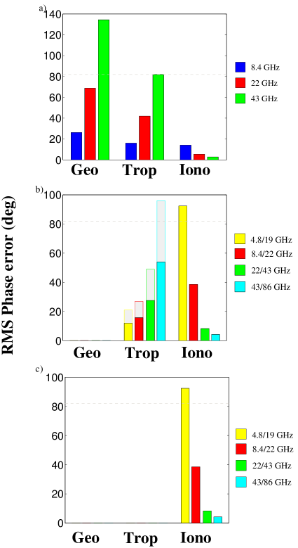
Figure 1: Residual phase error budgets for a S-VLBI baseline for: (a) PR observations at 8.4, 22 and 43 GHz; (b) and (c) SFPR observations at 4.8/19 GHz, 8.4/22 GHz, 22/43 GHz, and 43/86 GHz, estimated with our analytical studies. The plots show the individual contributions arising from typical errors in the geometrical, both for the antenna/orbit and reference source coordinates (Geo), tropospheric (Trop) and ionospheric (Iono) models. The values have been estimated using the formulae in Table 2 at $\nu^{high}$, for SFPR, and in A07, for PR. The PR estimates are for alternating observations of a pair of sources 2 degrees apart, with a switching cycle of 1 minute. For SFPR, we show estimates of two configurations: b) solid bars are for alternating observations between two frequencies, with a switching cycle $T^{\nu}_{\rm swt}$ of 1 minute, of a pair of sources 2 degrees away, with a source switching cycle $T_{\rm swt}$ of 4 minutes; open bars show the same, for a frequency switching cycle of 2 minutes. c) is the same as b), with simultaneous dual frequency observations, i.e. T${}^{\nu}_{\rm swt}=0$. Other relevant parameters which are kept common for all estimates are, satellite ODDA 10 cm, typical tropospheric and ionospheric parameter errors ($\Delta l_{z}\,=\,3\,$cm, $\Delta I_{v}\,=\,6\,$TECU) and good weather conditions. Note the different scales in the vertical axis. The horizontal dashed line in all figures corresponds to the largest tropospheric contribution at 43 GHz in a).

3.2 Simulation Studies for Astrometry with Space VLBI

For our simulation studies we have closely followed the style of the PR feasibility studies for S-VLBI reported in A07, here applied to SFPR. The major effects we wished to explore are the effects of i) frequency switching cycle, ii) weather, iii) source pair angular separation, iv) source switching cycle and v) satellite orbit errors. The frequency switching cycle $T_{\rm swt}^{\nu}=1$ minute, and the observing frequencies ($\nu^{low}=22$, $\nu^{high}=43$ GHz), are compatible with the ASTRO-G mission specifications as well as the VLBA. Full sets of solutions were generated for the whole 2-dimensional grid of source pair switching angles ($\Delta\theta=$ 0.1, 0.5, 1, 2, 3, 4, 5^∘) and source switching cycles ($T_{\rm swt}=$3, 4, 6, 8 and 10 minutes), for fast frequency switching SFPR observations, between 22 and 43 GHz, with $T_{\rm swt}^{\nu}=1$ minute, and for simultaneous dual frequency observations, $T_{\rm swt}^{\nu}=0$. These were repeated for good, typical and poor weather conditions – as defined in A07. The ODDA is 8 cm in all cases, except where otherwise stated. Other parameters were as in A07.

Here we present a subset of these simulations, as the figures of merit were found to have a flat distribution. For the sake of clarity we present two 1-dimensional cuts which fully convey the outcomes. Figure 2 presents the peak flux recovery and the astrometric accuracy quantities through the dataset against all source switching angles, for a source switching cycle of 6 minutes. These results are presented for good (Figure 2a,d), typical (Figure 2b,e) and poor (Figure 2c,f) weather conditions. The figures of merit show no significant variation across this range, with mean values of 86%, 67% and 22% and 1, 1.5 and 2 $\mu$as for good, typical and poor weather, respectively.

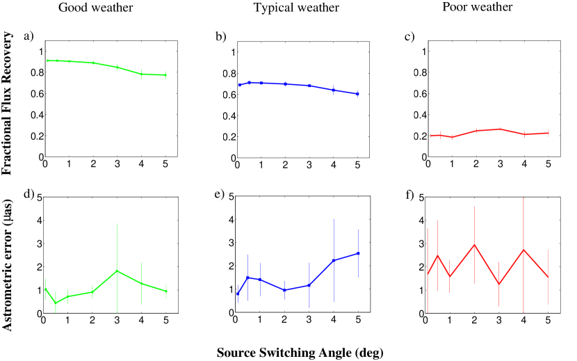
Figure 2: Fractional peak flux recovery (top row: a–c) and astrometric error (bottom row: d–f) quantities as a function of source separation, measured from the SFPR maps at 43 GHz. The results plotted correspond to the mean values of 4 simulations; the error bars are the $\pm$RMS values. Simulations were performed with a frequency switching cycle $T^{\nu}_{\rm swt}$ of 1 minute, a source switching cycle $T_{\rm swt}$ of 6 minutes, ODDA orbit errors of 8 cm and source separations $\Delta\theta$ of 0.1, 0.5, 1, 2, 3, 4 and 5 degrees.

Figure 3a,c) show the one-dimensional cuts through the dataset against all source switching cycles, for a switching angle of 2^∘ and typical weather conditions, showing the fractional peak flux recovery and astrometric error quantities, respectively. Here too, no significant variation is found across the tested range with mean values of 68%, and 0.9 $\mu$as.

Of special relevance for S-VLBI is the propagation of errors in the orbit determination into the astrometric analysis. Figure 3b,d show the figures of merit obtained for ODDA values equal to 2, 4, 8, 16, 32, 64, 128 cm, for SFPR observations of a pair of sources 3 degrees away, using a source switching cycle of 8 minutes, with typical weather conditions. As in previous cases, no significant changes in the values of the figures of merit were seen across the tested range, with mean values of 68% and 1 $\mu$as.

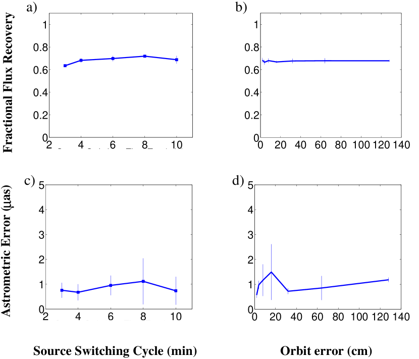
Figure 3: Fractional peak flux recovery (top row: a, b) and astrometric error (bottom row: c, d) quantities as a function of source switching cycle (left: a, c) and ODDA orbit error (right: b, d), measured from the SFPR maps at 43 GHz. The results plotted correspond to the mean values of 4 simulations; the error bars are the $\pm$RMS values. Simulations were performed under typical weather conditions, with a frequency switching cycle $T^{\nu}_{\rm swt}$ of 1 minute. On the left a source separation $\Delta\theta$ of 2^∘, orbit error of 8 cm, and source switching cycles $T_{\rm swt}$ of 3, 4, 6, 8 and 10 minutes. On the right, a source separation $\Delta\theta$ of 3^∘, a source switching cycle of 8 minutes and ODDA orbit errors from 2 to 128 cm, doubling between simulations.

The benefits of carrying out simultaneous dual frequency SFPR observations has been recognized from our previous studies (RD11). Hence, we have included this configuration in our simulations, even though this is not a capability of the ASTRO-G mission nor the VLBA ground array. Thereby we are able to characterize the benefits in comparison with fast frequency switching observations between 22 and 43 GHz. The rest of the parameters for the satellite and ground array antennas were kept the same as in previous simulations. Figure 4 is equivalent to Figure 2, but for simultaneous dual frequency SFPR observations at 22 and 43 GHz. The simulations shown in Figure 4 were carried out using the VLBA as the ground array, for consistency. In this case the flux recovery and astrometric error mean values are 96%, 93% and 83% and 0.6, 0.7 and 1 $\mu$as for good, typical and poor weather, respectively. We also repeated the simulations and confirmed that the results are not significantly different for the case when the VLBA is replaced with a more realistic ground array. This array consisted of antennas that either have, or have expressed plans for, a suitable simultaneous 22/43 GHz receiving system, for example arrays with quasi-optics systems such as the Korean VLBI Network (KVN) (Kim et al., 2007). This realistic ground array was comprised of 6 antennas: 3 KVN antennas (Korea), Yebes-40m (Spain), Effelsberg (Germany) and Shanghai-65m (China).

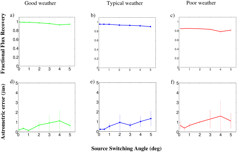
Figure 4: Same as Figure 2, but for simulations using simultaneous dual frequency observations, $T^{\nu}_{\rm swt}=0$.

The choices for T${}^{\nu}_{\rm swt}$ in the simulations was driven by the specifications of the various interferomic arrays discussed. The VLBA/ASTRO-G minimum switching time is 1 minute and for KVN it is 0. Nevertheless, given that the frequency switching time, T${}^{\nu}_{\rm swt}$, and the weather scale factor, $C_{w}$, affect only the dynamic troposphere error contribution, we can combine our simulation results to describe the performance of SFPR observations using frequency switching cycles in the range ca. 0 to 5 minutes, under all weather conditions. Figure 5 shows that, at $\nu^{\rm high}$=43 GHz, frequency switching cycles faster than 0.4, 1.3 and 2.9 minutes are required to maintain fractional peak flux recovery greater than 61%, equivalent to a RMS phase error of 1 radian, for poor, typical and good weather conditions, respectively.

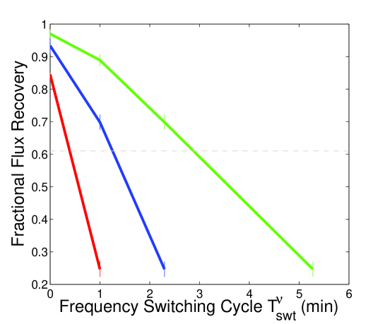
Figure 5: Performance of SFPR observations at 22/43 GHz for a range of frequency switching cycles, under good (right-most line), typical (middle line) and poor (left-most line) weather conditions. In the online version these lines are shown in green, blue and red, respectively. The values in the plot have been derived directly from the simulations, for $T_{\rm swt}^{\nu}$ = 0, 1 minutes, or indirectly, scaling those cycle times by the tropospheric $C_{w}$ parameter raised to the power of 6/5. All simulations have been carried out using $\Delta\theta$=2^∘, ODDA=8 cm and T_swt=6 minutes. The rapid fall in the fractional peak flux recovered for poor weather indicates that a frequency switching cycle faster than 0.4 minutes is required for ‘reliable’ observations. Under typical weather conditions $T^{\nu}_{\rm swt}\leq$ 1.3 minutes are required, while for good weather $T^{\nu}_{\rm swt}\sim$ 2.9 minutes would be acceptable. Based on these results we recommend fast frequency switching cycles of $\sim$ 1 minute for good and typical weathers, and simultaneous dual frequency observations under poor weather conditions, at $\nu^{high}=43$ GHz.

3.3 Simulation Studies for Increased Coherence Time in Space VLBI

We present here the results of our simulation studies to test the feasibility of dual frequency observations to increase the sensitivity of S-VLBI, by increasing the coherence time. We have carried out comparative FPT-calibration simulation studies using fast frequency switching observations with a 1 minute cycle, and simultaneous dual frequency observations, at 22 and 43 GHz, of a single source as described in Section 2.1. Also, for comparison, we carried out simulations using single frequency observations at 43 GHz, followed by self calibration analysis. We used an ODDA orbit error of 8 cm and typical values for the rest of the parameter model errors. All the simulations were carried out for good, typical and poor weather conditions. In all cases, the analysis in AIPS was repeated multiple times using different temporal solution intervals in the task CALIB, from 2 seconds to $\sim$8 hours (in steps doubling the interval) prior to the Fourier inversion to generate the image at 43 GHz. In each case, the fractional peak flux recovery was measured from the image generated using only ground-space baselines.

Figure 6a shows the measured fractional peak flux recovery plotted against the temporal solution interval for the self-calibration analysis case, for all weathers. Taking the usual measure for coherence time as the point where the flux recovery falls below 61% we estimate coherence times for the space to ground baselines of 4, 10 and 20 minutes for poor, typical and good weather respectively.

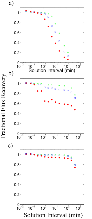
Figure 6: The variation of fractional peak flux recovered as measured from images at 43 GHz as a function of the temporal solution interval in the AIPS task CALIB prior to Fourier inversion of the simulated data. The images have been generated with data from the ground-space baselines only, using different calibration schemes: a) self calibration only; b) FPT-calibration for dual frequency observations at 22 and 43 GHz with a fast frequency switching cycle $T^{\nu}_{\rm swt}$ of 1 minute, followed by self calibration; and, c) same as b), but with simultaneous dual frequency observations, $T^{\nu}_{\rm swt}=0$. All simulations are carried out with an ODDA orbit error of 8 cm, and typical values for the other of model parameter errors. For each case, the three weather conditions are shown: good (stars), typical (squares), and bad (circles). In the online version those are shown in green, blue and red, respectively.

However, if the tropospheric fluctuations, and orbital errors, are compensated using the observations at 22 GHz the coherence time is expected to increase. Figure 6b corresponds to the case of using dual frequency observations with a fast frequency switching cycle of 1 minute, which shows coherence times for good and typical weathers extending to many hours (across the whole simulation run)– which would lead to an order of magnitude improvement of the minimum flux for a detectable source. We find that, unsurprisingly, the poor weather case quickly falls (in 0.5 hours) to a plateau of fractional peak flux recovery around 50–60%, which would cast doubt as to whether this approach would work in poor weather. Finally, the results from simulations using simultaneous dual frequency observations are shown in Figure 6c. In this case, a coherence time up to many hours is estimated under all weather conditions. Note that the remaining long timescale ionospheric and instrumental (i.e. dispersive) residuals using only dual frequency FPT calibration prevents one from achieving astrometry. Also, these are responsible of the decrease in flux observed in Figs 6b and 6c at the longest temporal solution intervals. Using SFPR observations, which include a second source, the flux curve remains flat and also would enable astrometry.

4 Discussion

4.1 Suitability of SFPR for astrometry with S-VLBI

The SFPR technique addresses the issues that limit the application of PR, which works well for ground arrays, to S-VLBI and is a feasible technique to achieve astrometry and enhanced sensitivity even at the highest frequencies. The use of conventional PR calibration techniques for S-VLBI (especially at frequencies $>22$GHz) poses challenges arising from the satellite antenna position errors, which are much larger than for Earth based antennas, and poor sensitivity due to the small orbiting antennas which, in turn, result in the shortage of nearby suitable calibrator sources, plus constraints in satellite operations, i.e. for fast source switching, required to compensate fast tropospheric fluctuations. The SFPR technique compensates for tropospheric and geometric non-dispersive model errors using observations at two frequencies, either with fast frequency switching or simultaneously observed. We have carried out analytical and simulation studies to verify the feasibility of SFPR applied to S-VLBI, both with positive outcomes. Our simulation studies comprise SFPR observations of a satellite antenna with a network of ground telescopes, at 22 and 43 GHz, of compact sources with a range of angular separations between 0.1 to 5 degrees, source switching cycles between 3 and 10 minutes, different weather conditions, and satellite orbit determination discrepancies at apogee (ODDA) ranging from 2 to 128 cm. The simulations are based on the ASTRO-G mission specifications for the satellite antenna, which is capable of frequency switching cycles of 1 minute, except for the subset of simulations with simultaneous dual frequency observations. The ground array was the VLBA, except for the case of simulations with a ‘realistic’ ground array, which was limited to those antennas which support simultaneous dual frequency observations or have plans towards this capability. The analytical studies comprise a wider range of frequencies, starting at 5 GHz to match RadioAstron specifications, and up to 86 GHz.

We use two figures of merit to characterize the performance from the simulations. The fractional peak flux recovery quantity shows an improved performance with shorter frequency switching cycles, especially under poor weather conditions, and for a given cycle, it deteriorates with worsening weather; in comparison it shows little dependence on the pair angular separation or the source switching cycle. The analytical results show that this tendency continues to apply in the tropospheric dominated regime ($\nu^{low}\geq 22$ GHz). Instead, when $\nu^{low}$ is much less than this, the ionospheric errors dominate and increase with pair angular separation. In all cases the performance is independent of the orbit errors.

The results from our simulations show that ‘reliable’ (taken as flux recovery over 61%) astrometric measurements between 22 and 43 GHz at the $\mu$-arcsecond precision level are achievable with SFPR observations with frequency switching cycles $T^{\nu}_{\rm swt}<$ 0.4, 1.3 and 2.9 minutes under poor, typical and good weather conditions, respectively. The astrometric error quantity in our simulations does not vary significantly under the tested conditions, irrespective of the orbit determination error, the angular separation between the two sources $\Delta\theta$, and the source switching cycle $T_{\rm swt}$. This behavior can be easily explained by the two-step strategy of SFPR to compensate errors of different nature. The dynamic tropospheric residuals, which are the dominant contribution if $\nu^{low}\geq 15-22GHz$, are proportional to the frequency switching cycle, as shown in Table 2. The random nature of the residual errors is expected to cause blurring effects in the final SFPR-image, i.e. while the scattering of the phases is expected to decrease the peak flux in the image, the peak will not be shifted from the origin. Only the remaining non-dispersive effects are sensitive to $\Delta\theta$ and $T_{\rm swt}$, and these are weak at the high frequencies of interest here. Therefore, the sfpr route holds great promise for S-VLBI since any orbit errors (as well as ground antennae coordinate errors) are fully removed in the analysis, therefore alleviating the constraint on orbit determination accuracy. This is of importance as the ASTRO-G team has shown that one of the greatest S-VLBI challenges is to accurately measure the antenna position to a few centimeters for a $\sim$ 7-hour long period highly elliptical orbit, with an apogee height of 25,000 km, hence any astrometric approach which could circumnavigate that requirement would be of major benefit. Also, the conditions for a suitable sfpr calibrator source are much more relaxed than in conventional pr, the angular separation between sources can be up to several degrees, and the observing source duty cycle up to several minutes.

4.2 Suitability for detection of weak sources

The SFPR technique offers a technical solution to alleviate the sensitivity issue in S-VLBI observations that arises from the long baselines and small satellite antennas, especially for observations at high frequencies where the coherence time is limited by the rapid tropospheric fluctuations. The requirements for a suitable PR calibrator are increasingly difficult to meet at increasing frequencies in general, and all the more so for S-VLBI. Alternatively, the tropospheric compensation at the target observing frequency can be achieved using detections of the same source at a lower frequency; this results in increased sensitivity at the target frequency. Our simulations characterize the performance of dual frequency tropospheric calibration with S-VLBI at 22 and 43 GHz, using both fast frequency switching (T${}^{\nu}_{\rm swt}$=1min) and simultaneous observations (T${}^{\nu}_{\rm swt}$=0). The results show that increased coherence times up to several hours at 43 GHz (compared to $\sim$ a few minutes of tropospheric coherence times) are achievable under any weather conditions with simultaneous dual frequency observations. More moderate benefits are obtained with fast frequency switching observations. Such an increase in coherence time is equivalent to an increase in sensitivity by a factor of ten. Therefore dual frequency observations enable increased sensitivity for weak sources, one of the major issues for space VLBI, especially at the high frequencies and with very large orbits like RadioAstron. Achieving high sensitivity S-VLBI observations is of paramount importance to address the key science goals of S-VLBI missions.

4.3 Benefits from using simultaneous dual frequency observations

The residual phase error budget in SFPR observations using fast frequency switching is dominated by tropospheric terms, for $\nu^{low}\sim 22$ GHz and higher. For a given frequency switching cycle the tropospheric residual estimates increase linearly with the target frequency $\nu^{high}$ (see formulae in Table 2). This is a result of the imperfect compensation of the rapid tropospheric fluctuations, which requires matching frequency switching times, especially at higher frequencies. Our simulations show that a frequency switching cycle of 1 minute produces high precision astrometric estimates and increased coherence for a wide range of observing configurations at 43 GHz under good and typical weather conditions, but not for poor weather. In this case frequency switching cycles of 0.4 minutes or less are required. At higher frequencies, increasingly faster switching cycles are required even at good and typical weather conditions. The capability for simultaneous dual frequency observations (T${}^{\nu}_{\rm swt}$=0) achieves a perfect tropospheric calibration at any frequency, eliminating the need for fast switching, extending the application of SFPR toward the very high frequency domain. Our analytical studies show its feasibility for observations at 43/86 GHz, and the trend shown in Figure 1c) will continue to be the same at higher frequencies. Therefore, using simultaneous dual frequency SFPR observations allows one to achieve the full potential accuracy of the very precise VLBI phase observable for astrometric measurements, and enables long coherence times under all weather conditions, for both ground and S-VLBI observations even at high frequencies. Hence, we strongly recommend the inclusion of simultaneous dual frequency capability in the mission specifications for future S-VLBI, especially at mm-wavelengths.

4.4 Extrapolation of our results to other regions of parameter space

Our SFPR S-VLBI simulations mainly use the specifications of the ASTRO-G satellite antenna as a starting point, and test a region of the parameter space as described in Table 3. Here we discuss the extrapolation of these results to other missions and regions in the parameter space, namely higher frequencies, different orbits and orbit errors, and aim at extracting information of general interest for S-VLBI. Missions such as RadioAstron, Millimetron and others have been proposed to operate in these domains.

In SFPR observations with RadioAstron at C/K-bands the dominant ionospheric errors are expected to increase with the pair angular separation. In this case, occasional observations of a nearby calibrator, $\leq 1^{\circ}$ away, along with the target source are recommended. The astrometric accuracy is expected to increase if ionospheric errors are kept small. Other than astrometry, we forsee a useful application of FPT observations of the target source to alleviate sensitivity issues at K-band, arising from the expected decrease in the correlated fluxes observed with such a large orbit, using simultaneous observations at C-band to increase the coherence time. Our simulations show the capability of this technique to compensate for errors in the orbit determination. The only requirement on the a-priori orbit determination is set by the delay and rate windows in the correlator processing, for which measurements with errors of a few meters, achievable with conventional satellite tracking techniques, are suitable. Hence, SFPR (and FPT) with RadioAstron, even though $\nu^{low}$ is below the suggested range, will produce significant benefits.

S-VLBI observations up to very high frequencies ($\nu^{high}\geq$ 43 GHz) should be feasible using simultaneous dual frequency observations, even for objects that are too weak to be directly detected, provided they can be detected at a lower frequency $\nu^{low}$. In order to minimize the impact of the ionospheric residual terms, it is recommended to use as a reference frequency $\nu^{low}\sim$15–22 GHz. Intermittent observations, up to tens of minutes, of a distant calibrator, up to several degrees away, should be suitable. The increase in resolving power will result in a parallel increase in the astrometric accuracy, particularly if perfect tropospheric compensation is obtained using simultaneous dual frequency observations, and assuming reasonable SNR values. A study which addresses the case of weak sources and complex structure will be performed in a future series of simulations. In addition, we do not foresee a major impact on the relative performance trends obtained from our simulations. The limit on the highest frequency is not set by the SFPR requirements, but most likely by the surface accuracy required for the satellite antenna. Hence, having simultaneous dual frequency observations improves the performance in all cases, and at frequencies higher than 43 GHz this capability is an imperative.

Ground PR observations beyond 43 GHz are also limited by the rapid tropospheric fluctuations. Here too the use of SFPR techniques would extend the benefits currently achieved with PR to a much higher frequency domain. An early demonstration of the dual frequency calibration step for connected interferometry observations at 19/146 GHz can be found in Asaki et al. (1998). Application of the two step SFPR technique to sub-mm VLBI observations with Atacama Large Millimeter/submillimeter Array (ALMA), for example, is an area of great interest. We are investigating the considerations and requirements for SFPR at the highest frequencies, also in comparison with Water Vapor Radiometer (WVR) phase corrections, and these will be discussed in future publications.

4.5 Outcomes from combining SFPR and PR techniques

The SFPR and PR techniques are complementary in providing astrometric measurements and detection of weak sources in a wide frequency domain and are widely applicable. The direct outcome of SFPR techniques are measurements of the relative separation between the emitting regions at the two observed frequencies, even at mm-wavelengths; this is of direct interest for studies of the core-shift phenomena in AGNs, the alignment of spectral line emission – for example SiO masers at different transitions or from different molecules such as H₂O and SiO – but in general to any position shift regardless of its origin. A07 have shown there is reasonable probability of success of PR observations with S-VLBI for frequencies up to 22 GHz. The combination of astrometric results from SFPR between $\nu^{high}$ and $\nu^{low}$, with conventional PR at the lower frequency $\nu^{low}$, results in astrometric measurements with respect to an external source at $\nu^{high}$, even though conventional PR at $\nu^{high}$ may not be feasible. Therefore, the fields of application mentioned above extend to studies that require the comparison of positions at different epochs, such as proper motion and parallax studies, or stability studies, at the highest frequencies. Hence, the combination of both techniques opens a much larger scope of application, even at high frequencies, with ground and S-VLBI.

5 Conclusions

To summarize, this paper investigates the SFPR technique applied to S-VLBI, to achieve astrometry and increased coherence time for detection of weak sources. Our comprehensive simulation and analytical studies comprise observations between 5 and 86 GHz, either alternated with a switching cycles of 1 and 2 minutes, or simultaneously observed, of pairs of sources with separations up to several degrees, source switching cycles up to many minutes, orbit errors larger than 1 meter, and coherence studies, under all weather conditions. A list of the more significant results obtained from this study is:

1. SFPR solves the specific issues of S-VLBI that limit the application of conventional phase referencing techniques;

2. Our simulations show that $\mu$-arcsecond level astrometry at 43 GHz can be achieved in most cases, using source pair angular separations up to several degrees, and slow source switching cycles with S-VLBI;

3. The satellite antenna orbit error is readily compensated, along with any other non dispersive error, with observations at two frequencies. Hence conventional satellite tracking techniques are sufficient for orbit reconstructions;

4. The same applies to the tropospheric fluctuations which are readily compensated, and result in long coherence times up to several hours. Hence weaker sources can be targeted;

5. The capability for simultaneous dual frequency SFPR observations with S-VLBI is mandatory at $\nu^{high}\geq 43$ GHz, improves the performance at any frequency, and eliminates fast frequency switching operations. Hence this is a crucial capability to include in future mission specifications. At 22/43 GHz, frequency switching cycles faster than approximately 0.4 and 1 minutes, for poor and other weather conditions, respectively, are required;

6. RadioAstron specifications are compatible with SFPR observations, with $\nu^{low}$ of 5 GHz. They are expected to be dominated by ionospheric errors, hence a small source pair angular separation ($\sim 1^{\circ}$) is recommended.

7. Ground VLBI also would benefit from simultaneous dual frequency capability at the highest frequencies observed, especially for compensating tropospheric fluctuations and enabling detection of weaker sources.

6 Acknowledgements

The authors acknowledge support by The University of Western Australia (UWA) to complete this publication, through the Research Collaboration Awards 2009 Round 2 funding program for the project “Enabling state-of-the-art Astrometry with the Japanese Space Mission VSOP-2”.

References

- Alef (1988) Alef, W. 1988, in IAU Symposium, Vol. 129, The Impact of VLBI on Astrophysics and Geophysics, ed. M. J. Reid & J. M. Moran, 523
- Asaki et al. (1998) Asaki, Y., Shibata, K. M., Kawabe, R., Roh, D.-G., Saito, M., Morita, K.-I., & Sasao, T. 1998, Radio Science, 33, 1297
- Asaki et al. (2007) Asaki, Y., et al. 2007, PASJ, 59, 397
- Asaki et al. (2008) Asaki, Y., Takeuchi, H., & Yoshikawa, M. 2008, in Proceedings of the 21st International Technical Meeting of the Satellite Division of The Institute of Navigation (ION GNSS 2008), 710
- Beasley & Conway (1995) Beasley, A. J., & Conway, J. E. 1995, in Astronomical Society of the Pacific Conference Series, Vol. 82, Very Long Baseline Interferometry and the VLBA, ed. J. A. Zensus, P. J. Diamond, & P. J. Napier, 327
- Dodson et al. (2009) Dodson, R., et al. 2008, ApJS, 175, 314
- Dodson & Rioja (2009) Dodson, R., & Rioja, M. 2009, Astrometric Calibration of mm-VLBI Using Source Frequency Phase Referenced Observations (VLBA Scientific Memo), #31
- Dodson et al. (2011) Dodson, R., Rioja, M., & Jung, T. 2011, in 4th East Asia VLBI Meeting
- Guirado et al. (2001) Guirado, J. C., Ros, E., Jones, D. L., Lestrade, J.-F., Marcaide, J. M., Pérez-Torres, M. A., & Preston, R. A. 2001, A&A, 371, 766
- Hirabayashi et al. (2000) Hirabayashi, H., et al. 2000, PASJ, 52, 955
- Honma et al. (2008) Honma, M., Tamura, Y., & Reid, M. J. 2008, PASJ, 60, 951
- Kardashev (1997) Kardashev, N. S. 1997, Experimental Astronomy, 7, 329
- Kim et al. (2007) Kim, H.-G., Han, S.-T., & Sohn, B. W. 2007, The Korean VLBI Network Project, ed. Lobanov, A. P., Zensus, J. A., Cesarsky, C., & Diamond, P. J. (Springer-Verlag), 41
- Pradel et al. (2006) Pradel, N., Charlot, P., & Lestrade, J.-F. 2006, A&A, 452, 1099
- Porcas et al. (2000) Porcas, R. W., Rioja, M. J., Machalski, J., & Hirabayashi, H. 2000, in Astrophysical Phenomena Revealed by Space VLBI, ed. H. Hirabayashi, P. G. Edwards, & D. W. Murphy, 245
- RadioAstron SOG (2010) RadioAstron Science Operations Group, RadioAstron User Handbook http://www.asc.rssi.ru/radioastron/documents/rauh/en/rauh.pdf
- Rioja & Dodson (2009) Rioja, M., & Dodson, R. 2009, Multi-frequency Astrometry with VSOP-2: An Application of Source/Frequency Phase Referencing techniques (VLBA Scientific Memo), #32
- Rioja & Dodson (2011) Rioja, M., & Dodson, R. 2011, AJ, 141, 114
- Rioja et al. (2005) Rioja, M. J., Dodson, R., Porcas, R. W., Suda, H., & Colomer, F. 2005, in Proceedings of 17th Working Meeting on European VLBI for Geodesy and Astrometry
- Takahashi (2004) Takahashi, R. 2004, ApJ, 611, 996
- Takahashi & Mineshige (2011) Takahashi, R., & Mineshige, S. 2011, ApJ, 729, 86
- Tsuboi (2009) Tsuboi, M. 2009, in Astronomical Society of the Pacific Conference Series, Vol. 402, Approaching Micro-Arcsecond Resolution with VSOP-2: Astrophysics and Technologies, ed. Y. Hagiwara, E. Fomalont, M. Tsuboi, & M. Yasuhiro, 30
- Wild et al. (2009) Wild, W., et al. 2009, Experimental Astronomy, 23, 221
- Wu & Bar-Sever (2001) Wu, S.-C., & Bar-Sever, Y. 2001, in Proceedings of the 14th International Technical Meeting of the Satellite Division of The Institute of Navigation (ION GNSS 2001), 2272