Face Recognition using Optimal Representation Ensemble

Abstract

Recently, the face recognizers based on linear representations have been shown to deliver state-of-the-art performance. These approaches assume that the faces, belonging to one individual, reside in a linear-subspace with a respectively low dimensionality. In real-world applications, however, face images usually suffer from expressions, disguises and random occlusions. The problematic facial parts undermine the validity of the subspace assumption and thus the recognition performance deteriorates significantly. In this work, we address the problem in a learning-inference-mixed fashion. By observing that the linear-subspace assumption is more reliable on certain face patches rather than on the holistic face, some Bayesian Patch Representations (BPRs) are randomly generated and interpreted according to the Bayes’ theory. We then train an ensemble model over the patch-representations by minimizing the empirical risk w.r.t. the “leave-one-out margins”. The obtained model is termed Optimal Representation Ensemble (ORE), since it guarantees the optimality from the perspective of Empirical Risk Minimization. To handle the unknown patterns in test faces, a robust version of BPR is proposed by taking the non-face category into consideration. Equipped with the Robust-BPRs, the inference ability of ORE is increased dramatically and several record-breaking accuracies ($99.9\%$ on Yale-B and $99.5\%$ on AR) and desirable efficiencies (below $20$ ms per face in Matlab) are achieved. It also overwhelms other modular heuristics on the faces with random occlusions, extreme expressions and disguises. Furthermore, to accommodate immense BPRs sets, a boosting-like algorithm is also derived. The boosted model, a.k.a. Boosted-ORE, obtains similar performance to its prototype. Besides the empirical superiorities, two desirable features of the proposed methods, namely, the training-determined model-selection and the data-weight-free boosting procedure, are also theoretically verified. They reduce the training complexity immensely, while keeps the generalization capacity not changed.

1 Introduction

Face Recognition is a long-standing problem in computer vision. In the past decade, much effort has been devoted to the Linear Representation (LR) based algorithms such as Nearest Feature Line (NFL) [1], Nearest Feature Subspace (NFS) [2], Sparse Representation Classification (SRC) [3] and the most recently proposed Linear Regression Classification (LRC) [4]. Compared with traditional face recognition approaches, higher accuracies have been reported. The underlying assumption for the LR-classifiers is that the faces of one individual reside in a low-dimensional linear manifold. This assumption, however, is only valid when the cropped faces are considered as rigid Lambertian surfaces and without any occlusion [5, 6]. In practice, the linear-subspace model is sometimes too rudimentary to handle expressions, disguises and random occlusions which usually occur in local regions, e.g. expressions influence the mouth and eyes more greatly than the nose, scarves typically have the impact on lower-half faces. The problematic face parts are not suitable for performing the linear representation and thus reduce the recognition accuracy. On the other hand, there should be some face parts which are less problematic, i.e. more reliable. But, how can we evaluate the reliability of one face part? Given the reliabilities of all the parts, how do we make the final decision?

Several heuristic methods were introduced to address the problem. In particular, the modular approach is used in [3] and [4] for eliminating the adverse impact of continuous occlusions. Significant improvement in accuracy was observed from the partition-and-vote [3] or the partition-and-compete [4] strategy. The drawbacks of these heuristics are also clear. First, one must roughly know a priori the shape and location of the occlusion otherwise the performance will still deteriorate. It is desirable to design more flexible “models” to handle occlusions with arbitrary spatial features. Furthermore, the existing heuristics discard much useful information, like the representation residuals in [3] or the classification results of the unselected blocks in [4]. Higher efficiencies are expected when all the information is simultaneously analyzed. Thirdly, there is great potential to increase the performance by employing a sophisticated fusion method, rather than the primitive rules in [3] and [4]. Finally, most existing methods neglect the fact that the LR-method can also be used to distinguish human faces from non-face images, or partly-non-face images. By harnessing this power, one could achieve higher robustness to occlusions and noises.

In this paper, we propose a learning-inference-mixed framework to learn and recognize faces. The novel framework generate, interpret and aggregate the partial representations more elegantly. First of all, LRs are performed on randomly-generated face patches. Secondly, in a novel manner, we interpret every patch representation as a probability vector, with each element corresponding to a certain individual. The interpretation is obtained via applying Bayes theorem on a basic distribution assumption, and thus is referred to as Bayesian Patch Representation (BPR). We then learn a linear combination of the obtained BPRs to gain much higher classification ability. The combination coefficients, i.e. the weights associated with different BPRs, are achieved via minimizing the exponential loss w.r.t. sample margins [7]. In this way, most given face-related patterns are learned via assigning different “importances” to various patches. The learned model is termed Optimal Representation Ensemble (ORE) since it guarantees the optimality from the perspective of Empirical Risk Minimization. To cope with unknown-patterns in test faces, a variation of BPR, namely Robust-BPR, is derived by taking account of the Generic-Face-Confidence. The inference power of the ORE model is improved dramatically by employing the Robust-BPRs.

The BPRs are, essentially, instance-based. One can not simply copy the off-the-shelf ensemble learning method to combine them. To accommodate the instance-based predictors and optimally exploit the given information, we propose the leave-one-out margin for replacing the conventional margin concept. The leave-one-out margin also makes the ORE-Learning procedure extremely resistant to the overfitting, as we theoretically verified. One therefore can choose the model parameter merely depending on the training errors. This merit of ORE-Learning leads to a remarkable drop in the validation complexity. In addition, to tailor the proposed method to immense BPR sets, a boosting-like algorithm is designed to obtain the ORE in an iterative fashion. The boosted model, Boosted-ORE, could be learned very efficiently as we prove that the training procedure is unrelated to data weights. From a higher point of view, we offer an elegant and efficient framework for training a discriminative ensemble of instance-based classifiers.

A few work has used ensemble learning methods for face recognition [8, 9, 10, 11, 12]. Nonetheless, those methods only combine the model-based, primitive classifiers, e.g. Linear Discriminant Analysis (LDA) or Principle Component Analysis (PCA), which are sensitive to illumination, easy to over-fit and neglect the non-face category. In contrast, our Bayesian-rule-based BPRs overcome all these drawbacks. Furthermore, the proposed ensemble methods globally minimize an explicit loss function w.r.t. margins. It serves as a more principled way, in comparison to the simple voting strategies [8, 9, 12] or the heuristically customized boosting schemes [10, 11].

The experiment part justifies the excellence of proposed algorithms over conventional LR-methods. In particular, ORE achieves some record-breaking accuracies ($99.9\%$ for Yale-B dataset and $99.5\%$ for AR dataset) on the faces with extreme illumination changes, expressions and disguises. Boosted-ORE also shows similar recognition capability. Equipped with the GFC, Robust-ORE outperforms other modular heuristics under all the circumstances. Moreover, the ORE-model also shows the highest efficiency (below $20$ ms per face with Matlab and one CPU core) among all the compared LR-methods.

The rest of this paper is organized as follows. In Section 2, we briefly introduce the family of LR-classifiers and the modular heuristics. BPR and Robust-BPR are proposed in the following section. The learning algorithm for obtaining ORE is derived in Section 4 where we also prove the validity of the training-determined model-selection. The derivations of the boosting-like variation, a.k.a. Boosted-ORE, and its desirable feature in terms of ultrafast training are given in Section 5. Section 6 introduces the learning-inference-mixed strategy of the ORE algorithm. The experiment and results are shown in Section 7 while the conclusion and future topics can be found in the final section.

2 Background

2.1 The family of LR-classifiers

For a face recognition problem, one is usually given $N$ vectorized face images ${\mathbf{X}}\in{\mathbb{R}}^{D\times N}$ belonging to $K$ different individuals, where $D$ is the dimensionality of faces and $N$ is the face number. Let us suppose their labels are ${\mathbf{l}}=\{l_{1},l_{2},\cdots,l_{N}\},$ $l_{i}\in\{1,2,\cdots,K\}~{}\forall i$. When a probe face ${\mathbf{y}}\in{\mathbb{R}}^{D}$ is provided, we need to identify it as one individual exists in the training set, i.e. $\gamma_{{\mathbf{y}}}=H({\mathbf{y}})\in\{1,2,\dots,K\}$, where $H(\cdot)$ is the face recognizer that generates the predicted label $\gamma$. Without loss of generality, in this paper, we assume all the classes share the same sample number $M=N/K$. For the $k$th face category, let ${\mathbf{x}}^{k}_{i}\in{\mathbb{R}}^{D}$ denote the $i$th face image and ${\mathbf{X}}_{k}=[{\mathbf{x}}_{1},{\mathbf{x}}_{2},\dots,{\mathbf{x}}_{M}]\in{\mathbb{R}}^{D\times M}$ indicates the image collection of the $k$th class.

Nearest Neighbor (NN) can be thought of as the most primitive LR-method. It uses only one training face, a.k.a. the nearest neighbor, to represent the test face. However, without a powerful feature extraction approach, NN usually performs very poorly. Therefore, more advanced methods like NFL [1], NFS [2], SRC [3] and LRC [4] are proposed. Most of their formulations ([1, 2, 4]) could be unified. For class $k\in\{1,2,\cdots,K\}$, a typical LR-classifier firstly solve the following problem to get the representation coefficients ${\boldsymbol{\beta}}^{\ast}_{k}$, i.e.

$$\min_{{\boldsymbol{\beta}}_{k}}~{}\|{\mathbf{y}}-\tilde{{\mathbf{X}}}_{k}{\boldsymbol{\beta}}_{k}\|_{2}~{}~{}\forall~{}k\in\{1,2,\cdots,K\},$$ (1)

where $\|\cdot\|_{p}$ stands for the $\ell_{p}$ norm and $\tilde{{\mathbf{X}}}_{k}$ is a subset of ${\mathbf{X}}_{k}$, selected under certain rules. The above problem, also known as the Least Square Problem, has a closed-form solution given by

$$\boldsymbol{{\boldsymbol{\beta}}}^{\ast}_{k}=(\tilde{{\mathbf{X}}}_{k}^{\!\top}\tilde{{\mathbf{X}}}_{k})^{-1}{\tilde{{\mathbf{X}}}_{k}}^{\!\top}{\mathbf{y}}.$$ (2)

The identity of test face ${\mathbf{y}}$ is then retrieved as

$$\gamma_{\mathbf{y}}=\mathop{\mathrm{argmin}}\limits_{k\in\{1,\cdots,K\}}r_{k},$$ (3)

where $r_{k}$ is the reconstruction residual associated with class $k$, i.e.

$$r_{k}=\|{\mathbf{y}}-\tilde{{\mathbf{X}}}_{k}{\boldsymbol{\beta}}^{\ast}_{k}\|_{2}.$$ (4)

Different rules for selecting $\tilde{{\mathbf{X}}}_{k}$ actually specify different members of the LR-family. NN merely use one nearest neighbor from ${\mathbf{X}}_{k}$ as the representation basis; NFL exhaustively searches two faces which form a nearest line to the test face; NFS conduct a similar search for the nearest subspace with a specific dimensionality; Finally, at the other end of the spectrum, LRC directly employ the whole ${\mathbf{X}}_{k}$ to represent ${\mathbf{y}}$. Note that although the solution of problem (1) is closed-form, most LR-method requires a brute-force search to obtain $\tilde{{\mathbf{X}}}_{k}$. The only exception exists in LRC where $\tilde{{\mathbf{X}}}_{k}={\mathbf{X}}_{k}$, thus LRC is much more faster than the other members.

The SRC algorithm, on the other hand, solves a second-order-cone problem over the entire training set ${\mathbf{X}}$. The optimization problem writes:

$$\min_{{\boldsymbol{\beta}}}~{}~{}\|{\boldsymbol{\beta}}\|_{1}~{}~{}~{}\mathop{\mathrm{s.t.}}\nolimits~{}~{}\|{\mathbf{y}}-{\mathbf{X}}{\boldsymbol{\beta}}\|_{2}\leq\varepsilon.$$ (5)

Then the representation coefficients for class $k$ are calculated as:

$${\boldsymbol{\beta}}^{\ast}_{k}=\delta_{k}({\boldsymbol{\beta}})~{}~{}\forall~{}k\in\{1,2,\cdots,K\},$$ (6)

where function $\delta_{k}({\boldsymbol{\beta}})$ sets all the coefficients of ${\boldsymbol{\beta}}$ to $0$ except those corresponding to the $k$th class [3]. The identifying procedure of SRC is the same to (3). By treating the occlusion as a “noisy” part, Wright et al. [3] also proposed a robust version of SRC, which conducts the optimization as follows:

$$\min_{{\boldsymbol{u}}}~{}~{}\|{\boldsymbol{u}}\|_{1}~{}~{}~{}\mathop{\mathrm{s.t.}}\nolimits~{}~{}\|{\mathbf{y}}-[{\mathbf{X}},~{}{\mathbf{I}}]{\boldsymbol{u}}\|_{2}\leq\varepsilon,$$ (7)

where ${\mathbf{I}}$ is an identity matrix, ${\boldsymbol{u}}=[{\boldsymbol{\beta}},~{}{\mathbf{e}}]^{\!\top}$ and ${\mathbf{e}}$ is the representation coefficients corresponding to the non-face part. SRC is very slow [13] due to the second-order-cone programming and the assumption is also doubtful [14].

Obviously, all the LR-methods are generative rather than discriminative. Their main goal is to best reconstruct test face ${\mathbf{y}}$, while the subsequent classification procedure seems a “byproduct”. Nonetheless, they still achieved impressive performances because the underlying linear-subspace theory [5, 6] keeps approximately valid no matter how the illumination changes. Unfortunately, for the face with extreme expressions, disguises or random contaminations, the theory doesn’t hold anymore and poor recognition accuracies are usually observed.

2.2 Two modular heuristics for robust recognition

To ease the difficulties, some modular methods are proposed. In particular, Wright et al. [3] partition the face image into several (usually $4$ to $8$) blocks and perform the robust SRC, as illustrated in (7), on each of them. The final identity of the test face is determined via a majority voting over all the blocks. We term this algorithm as Block-SRC in this paper. The Distance based Evidence Fusion (DEF) et al. [4] modifies the LRC via a similar block-wise strategy while the predict label is given by a competition procedure. Without loss of generality, their methods can be summarized as:

$$\gamma=F\left({\mathbf{r}}^{1},{\mathbf{r}}^{2},\dots,{\mathbf{r}}^{T}\right),$$ (8)

where ${\mathbf{r}}_{t}=[r_{t,1},r_{t,2},\cdots,r_{t,K}]^{{\!\top}}$ is the collection of all the $K$ residuals for the $t$th block, $F(\cdot)$ refers to the fusion method which counts the votes in [3] and perform the competition in [4]. In other words, $F(\cdot)$ reflects how we combine the block-representations’ outputs.

The modular approaches did increase the accuracy. Their success implies that the linear-subspace assumption is more reliable on certain face parts, rather than the holistic face. Nonetheless, their drawbacks, as described in the introduction part, are also obvious. In the following sections, we build a more elegant framework to generate, interpret and aggregate the partial representations.

3 Bayesian Patch Representation

3.1 Random face patches

3.1.1 What are random face patches

A random face patch is a continuous part of the face image, with an arbitrary shape and size. The method based on image patches has illustrated a great success in face detection [15]. Differing from the Haar-feature in face detection, linear representations are much more sophisticated. There is no need to generate the patches exhaustively. In this paper, we only employ $500$ small patches randomly distributing over the face image. Those patches are already sufficient to sample all the reliable face parts. Different weights are assigned to these patches to indicate their importances for a specific recognition task. We expect that a certain combination of these patches could yield similar classification capacity to the direct use of all the reliable regions.

Figure 1(a) gives us an example of the weighted patches. $500$ random face patches are generated with different shapes (here only rectangles). The higher its weight is assigned, the redder and wider a patch is shown. The weights are obtained by using the proposed ORE-Learning algorithm on AR [16] dataset. Note that most patches are purely blue which implies their weights are too small to influence the classification. We simply ignore those patches in practices.

3.1.2 Why random face patches

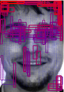
(a) weighted patches

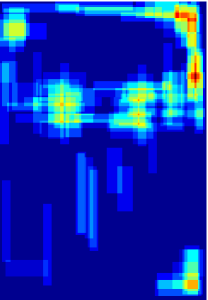
(b) pixel-energy map

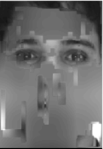
(c) focused face

Figure 1: The demonstration of random face patches. (a): $500$ random face patches with different weights. The weight is represented by the color and width of edges. (b): the corresponding pixel-energy map, the energy of one pixel is defined as the average weight of all the overlapping patches. (c): the simulated focusing behavior. Only a small part of the face is emphasized (focused) while the others are ignored (blurred). The weights are obtained by using the proposed ORE-Learning algorithm on AR [16] dataset.

Compared with the deterministic blocks, random patches have the following two advantages.

• More flexible. The reliable region of a given face could be in arbitrary shape and location. Deterministic blocks are therefore too rudimentary to represent it. The random patch approach, on the other hand, can approximate any shape of interested regions. Figure 1(b) illustrates a pixel-energy map corresponding to the patches shown in Figure 1(a). A pixel’s energy is the mean weights of all the patches covering this pixel. A irregularly-shaped but reasonable region, which includes two eyes and certain parts of the forehead, is emphasized. From a bionic perspective, it is promising to aggregate the random patches for simulating the focusing behavior of human beings. Figure 1(c) illustrates the simulated focusing behavior: the face is blurred according to the pixel-weights, only the focused facial part, a.k.a. the emphasized region, remains clear.

• More efficient. According to Figure 1, only a limited number (always in the order of $10^{1}$ in this work) of patches are taken into consideration. As we empirically proved in the experiment, the complexity of performing the LR method on several small patches are usually lower than that for few large blocks.

3.2 Bayesian Patch Representation

Given that the linear-subspace assumption is more reliable on certain face patches, it is intuitive to perform the LR-method for each patch. In principle, we could employ either member of the LR-family to perform the linear representation on the patches. According to the theoretical analysis [5, 6], however, it seems no need to specifically select a certain subset from ${\mathbf{X}}_{k}$. We thus employ the whole ${\mathbf{X}}_{k}$ to form the representation basis, just like what [4, 5] did. In particular, for class $k$ and patch $t$, we denote the patch set as ${\mathbf{X}}^{t}_{k}=[{\mathbf{x}}^{t}_{1},{\mathbf{x}}^{t}_{2},\cdots,{\mathbf{x}}^{t}_{M}]\in{\mathbb{R}}^{d\times M}$, with each column obtained via vectorizing a image patch. The representation coefficients ${\boldsymbol{\beta}}^{\ast}_{t,k}$, for the $k$th class and $t$th patch is then given by

$${\boldsymbol{\beta}}^{\ast}_{t,k}=({{\mathbf{X}}^{t}_{k}}^{\!\top}{\mathbf{X}}^{t}_{k})^{-1}{{\mathbf{X}}^{t}_{k}}^{\!\top}{\mathbf{y}}.$$ (9)

Then the residual $r_{t,k}$ can be obtained as

$$r_{t,k}=\|{\mathbf{y}}_{t}-{\mathbf{X}}^{t}_{k}{\boldsymbol{\beta}}^{\ast}_{t,k}\|_{2},$$ (10)

where ${\mathbf{y}}_{t}$ is the cropped test image according to the patch location. In this paper, all the patches are normalized so that their $\ell_{2}$ norms are equal to $1$. As a result, $r_{t,k}\in[0,1],~{}\forall t,k$.

Ordinary LR-methods, including the robust variations, only focus on the smallest residual or the corresponding class label. This strategy will lose much useful information. Differing from the conventional manner, we interpret every patch representation as a probability vector ${\mathbf{b}}_{t}$. The $k$th element of ${\mathbf{b}}_{t}$, namely $b_{t,k}$, is the probability that current test patch ${\mathbf{y}}_{t}$ belongs to individual $k$ i.e.

$$b_{t,k}=P\left(\gamma_{\mathbf{y}}=k\mid{\mathbf{y}}_{t}\right).$$ (11)

We obtain the above posteriors by applying the Bayesian theorem. First of all, it is common that all the classes share the same prior probability, i.e. $P\left(\gamma_{\mathbf{y}}=k\right)=1/K,~{}\forall~{}k$. The linear-subspace assumption states that, if one test face belongs to class $k$, the test patch ${\mathbf{y}}_{t}$ should distribute around the linear-subspace spanned by ${\mathbf{X}}^{t}_{k}$. The probability of a remote ${\mathbf{y}}_{t}$ is smaller than the one close to the subspace. In this sense, when the category is known, we can assume the random variable ${\mathbf{y}}_{t}$ belongs to a distribution with the probability density function

$$P\left({\mathbf{y}}_{t}\mid\gamma_{\mathbf{y}}=k\right)=C\cdot\exp(-{r^{2}_{t,k}}/{\delta}),$$ (12)

where $\delta$ is a assumed variance and the $C$ is the normalization factor. This distribution, in essence, is a singular normal distribution as its covariance matrix is singular. Figure 2 depicts the tailored distribution in a $2$-D space for the linear-subspace assumption.

Figure 2: The demonstration of the singular normal distribution tailored to the linear-subspace assumption. The black line indicates the linear-subspace $k$ while different colors represent different probabilities. The surface of the probability density function is also shown above. Note that here $D=2$ thus the subspace can have the dimensionality at most $1$, or in other words, a line.

According to Bayes’ rule, the posterior probability is then derived as

$$\begin{split}b_{t,k}&=\frac{P\left({\mathbf{y}}_{t}\mid\gamma_{\mathbf{y}}=k\right)\cdot P\left(\gamma_{\mathbf{y}}=k\right)}{\sum_{j=1}^{K}P\left({\mathbf{y}}_{t}\mid\gamma_{\mathbf{y}}=j\right)\cdot P\left(\gamma_{\mathbf{y}}=j\right)}\\ &=\frac{C/K\cdot\exp(-r^{2}_{t,k}/\delta)}{\sum_{j=1}^{K}C/K\cdot\exp(-r^{2}_{t,j}/\delta)}\\ &=\frac{\exp(-r^{2}_{t,k}/\delta)}{\sum_{j=1}^{K}\exp(-r^{2}_{t,j}/\delta)}.\end{split}$$ (13)

As an example, Figure 3 shows the distribution of the posterior $b_{t,1}$ when there are only $2$ orthogonal linear-subspaces ($1$ and $2$) and dimensionality $D=2$

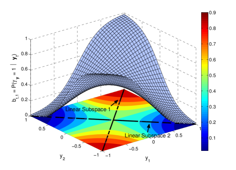
Figure 3: The demonstration of the posterior distribution $b_{t,1}=P\left(\gamma_{\mathbf{y}}=1\mid{\mathbf{y}}_{t}\right)$. The dimensionality of the original space is $2$. In this example, two linear-subspace, i.e. the two black lines, are orthogonal to each other.

We finally aggregate all the posteriors into a vector ${\mathbf{b}}_{t}=[b_{t,1},$ $b_{t,2},$ $\cdots,$ $b_{t,K}]^{{\!\top}}$. The elegant interpretation ${\mathbf{b}}_{t}$, termed Bayesian Patch Representation (BPR), keeps most information related to the representation and thus could lead to a more accurate recognition result. In practice, it makes little sense to impose a constant $\delta$ for all the patches and faces. We thus use normalized one,

$$\delta_{t}=0.1\cdot\min_{k}(r^{2}_{t,k}),$$ (14)

for the $t$th patch.

4 Combine the Bayesian Patch Representations

4.1 Learn a BPR ensemble via Empirical Risk Minimization

Besides the interpretation, the aggregation method is also vital for the final classification. The existing fusion rules, as shown in (8), are rudimentary and non-parameterized thus hard to optimize. In the machine learning community, classifier-ensembles learned via an Empirical Risk Minimization process are considered to be more powerful than the simple methods [17, 18].

As a consequence, we linearly combine the BPRs to generate a predicting vector ${\boldsymbol{\xi}}({\mathbf{y}})$$=$$[\xi_{1}({\mathbf{y}}),\xi_{2}({\mathbf{y}}),$$\dots,$$\xi_{K}({\mathbf{y}})]^{{\!\top}}$$\in{\mathbb{R}}^{K}$, i.e.

$${\boldsymbol{\xi}}({\mathbf{y}})=\sum_{t=1}^{T}\alpha_{t}{\mathbf{b}}_{t}({\mathbf{y}})={\mathbf{B}}({\mathbf{y}}){\boldsymbol{\alpha}},$$ (15)

with $\xi_{k}({\mathbf{y}})$ indicating the confidence that ${\mathbf{y}}$ belongs to the $k$th class, and ${\boldsymbol{\alpha}}=[\alpha_{1},\alpha_{2},\dots,\alpha_{T}]^{{\!\top}}\succcurlyeq\mathbf{0}$. The identity of test face ${\mathbf{y}}$ is then given by

$$\gamma_{\mathbf{y}}=\mathop{\mathrm{argmin}}\limits_{k\in\{1,\cdots,K\}}\xi_{k}({\mathbf{y}})$$ (16)

This kind of linear model dominates the supervised learning literature as it is flexible and feasible to learn. The parameter vector ${\boldsymbol{\alpha}}$ is optimized via minimizing the following Empirical Risk

$${\text{ER}}=\sum_{i}^{N}{\text{Loss}}(z_{i})+\lambda\cdot{\text{Reg}}({\boldsymbol{\alpha}}),$$ (17)

where ${\text{Loss}}(\cdot)$ is a certain loss function, ${\text{Reg}}(\cdot)$ is the regularization term and $\lambda$ is the trade-off parameter. The margin $z_{i}=\mathcal{Z}(l_{i},~{}{\boldsymbol{\xi}}({\mathbf{x}}_{i}))$ reflects the confidence that ${\boldsymbol{\xi}}$ select the correct label for ${\mathbf{x}}_{i}$. Specifically, for binary classifications,

$$z_{i}=\xi_{l_{i}}({\mathbf{x}}_{i})-\xi_{l^{{}^{\prime}}}({\mathbf{x}}_{i}),~{}~{}l^{{}^{\prime}}\neq l_{i}.$$ (18)

For multiple-class problems, however, there is no perfect formulation of $z_{i}$. We then intuitively define the $z_{i}$ as

$$z_{i}=\frac{1}{K-1}\sum_{j\neq l_{i}}^{K}\left(\xi_{l_{i}}({\mathbf{x}}_{i})-\xi_{j}({\mathbf{x}}_{i})\right),$$ (19)

i.e. the mean of all the “bi-class margins”. Recall that $\sum_{j=1}^{K}b_{t,j}({\mathbf{x}}_{i})=1$, we then arrive at a simpler definition of $z_{i}$,

$$z_{i}=\frac{K}{K-1}\sum_{t=1}^{T}\alpha_{t}\left(b_{t,{l_{i}}}({\mathbf{x}}_{i})-\frac{1}{K}\right).$$ (20)

By absorbing the constant $K/(K-1)$ into each $\alpha_{t}$, we have

$$z_{i}=\sum_{t=1}^{T}\alpha_{t}\left(b_{t,{l_{i}}}({\mathbf{x}}_{i})-\frac{1}{K}\right).$$ (21)

The term $b_{t,{l_{i}}}({\mathbf{x}}_{i})-1/K$ can be though of as the confidence gap between using the $t$th BPR and using a random guess. The larger the gap, the more powerful this BPR is. Consequently, $z_{i}$ is the weighted sum of all the gaps, which measures the predicting capability of ${\boldsymbol{\xi}}({\mathbf{x}}_{i})$.

The selection for the loss function and the regularization function has been extensively studied in the machine learning literature [19]. Among all the convex loss formulations, we choose the exponential loss ${\text{Loss}}(z_{i})=\exp(-z_{i})$, motivated by its success in combining weak classifiers[18, 20]. The $\ell_{1}$ norm is adopted as our regularization method since it encourages the sparsity of ${\boldsymbol{\alpha}}$, which is desirable when we want an efficient ensemble. Finally, the optimization problem in this paper is given by:

$$\begin{split}\min_{{\boldsymbol{\alpha}}}~{}&\sum_{i}^{N}\exp\left(-\sum_{t=1}^{T}\alpha_{t}\left(b_{t,{l_{i}}}({\mathbf{x}}_{i})-\frac{1}{K}\right)\right)\\ \mathop{\mathrm{s.t.}}\nolimits~{}&{\boldsymbol{\alpha}}\succcurlyeq\mathbf{0},~{}~{}\|{\boldsymbol{\alpha}}\|_{1}\leq\lambda\end{split}$$ (22)

Note that for easing the optimization, we convert the regularization term to a constraint. With an appropriate $\lambda$, this conversion won’t change the optimization result [21]. The optimization problem is convex and can be solved by using one of the off-the-shelf optimization tools such as Mosek [22] or CVX [23]. The learned model is termed Optimal Representation Ensemble (ORE) as it guarantees the global optimality of ${\boldsymbol{\alpha}}$ from the perspective of Empirical Risk Minimization. The learning algorithm for achieving the ORE is referred to as ORE-Learning.

4.2 Leave-one-out margin

It would be simple to calculate the margin $z_{i}$ if the BPR were model-based, i.e. ${\mathbf{b}}_{t}(\cdot)$ was a set of explicit functions. In fact, that is the situation for most ensemble learning approaches. Unfortunately, that is not the case in this paper where ${\mathbf{b}}_{t}(\cdot)$ is actually instance-based.

For a BPR, we always need a gallery, a.k.a. the representation basis, to calculate ${\mathbf{b}}_{t}(\cdot)$. And ideally, the gallery should be the same for both training and test, otherwise the learned model is only optimal for the training gallery. Nonetheless, we can not directly use the training set, which is the test gallery, as the training gallery. Any training sample ${\mathbf{x}}_{i}$ will be perfectly represented by the whole training set because ${\mathbf{x}}_{i}$ itself is in the basis. Consequently, all BPRs will generate identical outputs and the learned weights $\alpha_{t},~{}\forall t$ will also be the same. To further divide the training set into one basis and one validation set, of course, is a feasible solution. However, it will reduce the classification power of ORE as the larger basis usually implies higher accuracies.

To get around this problem, we employ a leave-one-out strategy to utilize as many training instances as possible for representations. For every training sample ${\mathbf{x}}_{i}$, its gallery is given by

$${\mathbf{x}}_{i}^{C}={\mathbf{X}}\backslash{\mathbf{x}}_{i},$$

i.e. the complement of ${\mathbf{x}}_{i}$ w.r.t. the universe ${\mathbf{X}}$. The leave-${\mathbf{x}}_{i}$-out BPRs, referred to as ${\mathbf{b}}^{{\mathbf{x}}^{C}_{i}}_{t}({\mathbf{x}}_{i}),~{}\forall t$, are yielded based on the gallery ${\mathbf{x}}_{i}^{C}$. The leave-one-out margin $z_{i}$ is then calculated as

$$z_{i}=\sum_{t=1}^{T}\alpha_{t}\left(b^{{\mathbf{x}}_{i}^{C}}_{t,{l_{i}}}({\mathbf{x}}_{i})-\frac{1}{K}\right).$$ (23)

In this way, the size of the training gallery is always $N-1$, we can approximately consider the learned ${\boldsymbol{\alpha}}^{\ast}$ as optimal for the test gallery ${\mathbf{X}}$ with the size of $N$.

After ${\boldsymbol{\alpha}}^{\ast}$ is obtained, we also calculate the leave-one-out predicting vector as

$${\boldsymbol{\xi}}^{{\mathbf{x}}^{C}_{i}}({\mathbf{x}}_{i})={\mathbf{B}}^{{\mathbf{x}}^{C}_{i}}({\mathbf{x}}_{i}){\boldsymbol{\alpha}}^{\ast},$$ (24)

where ${\mathbf{B}}^{{\mathbf{x}}^{C}_{i}}({\mathbf{x}}_{i})$ is the collection of the leave-one-out BPRs. The training error of the ORE-Learning is given by

$$e_{trn}=\frac{1}{N}\sum_{i=1}^{N}\llbracket\mathop{\mathrm{argmax}}\limits_{k}\xi^{{\mathbf{x}}^{C}_{i}}_{k}({\mathbf{x}}_{i})\neq l_{i}\rrbracket,$$ (25)

where $\llbracket\cdot\rrbracket$ denote the boolean operator. This training error, as illustrated below, plays a crucial role in the model-selection procedure of ORE-Learning.

4.3 Training-determined model-selection

Another issue arising here is how to select a proper parameter $\lambda$ for the ORE-Learning. Usually, a validation method such as the $n$-fold cross-validation is performed to select the optimal parameter among candidates. The validation method, however, is expensive in terms of computation, because one needs to repeat the extra “subset training” for $n$ times and usually $n\geq 5$. From the instance-based perspective, a cross-validation is also unacceptable. In every “fold” of a $n$-fold cross-validation, we only use a part of training samples as the gallery. The setting contradicts the principle that one needs to keep the representation basis similar over all the stages.

Fortunately, the leave-one-out margin provides the ORE-Learning an advantage: The training error of the ORE-Learning serves as a good estimate to its leave-one-out error. We can directly use the training error to select the model-parameter $\lambda$. To understand this, let’s firstly recall the definition of the leave-one-out error.

Definition 4.1

(Leave-one-out error [7]) Suppose that ${\mathcal{X}}^{N}$ denotes a training set space comprised of the training sets with $N$ samples $\{{\mathbf{x}}_{1},{\mathbf{x}}_{2},\cdots,{\mathbf{x}}_{N}\}$. Given an algorithm $\mathcal{A}:\bigcup_{N=1}^{\infty}{\mathcal{X}}^{N}\rightarrow\mathcal{F}$, where $\mathcal{F}$ is the functional space of classifiers. The leave-one-out error is defined by

$$e_{loo}\triangleq\frac{1}{N}\sum_{i=1}^{N}\llbracket F^{\mathcal{A}}_{{\mathbf{x}}_{i}^{C}}({\mathbf{x}}_{i})\neq l_{i}\rrbracket,$$ (26)

where $F^{\mathcal{A}}_{{\mathbf{x}}_{i}^{C}}=\mathcal{A}({\mathcal{X}}^{N}\backslash{\mathbf{x}}_{i})$, i.e. the classifier learned using $\mathcal{A}$ based on the set ${\mathcal{X}}^{N}\backslash{\mathbf{x}}_{i}$.

The leave-one-out error is known as an unbiased estimate for the generalization error [7, 24]. Our target in this section is to build the connection between $e_{loo}$ and $e_{trn}$ for ORE-Learning. Suppose that all the training faces are non-disguised, which is the common situation, then let us make the following basic assumption.

Assumption: One patch-location $t$ on the human face could be affected by $Q_{t}$ different expressions. Every expression leads to a distinct and convex Lambertian surface.

According the theory in [5] and [6], the different appearances of one patch surface, caused by illumination changes, span a linear-subspace with a small dimensionality $\Phi$. Given that $M$ training patches from the patch-location $t$ is collected in ${\mathbf{X}}^{t}_{k}$, its arbitrary subset ${\mathbf{X}}^{t}_{P}$ contains $P$ ($P<\Phi\ll M$) samples. With the assumption, we can verify the following lemma.

Lemma 4.1

(The stability of BPRs) If the training subset ${\mathbf{X}}^{t}_{k}$ contains at least $(\Phi Q_{t}+P)$ i.i.d. patch samples, set ${\mathbf{X}}^{t}_{k}$ and set ${\mathbf{X}}^{t}_{k}\backslash{\mathbf{X}}^{t}_{P}$ share the same representation basis.

• Let us denote the linear-subspace formed by ${\mathbf{X}}^{t}_{k}$ as $\mathcal{U}^{t}$. $\mathcal{U}^{t}_{q}$ refers to its subset spanned by the patches associated with surface $q$. We know that

  $${\text{Rank}}(\mathcal{U}^{t})\leq\sum_{q=1}^{Q_{t}}{\text{Rank}}(\mathcal{U}^{t}_{q})=\Phi Q_{t}.$$

  When ${\mathbf{X}}^{t}_{P}$ is moved out, the new linear-subspace spanned by ${\mathbf{X}}^{t}_{k}\backslash{\mathbf{X}}^{t}_{P}$ is denoted by $\tilde{\mathcal{U}}^{t}$. According to the given condition, there are still $\Phi Q_{t}$ i.i.d. patches remaining. Then with an overwhelming probability,

  $${\text{Rank}}(\tilde{\mathcal{U}}^{t})=\Phi Q_{t}={\text{Rank}}(\mathcal{U}^{t}).$$

  Considering that $\tilde{\mathcal{U}}^{t}\subset\mathcal{U}^{t}$, we then arrive at

  $$\tilde{\mathcal{U}}^{t}=\mathcal{U}^{t}.$$

  The space remains the same, so does its basis.  ${\square}$

In contrast, other classifiers, such as decision trees or linear-LDA-classifiers, don’t have this desirable stability. They always depend on the exact data, rather than the extracted space-basis.

Note that $\Phi$ is usually very small [5, 6]. The value of $Q_{t}$ is determined by the types of expressions that can affect patch $t$. It is also very limited if we only consider the common ones. That is to say, with a reasonable number of training samples, the BPRs is stable w.r.t. the data fluctuation. Specifically, when ${\mathbf{x}}_{i}$ is left out ($P=1$), all the BPRs’ values on samples $\{{\mathbf{x}}_{j}\in{\mathbf{X}}\mid j\neq i\}$ won’t change, i.e.

$${\mathbf{b}}^{{\mathbf{x}}^{C}_{j}}_{t}({\mathbf{x}}_{j})={\mathbf{b}}^{{\mathbf{x}}^{C}_{i,j}}_{t}({\mathbf{x}}_{j}),~{}\forall i\neq j,~{}i,j\in\{1,2,\cdots,N\},$$ (27)

where ${\mathbf{x}}^{C}_{i,j}$ stands for the complement of set $\{{\mathbf{x}}_{i},{\mathbf{x}}_{j}\}$. From the perspective of ensemble learning, the original ORE-Learning problem $\mathcal{A}({\mathcal{X}}^{N})$ and the leave-${\mathbf{x}}_{i}$-out problem $\mathcal{A}({\mathcal{X}}^{N}\backslash{\mathbf{x}}_{i})$ share the same “basic hypotheses”

$${\mathbf{b}}_{t}({\mathbf{x}}),~{}\forall t\in\{1,2,\cdots,T\},$$

and constraints

$${\boldsymbol{\alpha}}\succcurlyeq\mathbf{0}~{}\&~{}\|{\boldsymbol{\alpha}}\|_{1}\leq\lambda.$$

The only difference is that the former problem involves one more training sample, ${\mathbf{x}}_{i}$. We know that usually $N\gg 1$, thus one can approximately consider their solutions are the same, i.e.

$${\boldsymbol{\alpha}}^{\ast}_{{\mathbf{x}}_{i}^{C}}={\boldsymbol{\alpha}}^{\ast},~{}~{}\forall i,$$ (28)

where ${\boldsymbol{\alpha}}^{\ast}_{{\mathbf{x}}_{i}^{C}}$ is the optimal solution for problem $\mathcal{A}({\mathcal{X}}^{N}\backslash{\mathbf{x}}_{i})$. Finally, we arrive at the following theorem

Theorem 4.1

With Equation (28) holding, the training error of the ORE-Learning exactly equals to its leave-one-out error.

• In the context of ORE, all types of errors are determined by the predicting vectors ${\boldsymbol{\xi}}({\mathbf{x}}_{i}),~{}\forall i$. For the leave-one-out error, we know that

  $${\boldsymbol{\xi}}^{loo}({\mathbf{x}}_{i})={\mathbf{B}}^{{\mathbf{x}}^{C}_{i}}({\mathbf{x}}_{i}){\boldsymbol{\alpha}}^{\ast}_{{\mathbf{x}}_{i}^{C}}~{}~{}\forall i,$$ (29)

  where ${\mathbf{B}}^{{\mathbf{x}}^{C}_{i}}({\mathbf{x}}_{i})$ is defined in (24). Recall that

  $${\boldsymbol{\xi}}^{trn}({\mathbf{x}}_{i})={\boldsymbol{\xi}}^{{\mathbf{x}}^{C}_{i}}({\mathbf{x}}_{i})={\mathbf{B}}^{{\mathbf{x}}^{C}_{i}}({\mathbf{x}}_{i}){\boldsymbol{\alpha}}^{\ast},~{}~{}\forall i.$$

  If Equation (28) is valid, then obviously, ${\boldsymbol{\xi}}^{trn}({\mathbf{x}}_{i})={\boldsymbol{\xi}}^{loo}({\mathbf{x}}_{i})$. Finally, we have

  $$\begin{split}e_{trn}&=\frac{1}{N}\sum_{i=1}^{N}\llbracket\mathop{\mathrm{argmax}}\limits_{k}\xi^{trn}_{k}({\mathbf{x}}_{i})\neq l_{i}\rrbracket\\ &=\frac{1}{N}\sum_{i=1}^{N}\llbracket\mathop{\mathrm{argmax}}\limits_{k}\xi^{loo}_{k}({\mathbf{x}}_{i})\neq l_{i}\rrbracket\\ &=e_{loo}.\end{split}$$ (30)

  ${\square}$

In practice, Lemma 4.1 and Equation (28) could be only considered as approximately true. However, we still can treat the training error as a good estimate to the leave-one-out error. Recall that $n$-fold cross-validation is an approximation to the leave-one-out validation. Thus the cross-validation error, a commonly used criterion for model-selection, is also a estimate to the leave-one-out error. We then can directly employ the training error of ORE to choose the model-parameter, without an extra validation procedure. The fast model-selection, termed “training-determined model-selection” is justified empirically in the experiment. We tune the $\lambda$ for both ORE and Boosted-ORE, which is introduced below. No significant overfitting is observed.

Corollary 4.1

One can directly set the parameter $\lambda$ to a very small value, e.g. $\lambda=1e$-$5$, to achieve the ORE-model with a good generalization capability.

• Because the training error of a ORE-Learning directly reflects its generalization capability, the ORE-Learning is very resistant to overfittings. Considering that the main reason for imposing the regularization is to curb overfittings, one can totally discard the regularization term in optimization problem (22). However, to prevent the problem from being ill-posed, we still need a constraint for ${\boldsymbol{\alpha}}$. Thus one $\lambda$ with a small value, which implies trivial regularizing effect, is appropriate.  ${\square}$

The above corollary is also verified in the experimental part. Admittedly, without an effective $\ell_{1}$ regularization, one can not expect the obtained ORE-model is sparse and efficient. Consequently, we still conduct the training-determined model-selection to strike the balance between accuracy and efficiency.

5 ORE-Boosting for immense BPR sets

In principle, the convex optimization for the ORE-Learning could be solved perfectly. Nonetheless, sometimes the patch number $T$ is enormous or even nearly infinite. In those scenarios, to solve problem (22) via normal convex solvers is impossible. Recall that boosting-like algorithms can exploit the infinite functional space effectively [17, 18]. We therefore can solve the immense problem in a boosting fashion, i.e. the BPRs are added into the ORE-model one by one, based upon certain criteria.

5.1 Solve the immense optimization problem via the column-generation

The conventional boosting algorithms [17, 18] conduct the optimization in a coordinate-descend manner. However, it is slow and can not guarantee the global-optimality at every step. Recently, several boosting algorithms based on the column-generation [25, 20, 26] were proposed and showed higher training efficiencies. We thus follow their principle to solve our problem.

To achieve the boosting-style ORE-Learning, the dual problem of (22) need to be derived firstly.

Theorem 5.1

The Lagrange dual problem of (22) writes

$$\begin{split}\min_{{\mathbf{u}},r}~{}&r+\frac{1}{\lambda}\sum_{i}^{N}\left(u_{i}\log u_{i}-u_{i}\right)\\ \mathop{\mathrm{s.t.}}\nolimits~{}&\sum_{i=1}^{N}u_{i}\left(b_{t,{l_{i}}}({\mathbf{x}}_{i})-\frac{1}{K}\right)\leq r,~{}~{}\forall t,\\ ~{}&{\mathbf{u}}\succcurlyeq 0.\end{split}$$ (31)

• Firstly, let us rewrite the primal problem (22) as

  $$\begin{split}\min_{{\boldsymbol{\alpha}}}~{}&\sum_{i}^{N}\exp(\varphi_{i})\\ \mathop{\mathrm{s.t.}}\nolimits~{}&\varphi_{i}=-\sum_{t=1}^{T}\alpha_{t}\left(b_{t,{l_{i}}}({\mathbf{x}}_{i})-\frac{1}{K}\right),~{}~{}\forall i,\\ ~{}&{\boldsymbol{\alpha}}\succcurlyeq\mathbf{0},~{}~{}\|{\boldsymbol{\alpha}}\|_{1}\leq\lambda.\end{split}$$ (32)

  After assigning the Lagrange multipliers [21] ${\mathbf{u}}\in{\mathbb{R}}^{N}$, ${\mathbf{q}}\in{\mathbb{R}}^{T}$ and $r\in{\mathbb{R}}$ associated with above constraints, we get the Lagrangian

  where $\theta_{t,i}=b_{t,{l_{i}}}({\mathbf{x}}_{i})-1/K,~{}\forall t,i$ and ${\mathbf{q}}\succcurlyeq\boldsymbol{0}$. The Lagrange dual function is defined as the “infimum” of the Lagrangian, i.e.

  $$\begin{split}\inf_{{\boldsymbol{\alpha}},{\boldsymbol{\varphi}}}L=&\inf_{{\boldsymbol{\varphi}}}\left(\sum_{i=1}^{N}\exp(\varphi_{i})-u_{i}\varphi_{i}\right)-r\lambda\\ &-\overbrace{\left(\sum_{i}^{N}u_{i}{\boldsymbol{\theta}}^{{\!\top}}_{i}+{\mathbf{q}}^{{\!\top}}-r\boldsymbol{1}^{{\!\top}}\right)}^{\text{must be $\boldsymbol{0}$}}{\boldsymbol{\alpha}}\\ =&-\sum_{i=1}^{N}\overbrace{\sup_{\varphi_{i}}(u_{i}\varphi_{i}-\exp(\varphi_{i}))}^{\text{the conjugate of}\exp(\varphi_{i})}-r\lambda\\ =&-\sum_{i=1}^{N}(u_{i}\log u_{i}-u_{i})-r\lambda\end{split}$$ (34)

  where ${\boldsymbol{\theta}}_{i}=[\theta_{1,i},\theta_{2,i},\cdots,\theta_{T,i}]$. After eliminating ${\mathbf{q}}$ we get the first $t$ constraints in the dual problem. The conjugate of function $\exp(\varphi_{i})$ requires that ${\mathbf{u}}\succcurlyeq\boldsymbol{0}$, a.k.a. the second constraint of (31). The dual problem is to maximize the above Lagrangian. After simple algebraic manipulations, (31) is obtained.  ${\square}$

In Theorem 31, ${\mathbf{u}}=[u_{1},u_{2},\cdots,u_{N}]$ is usually viewed as the weighted data distribution. Considering that BPR is instanced-based and thus depends on ${\mathbf{u}}$, we then use ${\mathbf{b}}^{{\mathbf{u}}}_{t}$ to represent the $t$th BPR under the data distribution ${\mathbf{u}}$.

With the column-generation scheme employed in [25, 20, 26] and Theorem 31, we design a boosting-style ORE-Learning algorithm. The algorithm, termed ORE-Boosting, is summarized in Algorithm 1.

Input:

• A set of training data ${\mathbf{X}}=[{\mathbf{x}}_{1},{\mathbf{x}}_{2},\cdots,{\mathbf{x}}_{N}]$.

• A set of patch-locations, indexed by $1,2,\cdots,T$.

• A termination threshold $\epsilon>0$.

• A maximum training step $S$.

• A primitive dual problem:

  $$\min_{{\mathbf{u}},r}~{}r+\frac{1}{\lambda}\sum_{i}^{N}\left(u_{i}\log u_{i}-u_{i}\right),~{}\mathop{\mathrm{s.t.}}\nolimits~{}{\mathbf{u}}\succcurlyeq 0.$$

begin  $\cdot$ Initialize $\boldsymbol{\alpha}=0$, $t=0$, $u_{i}=1/N,~{}\forall i$;

for $s\leftarrow 1$ to $S$ do  $\cdot$ Find a new BPR, ${\mathbf{b}}^{{\mathbf{u}}}_{t^{\ast}}$, such that $$t^{\ast}=\mathop{\mathrm{argmax}}\limits_{t\in\{1,2,\cdots,T\}}\sum_{i=1}^{N}u_{i}\left(b^{{\mathbf{u}}}_{t,{l_{i}}}({\mathbf{x}}_{i})-1/K\right);$$ (35) $\cdot$ if $\sum_{i=1}^{N}u_{i}\left(b^{{\mathbf{u}}}_{t^{\ast},{l_{i}}}({\mathbf{x}}_{i})-1/K\right)<r+\epsilon$, break;

$\cdot$ Assign the inequality

$$\sum_{i=1}^{N}u_{i}\left(b^{{\mathbf{u}}}_{t^{\ast},{l_{i}}}({\mathbf{x}}_{i})-1/K\right)\leq r$$

into the dual problem as its $s$th constraint;

$\cdot$ Solve the updated problem;   $\cdot$ Calculate the primal variable $\boldsymbol{\alpha}$ according to the dual solutions and KKT conditions; end

Output: The Boosted-ORE: ${\boldsymbol{\xi}}({\mathbf{y}})=\mathop{\mathrm{argmax}}\limits_{k}\textstyle\sum_{t=1}^{T}\alpha_{t}\cdot{\mathbf{b}}_{t}({\mathbf{y}})$.

Algorithm 1 ORE-Boosting

5.2 Ultrafast — the data-weight-free training

For the conventional basic hypotheses used in boosting, such as decision trees, decision stumps and the linear-LDA-classifiers, one needs to re-train them after the training samples’ weights ${\mathbf{u}}$ are updated. Usually, the re-training procedure dominates the computational complexity [25, 20].

Apparently, we need to follow this computationally expensive scheme since BPRs are totally data-dependent. It is easy to see the computation complexity of each BPR is

$$C_{L}=\mathcal{O}(M^{3})+\mathcal{O}(M^{2}d),$$ (36)

then the complexity of the training procedure is given by

$$C_{train}=T\cdot S\cdot C_{L}=\mathcal{O}(TSM^{3})+\mathcal{O}(TSM^{2}d),$$ (37)

The whole training procedure could be very slow when $T$ and $S$ are both large.

However, we argue that: the ORE-Boosting can be performed much faster. To explain this, let us firstly rewrite the constraint ${\mathbf{u}}\succcurlyeq\boldsymbol{0}$ in (31) as ${\mathbf{u}}\succ\boldsymbol{0}$. This change won’t influence the interior-point-based optimization method [21]. Then we can prove the following theorem.

Theorem 5.2

Given that ${\mathbf{u}}\succ 0$, The BPRs are independent of the weight vector ${\mathbf{u}}$. In other words, for ORE-Boosting, all the BPRs need to be trained only once.

• let ${\mathbf{U}}_{k}\in\mathbb{R}^{M\times M}$ be the diagonal matrix such that ${\mathbf{U}}_{k}(i,i)={\mathbf{u}}_{k}(i),~{}i=1,2,\dots,M$, where ${\mathbf{u}}_{k}$ is the weight vector for the training face images from the $k$th class. By taking account of the data weight, the representation coefficients associated with patch $t$ are given by.

  $$\hat{{\boldsymbol{\beta}}}^{\ast}_{t,k}=\mathop{\mathrm{argmin}}\limits_{{\boldsymbol{\beta}}}~{}\|{\mathbf{y}}_{t}-{\mathbf{X}}^{t}_{k}{\mathbf{U}}_{k}{\boldsymbol{\beta}}\|_{2},$$ (38)

  which has a closed-form solution that writes

  $$\hat{{\boldsymbol{\beta}}}^{\ast}_{t,k}=({\mathbf{U}}_{k}{{\mathbf{X}}^{t}_{k}}^{{\!\top}}{\mathbf{X}}^{t}_{k}{\mathbf{U}}_{k})^{-1}{\mathbf{U}}_{k}{{\mathbf{X}}^{t}_{k}}^{{\!\top}}{\mathbf{y}}_{t}$$ (39)

  and we know that

  $${\mathbf{u}}\succ 0\implies u_{k}>0\implies{\mathbf{U}}_{k}^{-1}~{}\text{exists.}$$ (40)

  Thus (39) can be further rewritten into

  $$\begin{split}\hat{\boldsymbol{\beta}}^{\ast}_{t,k}&={\mathbf{U}}_{k}^{-1}{({{\mathbf{X}}^{t}_{k}}^{{\!\top}}{\mathbf{X}}^{t}_{k})}^{-1}{\mathbf{U}}_{k}^{-1}{\mathbf{U}}_{k}{{\mathbf{X}}^{t}_{k}}^{{\!\top}}{\mathbf{y}}_{t}\\ &={\mathbf{U}}_{k}^{-1}{({{\mathbf{X}}^{t}_{k}}^{{\!\top}}{\mathbf{X}}^{t}_{k})}^{-1}{{\mathbf{X}}^{t}_{k}}^{{\!\top}}{\mathbf{y}}_{t}\\ &={\mathbf{U}}_{k}^{-1}{\boldsymbol{\beta}}^{\ast}_{t,k},\end{split}$$ (41)

  where ${\boldsymbol{\beta}}^{\ast}_{t,k}$ is the solution to the unweighted BPR. We now can obtain the reconstruction residual $\hat{r}^{t}_{k}$ as

  $$\begin{split}\hat{r}^{t}_{k}&=\|{\mathbf{y}}_{t}-{\mathbf{X}}^{t}_{k}{\mathbf{U}}_{k}\hat{\boldsymbol{\beta}}^{\ast}_{t,k}\|_{2}\\ &=\|{\mathbf{y}}_{t}-{\mathbf{X}}^{t}_{k}{\mathbf{U}}_{k}{\mathbf{U}}_{k}^{-1}{\boldsymbol{\beta}}^{\ast}_{t,k}\|_{2}=r_{t,k}.\\ \end{split}$$ (42)

  This result, without loss of generality, is valid for all the classes and patches. Considering that BPRs are determined by the associated residuals, we arrive at

  $${\mathbf{b}}^{{\mathbf{u}}}_{t,k}={\mathbf{b}}_{t,k}.$$ (43)

  That is to say, training data weights do not have any impact on the BPRs.

  Actually, a more intuitive understanding of the above analysis is in (38): if we treat ${\mathbf{U}}_{k}{\boldsymbol{\beta}}$ as the variable of interest, we solve exactly the same problem as the standard least squares fitting problem.  ${\square}$

According to the theorem, one needs to calculate the BPRs only once. In practice, the following calculations are conducted for all the BPRs and training samples.

$$c^{t}_{i}=b_{t,l_{i}}({\mathbf{x}}_{i})-\frac{1}{K},~{}~{}\forall t,i.$$ (44)

Note that $l_{i}$ is the ground-truth category of ${\mathbf{x}}_{i}$. $T$ oracle vectors ${\mathbf{c}}_{t}=[c^{t}_{1},c^{t}_{2},\cdots,c^{t}_{N}]^{{\!\top}},~{}\forall t$ are stored beforehand. When we performing the ORE-Boosting, the optimization task in (35) is reduced to

$$t^{\ast}=\mathop{\mathrm{argmax}}\limits_{\forall t}\left({\mathbf{c}}_{t}^{{\!\top}}{\mathbf{u}}\right);$$ (45)

With the oracle vectors ${\mathbf{c}}_{t},~{}\forall t$, the training cost is reduced by $S$ times to

$$\tilde{C}_{train}=T\cdot C_{L}=\mathcal{O}(TM^{3})+\mathcal{O}(TM^{2}d).$$ (46)

Usually, $S$ is of order $10^{2}$, so the above strategy can gain a speedup of a few hundred times (see Section 7.6.2). This desirable property makes the proposed ORE-Boosting very compelling in terms of computation efficiency.

6 Face Recognition Using ORE — a Sophisticated Mixture of Inference and Learning

As we discussed above, the LR-based algorithms are generative rather than discriminative. Their main goal is to reconstruct the test face using training faces. From another point of view, every LR-based algorithms is a pure inference procedure using the generative model associated with a specific linear-subspace-assumption. There is no learning process performed because the generative model is predetermined by the theoretical analysis [5, 6]. However, the theoretical proof is only valid under certain ideal conditions and the linear-subspace-assumption itself is an approximation to the derived illumination cone [5]. When this approximated model is applied with “imperfect” gallery faces, accuracy reductions always occur.

The “imperfect” training faces, from another perspective, usually imply more information or patterns involved. By effectively learning the meaningful ones, e.g. expressions and disguises, we can enhance the prior-knowledge-determined model and achieve higher performance. Of course, not all the patterns can be included in the training set. When novel patterns arise during the test, one can only reduce their influence via a inferring process. In this sense, we argue that an ideal face-recognizer should contain two functional parts:

1. A learner, which can extract the existing patterns from the training set.

2. An inference approach, which can recognize the known patterns while discard the foreign ones in the test face.

The learning algorithms for ORE models has been proposed in Section 4 and 5. Now we design the ORE-tailored inference approach.

6.1 Robust-BPR – BPR with a Generic-Face-Confidence

The BPR is informative enough to describe a patch-based LR and one can learn certain face patterns within the ensemble learning framework. However, in the test phase, some unknown patterns, which usually present as non-face patches, might occur. Most LR-methods, including the standard BPR, only pay attention to distinguish the face between different individuals thus can hardly handle this kind of patterns. On the other hand, several evidences [27] suggests that generic faces, including all the categories, also form a linear-subspace. The linear-subspace is sufficiently compact comparing with the general image space. Furthermore, some visual tracking algorithms have already employed LR-approaches (SRC or its variations) to distinguish the foreground from the background [28, 29].

Inspired by the successful implementations, we propose to employ the linear representation for distinguishing face patches from face-unrelated or partly-face patches. Specifically, a badly-contaminated face patch is supposed to be distant from the linear subspace spanned by the training patches in the same position. In this manner, one can measure the degree of contamination for each test patch.

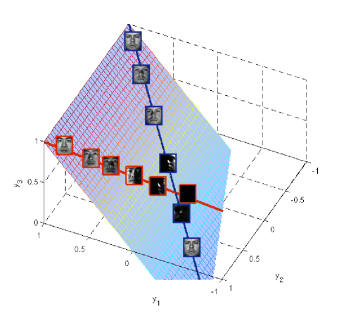
Figure 4: The demonstration of the generic-face subspace in the original $3$-D feature space. Faces from all the categories ($K=2$ here) form a $2$-D linear-subspace, i.e. a plane shown in light blue. Two linear-subspaces, i.e. the lines shown in blue and red respectively, correspond to two different subjects. In this work, however, we are only interested in the face patches and consequently the “generic-face-patch” subspace are considered instead.

Figure 4 illustrates the assumption about the linear-subspace of generic-faces. Note that the faces are merely for demonstration, in this paper, we actually focus on the face patches. According to this assumption, one test patch will be considered as a face part only when it is close enough to the corresponding “generic-face-patch” subspace.

Now we formalize this idea in the Bayesian framework. Given that all the training face patches ${\mathbf{X}}^{t}=[{\mathbf{X}}^{t}_{1},{\mathbf{X}}^{t}_{2},\cdots,{\mathbf{X}}^{t}_{K}]\in{\mathbb{R}}^{d\times N}$ are clean and forming the representation basis, for a test patch ${\mathbf{y}}_{t}$, the reconstruction residual $\tilde{r}^{2}_{t}$ is given by:

$$\tilde{r}^{2}_{t}=\|{\mathbf{y}}_{t}-{\mathbf{X}}^{t}({{\mathbf{X}}^{t}}^{\!\top}{\mathbf{X}}^{t})^{-1}{{\mathbf{X}}^{t}}^{\!\top}{\mathbf{y}}_{t}\|_{2}.$$ (47)

Let us use the notation $u_{t}=1$ to indicate that ${\mathbf{y}}_{t}$ is a face patch while $u_{t}=0$ indicates the opposite. After taking the non-face category into consideration, the original posterior in (11) is equivalent to $P\left(\gamma_{\mathbf{y}}=k~{}|~{}u_{t}=1,{\mathbf{y}}_{t}\right)$. The new target posterior becomes

$$\begin{split}\tilde{b}_{t,k}&=P\left(\gamma_{\mathbf{y}}=k,u_{t}=1\mid{\mathbf{y}}_{t}\right)\\ &=P\left(\gamma_{\mathbf{y}}=k\mid u_{t}=1,{\mathbf{y}}_{t}\right)\cdot P\left(u_{t}=1\mid{\mathbf{y}}_{t}\right)\\ &=b_{t,k}\cdot P\left(u_{t}=1\mid{\mathbf{y}}_{t}\right).\end{split}$$ (48)

Following the principle of linear-subspace, we can assume that

$$\begin{split}P\left({\mathbf{y}}_{t}\mid u_{t}=0\right)&=C_{0}\\ P\left({\mathbf{y}}_{t}\mid u_{t}=1\right)&=C_{1}\cdot\exp(-{{\tilde{r}^{2}_{t}}}/{\tilde{\delta}}),\end{split}$$ (49)

where $C_{1}$, $C_{0}$ is the normalization constant. The subspace for the non-face category is the universe space ${\mathbb{R}}^{d}$, which leads to the uniform distribution $P\left({\mathbf{y}}_{t}\mid u_{t}=0\right)=C_{0}$. Recall that all the patches are normalized, thus the domain of ${\mathbf{y}}_{t}$ is bounded. One can calculate both $C_{1}$ and $C_{0}$ with a specific $\tilde{\delta}$. For simplicity, let us define

$$\tilde{C}=\frac{C_{0}\cdot P\left(u_{t}=0\right)}{C_{1}\cdot P\left(u_{t}=1\right)}=\frac{C_{0}}{C_{1}},$$ (50)

because without any specific prior we usually consider $P\left(u_{t}=0\right)=P\left(u_{t}=1\right)$. We then arrive at the new posterior, which is given by

$$\begin{split}\tilde{b}_{t,k}&=b_{t,k}\cdot P\left(u_{t}=1\mid{\mathbf{y}}_{t}\right)\\ &=\frac{b_{t,k}\cdot P\left({\mathbf{y}}_{t}\mid u_{t}=1\right)\cdot P\left(u_{t}=1\right)}{\sum_{j\in\{0,1\}}P\left({\mathbf{y}}_{t}\mid u_{t}=j\right)\cdot P\left(u_{t}=j\right)}\\ &=\frac{b_{t,k}}{1+\tilde{C}\exp({\tilde{r}^{2}_{t}}/\tilde{\delta})}.\end{split}$$ (51)

In practice, we replace the original $\tilde{b}_{t,k}$ with its upper bound

$$\frac{1}{\tilde{C}}\cdot\exp({-\tilde{r}^{2}_{t}}/\tilde{\delta})\cdot b_{t,k}$$ (52)

Note that the constant $\tilde{C}$ won’t influence the final classification result as all the BPRs are linear combined. As a result, we can discard the term $1/\tilde{C}$ and avoid the complex integral operation for calculating it.

We call the term $\exp(-\tilde{r}^{2}_{t}/\tilde{\delta})$ the Generic-Face-Confidence (GFC) as it peaks when the patch is perfectly represented by generic face patches. With this confidence, we can easily estimate how an image patch is face related, or in other words, how is it contaminated by occlusions or noises. The BPR equipped with a GFC is less sensitive to occlusions and noises, so we refer $\tilde{{\mathbf{b}}}_{t,k}=[\tilde{b}_{t,1},\tilde{b}_{t,2},\cdots,\tilde{b}_{t,K}]$ as the Robust-BPR. The variance $\tilde{\delta}$ is usually data-dependent, we set

$$\tilde{\delta}=0.05\cdot\left(\frac{1}{T}\sum_{t}^{T}\tilde{r}_{t}\right)^{2},$$ (53)

for all the faces.

6.2 The GFC-equipped inference approach

With the unknown patterns, the learned patch-weights $\alpha_{t},~{}\forall t$ could not guarantee their optimality anymore. An highly-weighted patch-location could be corrupted badly on the test image. Consequently, it should merely play a trivial role in the test phase. In other words, the importances of all the patches should be reevaluated. We then employ the proposed GFC to amend the importances for each patch. When the test face is possibly contaminated, we aggregate the Robust-BPRs instead of the original BPRs. In addition, the learned $\alpha_{t},~{}\forall t$ are not as reliable as before thus we replace the original $\alpha_{t}$ with its “faded” version, i.e.

$$\tilde{\alpha}_{t}=\alpha_{t}^{q},~{}~{}q\in[0,1],~{}\forall t,$$ (54)

where $q$ is the “fading coefficient”. The smaller the $q$ is, the less we take account of the learned weights. Now we arrive at the new aggregation, which writes:

$${\boldsymbol{\xi}}=\sum_{t=1}^{T^{\prime}}\alpha_{t}{\mathbf{b}}_{t}~{}\longrightarrow~{}\tilde{{\boldsymbol{\xi}}}=\sum_{t=1}^{T^{\prime}}\alpha_{t}^{q}\text{GFC}_{t}{\mathbf{b}}_{t}$$ (55)

where $T^{\prime}$ is the number of selected patches via the previous ORE-Learning and usually $T^{\prime}\ll T$ as we impose a $\ell_{1}$ regularization on the loss function. Figure 5 gives us a explicit illustration of mechanism of the patch-weight amending procedure. In the upper row, $31$ patches are selected by using ORE-Learning. Their weights are also shown as stems in the left chart. When a test face is badly contaminated by noisy occlusions, as shown in the bottom row, those weights are not reliable anymore. After modified by the proposed methods, all the large weights are assigned to the clean locations. Consequently, the following classification can hardly influenced by the occlusions. From a bionic angle, the weight-amendment is analogue to a focus-changing procedure, as the previously emphasized parts look “unfamiliar” and not reliable anymore.

$\begin{array}[]{lc}\begin{@subfigure}\includegraphics[width=86.72267pt]{select_patches_3_ori}\end{@subfigure}&\begin{@subfigure}\includegraphics[width=238.49231pt]{stem_3_ori}\end{@subfigure}\\ \begin{@subfigure}\includegraphics[width=86.72267pt]{select_patches_3_gfc}\end{@subfigure}&\begin{@subfigure}\includegraphics[width=238.49231pt]{stem_3_gfc}\end{@subfigure}\end{array}$

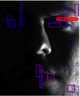
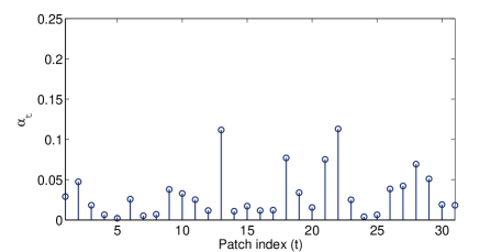
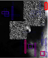
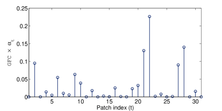
Figure 5: The demonstration for the patch-weight amending method. Upper row: the selected patches by ORE-Learning. Their weights are shown as stems in the left chart. Bottom row: one test face contaminated by three noisy blocks. The patches’ weights are modified by using GFC. We can observe that the ORE model with new weights pay more attention to the clean patches. In other words, the “attention” changes because some pre-trusted parts are not reliable anymore.

The patch-weight amendment and the subsequent aggregation process compose the inference part of the ORE algorithm. To distinguish the inference-facilitated ORE-model from the original ones, we refer to it as Robust-ORE. Compared with the anti-noise method proposed in [3] (see optimization problem (7)), our Robust-ORE does not impose a sparse assumption on the corrupted part thus we can handle much larger occlusions. Furthermore, our method is much faster than the robust SRC while maintains its high robustness, as shown in the experiment. Most recently, Zhou et al. [30] proposed a advanced version of (7) via imposing a spatially-continuous prior to the error vector $e$. The algorithm, admittedly, performed very well, especially on the face with single occlusion. However, we argue that the performance gain is due to the extra spatial prior knowledge. In this paper, none of the spatial relation is considered.

6.3 The learning-inference-mixed strategy

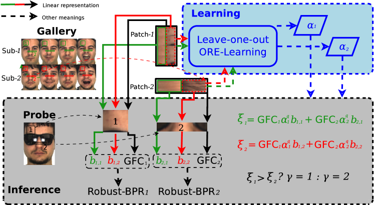
Figure 6: The demonstration of ORE-Learning and the inference procedure. The extremely-simplified problem only contains two subjects and two patch candidates. All the green items are related to Sub-$1$ while the red ones are related to Sub-$2$. The solid arrows indicate linear representation approaches, with different colors standing for different representation basis. The black solid arrows represent the representations based on the all the patches from a certain position while the green and red ones stand for those corresponding to Sub-$1$ and Sub-$2$ respectively.

Figure 6 summarizes the ORE algorithm with a simplified setting where only two subjects (Sub-$1$ and Sub-$2$) and two patches (patch-$1$ on the right forehead and patch-$2$ on the middle face) are involved.

From the flow chart, we can see that the ORE algorithm is, in essence, a sophisticated mixture of inference and learning. First of all, the patches are cropped and collected according to their locations and identities (different columns in one collection). Secondly, the leave-one-out margins are generated based on the leave-one-out BPRs. Then the existing face patterns are learned via the ORE-Learning or ORE-Boosting procedure. The learned results, $\alpha_{1}$ and $\alpha_{2}$, indicate the importances of the two patches. When a probe image is given, one perform $3$ different linear representations for each test patch. The LRs with the patches from Sub-$1$ and Sub-$2$ generate the BPRs $b_{t,1}$ and $b_{t,2}$ ($t\in\{1,2\}$) respectively. In addition, we also use all the patches from one location to represent the corresponding test patch. In this way, the Generic-Face-Confidence (GFC${}_{t},~{}\forall t$) is calculated for each location. When calculating the ORE output $\xi_{i},~{}i\in\{1,2\}$, we multiply the term $\alpha_{t}^{q}b_{t,k}$ with the corresponding GFC_t. In this sense, one reduces the influence of unknown patterns (like the sunglasses in the example) arise in the test image. This is, typically, an inference manner based on the learned information ($\alpha_{1}$ and $\alpha_{2}$) and the prior assumption (the linear-subspaces corresponding to different individuals and the generic face patches). Finally, the identity $\gamma$ is obtained via a simple comparison operation.

The excellence of this learning-inference-mixed strategy is demonstrated in the following experiment part.

7 Experiments

7.1 Experiment setting

We design a series of experiments for evaluating different aspects of the proposed algorithm on two well-known datasets, a.k.a. Yale-B [31] and AR [16]. We compare the recognition rates, between the ORE algorithm and other LR-based state-of-the-arts methods, i.e. Nearest Feature Line (NFL) [1], Sparse Representation Classification (SRC) [3], Linear Regression Classification (LRC) [4] and the two modular heuristics: DEF and Block-SRC. As a benchmark, the Nearest Neighbor (NN) algorithm is also performed. For the conventional LR-based methods, random projection (Randomfaces) [3], PCA (Eigenfaces) [32] and LDA (Fisherfaces) [33] are used to reduce the dimensionality to $25$, $50$, $100$, $200$, $400$. Note that the dimensionality of Fisherfaces are constrained by the number of classes.

The ORE algorithm is performed using the patches each comprised of $225$ pixels. The widths of those patches are randomly selected from the set $\{5,9,15,25,45\}$ and consequently we generate the patches with $5$ different shapes. Random projections are employed to further reduce the dimensionality to $25$, $50$ and $100$. We treat the ORE’s results with original patches ($225$-D) as its $200$-D performance. The inverse value of the trade-off parameter, i.e. $\frac{1}{\lambda}$, is selected from candidates $\{10,20,30,40,50,60,70,80,90,100\}$, via the training-determined model-selection procedure. The variance $\delta$ and $\tilde{\delta}$ are set according to (14) and (53) respectively. We let $q=0.2$ for Robust-ORE. As to ORE-Boosting, we set the convergence precision $\epsilon=1e\text{-}5$ and the maximum iteration number $S=100$.

When carrying out the modular methods, we partition all the faces into $8$ ($4\times 2$) blocks and downsample each block to smaller ones in the size of $12\times 9$, as recommended by the authors [4]. For a fair comparison, we also reduce the dimensionality of the face patches to $100$ using random mapping when performing the ORE algorithm.

We conduct the test in different experimental settings to verify the recognition capacities of our method both in terms of inference and learning. With each experimental setting, the test is repeated $5$ times and we report the average results and the corresponding standard deviations. Every training and test sample, e.g. faces, patches and blocks, are normalized so that

$$\|{\mathbf{x}}_{i}\|_{2}=\|{\mathbf{y}}\|_{2}=1,~{}\forall i.$$

All the algorithms are conducted in Matlab-R2009$a$, on the PC with a $2.6$GHz quad-core CPU and $8$GB RAM. When testing the running speed, we only enable one CPU-core. All the optimization, including the ones for ORE-Learning, ORE-Boosting and SRC, are performed by using Mosek [22].

7.2 Face recognition with illumination changes

Yale-B contains $2,414$ well-aligned face images, belonging to $38$ individuals, captured under various lighting conditions , as illustrated in Figure 7. For each subject, we randomly choose $30$ images to compose the training set and other $30$ images for testing. The Fisherfaces are only generated with dimensionality $25$ as LDA requiring that the reduced dimensionality is smaller than the class number. When performing LRC and ORE with $25$-D data, we only randomly chose $20$ training faces since the least-square-based approaches need an over-determined linear system. For this dataset, we employ $500$ random patches as the task is relatively easy.

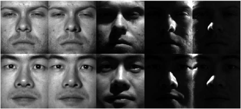
Figure 7: The demonstration of Yale-B dataset with extreme illumination conditions.

		$25$-D	$50$-D	$100$-D	$200$-D	$400$-D
LDA	NN	$93.4\pm 1.3$	-	-	-	-
	NFL	$89.4\pm 1.0$	-	-	-	-
	SRC	$92.5\pm 1.2$	-	-	-	-
	LRC	$58.0\pm 1.9$	-	-	-	-
Rand	NN	$42.6\pm 4.0$	$51.4\pm 1.5$	$54.2\pm 3.0$	$54.8\pm 1.7$	$56.6\pm 1.5$
	NFL	$83.2\pm 1.7$	$88.2\pm 1.0$	$89.5\pm 0.6$	$90.7\pm 0.5$	$90.9\pm 0.4$
	SRC	$80.1\pm 1.6$	$90.7\pm 1.0$	$94.7\pm 0.5$	$96.6\pm 0.7$	$97.1\pm 0.5$
	LRC	$25.9\pm 4.1$	$88.1\pm 0.6$	$93.1\pm 1.2$	$94.5\pm 0.4$	$94.7\pm 0.4$
PCA	NN	$22.3\pm 1.8$	$30.4\pm 1.7$	$34.4\pm 0.5$	$36.6\pm 1.2$	$37.0\pm 1.0$
	NFL	$69.5\pm 1.4$	$77.4\pm 1.2$	$81.4\pm 1.0$	$83.0\pm 0.5$	$83.5\pm 0.5$
	SRC	$80.4\pm 1.6$	$89.1\pm 0.9$	$92.8\pm 0.8$	$94.2\pm 0.7$	$95.1\pm 0.7$
	LRC	$74.7\pm 1.9$	$88.1\pm 0.4$	$89.8\pm 0.3$	$90.7\pm 0.5$	$90.8\pm 0.6$
ORE		$96.5\pm 0.5$	$99.6\pm 0.2$	$99.7\pm 0.1$	$\bf 99.9\pm 0.1$	-
Robust-ORE		$\bf 98.3\pm 0.3$	$\bf 99.8\pm 0.2$	$\bf 99.9\pm 0.1$	$\bf 99.9\pm 0.1$	-
Boosted-ORE		$95.6\pm 1.2$	$99.6\pm 0.2$	$99.8\pm 0.1$	$\bf 99.9\pm 0.1$	-

Table 1: The comparison of accuracy on Yale-B. The highest recognition rates are shown in bold. Note that we only perform algorithms with the Fisherface (LDA) on the $25$-D feature space. The original patch has $225$ pixels, thus we can’t conduct ORE algorithms with $400$-D features.

The experiment results are reported in Table 1. As can be seen, the ORE-based algorithms consistently outperform all the competitors. Moreover, all the proposed methods achieve the accuracy of $99.9\%$ on $200$-D ($225$-D in fact) feature space. To our knowledge, this is the highest recognition rate ever reported for Yale-B under similar circumstances. Given $1,140$ faces are involved as test samples and the recognition rate $99.9\%$, only $1$ faces are incorrectly classified in average. In particular, Robust-ORE, i.e. ORE equipped with Robust-BPRs, shows the highest recognition ability. Its recognition rates are always above $99.8\%$ when $d\geq 50$. The boosting-like variation of the ORE algorithm performs similarly to its prototype and also superior to the performances of other compared methods.

Figure 8 shows the boosting procedure, i.e. the training and test error curves, for the ORE-Boosting algorithm with $100$-D features. We observe fast decreases for both curves. That justifies the efficacy of the proposed boosting approach. Furthermore, no overfitting is illustrated even though the optimal model parameter $\lambda$ is selected according to the training errors. It empirically supports our theoretical analysis in Section 4.3.

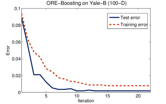
Figure 8: Demonstration of the boosting procedure of ORE-Boosting with $100$-D features on Yale-B.

On Yale-B, both ORE-Learning and its boosting-like cousin only select a very limited part (usually around $5\%$) of all the candidate patches, thanks to the $\ell_{1}$-norm regularization. To illustrate this, Figure 9 shows all the candidates (Figure 9(a)), the selected patches by ORE-Learning (Figure 9(b)), and those selected by ORE-Boosting (Figure 9(c)). We can see that two algorithms make similar selections: in terms of patch positions and patch numbers ($32$ for ORE-Boosting vs. $31$ for ORE-Learning). Nonetheless, minor differences is shown w.r.t. the weight assignment, i.e. assigning values to the coefficients $\alpha_{i},~{}\forall i$. The ORE-Boosting aggressively assigns dominant weights to a few patches. In contrast, ORE-Learning distributes the weights more uniformly. The more conservative strategy often leads to a higher robustness.

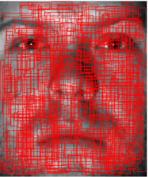
(a) candidates

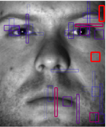
(b) ORE-Learning

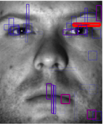
(c) ORE-Boosting

Figure 9: The patch candidates (a) and those selected by ORE-Learning (b) and ORE-Boosting (c). All the patches are shown as blocks. Their widths and colors indicate the associated weights $\alpha_{i},~{}\forall i$. A thicker and redder edge stands for a larger $\alpha_{i}$, i.e. a more important patch. The ORE algorithms are conducted on a $100$-D feature space.

7.3 Face recognition with random occlusions

The above task is completed nearly perfectly. However, sometimes the faces are contaminated by occlusions and most state-of-the-arts may fail on some of them. The most occlusions occur on face images could be divided into two categories: noisy occlusions and disguises. Let us consider the noisy ones first. The noisy occlusions are the ones not supposed to arise on a human face, or in other words, not face-related. They are unpredictable, and thus hard to learn. We then design a experiment to verify the inference capability of ORE-based methods. Considering that ORE-Learning and ORE-Boosting select similar patches, we only perform the former one in this test. To generate the corrupted samples for testing, we impose several Gaussian noise blocks on the Yale-B faces. The blocks are square and in the size of $s\times s,~{}s\in\{20,40,60,80,100,120\}$. The number of the blocks are defined by

$$N_{o}=\text{max}\{\text{round}(0.4\sigma_{f}/s^{2}),3\},$$ (56)

where $\sigma_{f}$ represents the area of the whole face image. That is to say, the occluded parts won’t cover more than $40\%$ area of the original face, unless the number requirement $N_{o}\geq 3$ is not met. The yielded faces are shown in Figure 10. We can see that when $s=120$, the contaminated parts dominate the face image.

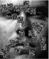
(a) $s=20$

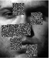
(b) $s=40$

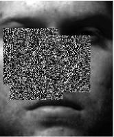
(c) $s=80$

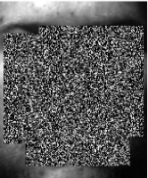
(d) $s=120$

Figure 10: The Yale-B faces with Gaussian noise occlusions. The block size is increased from $20$ to $120$. We can see that when $s=120$, more than $60\%$ of the face image are totally contaminated.

Before testing, we train our ORE models on the clean faces ($30$ faces for each individual). Then, on the contaminated faces (also $30$ faces for each individual), we test the learned models, with or without Robust-BPRs, comparing to the modular heuristics. In this way, we guarantee that no occlusion information is given in the training phase. As a reference, we also perform the standard LRC to illustrate different difficulty levels. The experiment is repeated $5$ times with the training and test faces selected randomly. The results are shown in Table 2.

	$s=20$	$s=40$	$s=60$	$s=80$	$s=100$	$s=120$
LRC ($400$-D)	$74.1\pm 1.4$	$69.7\pm 1.3$	$68.4\pm 1.5$	$45.5\pm 1.4$	$30.4\pm 0.7$	$16.7\pm 0.2$
DEF	$42.9\pm 0.3$	$80.1\pm 0.4$	$88.8\pm 1.0$	$72.3\pm 0.6$	$48.0\pm 1.4$	$26.6\pm 1.3$
Block-SRC	$94.1\pm 0.5$	$93.3\pm 0.5$	$94.1\pm 0.5$	$85.7\pm 0.8$	$78.3\pm 0.4$	$56.8\pm 0.6$
ORE	$93.9\pm 2.6$	$98.2\pm 1.0$	$98.8\pm 0.6$	$97.5\pm 1.7$	$94.2\pm 3.6$	$86.1\pm 8.9$
Robust-ORE	$\bf 98.5\pm 0.7$	$\bf 99.6\pm 0.2$	$\bf 99.7\pm 0.1$	$\bf 99.4\pm 0.5$	$\bf 98.3\pm 1.0$	$\bf 93.8\pm 4.6$

Table 2: The comparison of accuracy on the occluded Yale-B. The highest recognition rates are shown in bold. Robust-ORE represents the ORE-model with Robust-BPRs. Note that the original LRC is performed with $400$-D Randomfaces.

As we can see, again, the proposed ORE models achieve overwhelming performances. In particular, the original ORE-models are nearly (except for the case where $s=20$) consistently better than all the state-of-the-arts. Furthermore, the Robust-ORE models illustrate a very high robustness to the noisy occlusions. It is always ranked first in all the conditions and achieves the recognition rates above $98\%$ when $s<120$. Recall that the performance obtained by ORE models on clean test sets is $99.9\%$. The severe occlusions merely reduce the performance of ORE model by around two percent. When the face is dominated by continuous occlusions ($s=120$), the accuracies of modular methods drop sharply to the ones below $60\%$ while that of Robust-ORE is still above $90\%$. This success justifies our assumption about the generic-face-patch linear-subspace.

7.4 Face recognition with expressions and disguises

Another kind of common occlusions are functional disguises such as sunglasses and scarves. They are, generally speaking, face-related and intentionally put onto the faces. This kind of occlusions are unavoidable in real life. Besides this difficulty, expression is another important influential factor. Expressions invalidate the rigidity of the face surface, which is one foundation of the linear-subspace assumption. To verify the efficacy of our algorithms on the disguises and expressions, we employ the AR dataset. There are $100$ individuals in the AR (cropped version) dataset. Each subject consists of $26$ face images which come with different expressions and considerable disguises such as scarf and sunglasses (see Figure 11).

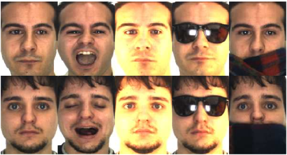
Figure 11: Images with occlusions and expressions in AR dataset. Note that we use only gray-scale faces in the experiment.

First of all, following the conventional scheme, we use all the clean and inexpressive faces ($8$ faces for each individual) as training samples and test the algorithms on those with expressions ($6$ faces per individual), sunglasses ($6$ faces per individual) and scarves ($6$ faces per individual) respectively. Similar to the strategy for handling random occlusions, $500$ random patches are generated and we also employ the Robust-BPRs for testing. The test results can be found in Table 3. Note that the tests for Block-SRC, DEF and LRC are conducted once as the data split is deterministic. Consequently, no standard deviation is reported for those algorithms. The ORE-based methods are still run for $5$ times, with different random patches and random projections.

	Expressions	Sunglasses	Scarves
LRC ($400$-D)	$81.0$	$54.5$	$10.7$
DEF	$88.2$	$91.2$	$85.2$
Block-SRC	$87.5$	$95.7$	$86.0$
ORE	$82.0\pm 1.2$	$85.0\pm 3.9$	$86.5\pm 0.7$
Robust-ORE	$\bf 92.8\pm 0.9$	$\bf 96.1\pm 1.8$	$\bf 95.8\pm 1.2$

Table 3: The comparison of accuracy on the AR dataset. The highest recognition rates are shown in bold. Robust-ORE represents the ORE-model with Robust-BPRs. Note that the original LRC is performed with $400$-D Randomfaces.

According to the table, Robust-ORE beats other methods in all the scenarios. In particular, for the faces with scarves, both of ORE and Robust-ORE are superior to other methods. The performance gap between Robust-ORE and the involved state-of-the-arts is around $10\%$.

7.5 Learn the patterns of disguises and expressions

The expressions and disguises share one desirable property: they can be characterized by typical and limited patterns. One thus can learn those patterns within our ensemble learning framework. To verify the learning power of the proposed method, we re-split the data: for each individual, $13$ images are randomly selected for training while the remaining ones are test images. In this way, the ORE-Learning or ORE-Boosting algorithm is given the information on disguise patterns. The experiment on AR is rerun in the new setting. Table 4 shows the recognition accuracies. Note that the results for the $100$-D Fisherface are actually obtained by using $95$-D features since here ($100$ categories) the dimensionality limit for LDA is $99$.

		$25$-D	$50$-D	$100$-D	$200$-D	$400$-D
LDA	NN	$95.3\pm 0.3$	$97.4\pm 0.6$	$97.9\pm 0.5$	-	-
	NFL	$92.5\pm 0.8$	$96.8\pm 0.4$	$97.9\pm 0.2$	-	-
	SRC	$94.6\pm 0.5$	$97.4\pm 0.5$	$97.9\pm 0.4$	-	-
	LRC	$72.8\pm 1.6$	$94.5\pm 0.4$	$97.1\pm 0.3$	-	-
Rand	NN	$17.0\pm 0.9$	$19.8\pm 1.6$	$22.8\pm 2.3$	$22.2\pm 1.5$	$23.6\pm 1.1$
	NFL	$44.9\pm 3.0$	$55.2\pm 1.9$	$60.9\pm 1.7$	$63.1\pm 1.2$	$65.1\pm 1.2$
	SRC	$45.4\pm 0.5$	$71.3\pm 1.7$	$85.8\pm 1.1$	$91.5\pm 0.7$	$93.9\pm 0.6$
	LRC	$43.0\pm 2.2$	$71.6\pm 1.8$	$78.9\pm 1.3$	$82.1\pm 1.2$	$83.5\pm 0.7$
PCA	NN	$19.4\pm 1.3$	$20.4\pm 1.1$	$21.7\pm 1.3$	$21.8\pm 1.2$	$22.0\pm 1.0$
	NFL	$41.9\pm 1.6$	$48.2\pm 1.2$	$52.1\pm 1.6$	$54.3\pm 1.3$	$55.4\pm 1.3$
	SRC	$52.7\pm 0.8$	$72.1\pm 1.5$	$80.8\pm 1.0$	$83.6\pm 0.5$	$83.9\pm 0.7$
	LRC	$60.3\pm 0.8$	$75.3\pm 1.0$	$80.3\pm 0.7$	$82.1\pm 0.8$	$82.7\pm 0.8$
ORE		$97.0\pm 0.5$	$98.7\pm 0.5$	$99.0\pm 0.3$	$99.1\pm 0.1$	-
Robust-ORE		$\bf 98.4\pm 0.5$	$\bf 99.1\pm 0.4$	$\bf 99.4\pm 0.2$	$\bf 99.5\pm 0.2$	-
Boosted-ORE		$96.8\pm 0.3$	$98.6\pm 0.3$	$98.9\pm 0.3$	$99.0\pm 0.4$	-

Table 4: The comparison of accuracy on AR. The highest recognition rates are shown in bold. Note that we only perform algorithms with the Fisherface (LDA) on the $25$-D and $50$-D feature spaces. The original patch has $225$ pixels, thus we can’t conduct ORE algorithms with $400$-D features.

Similar to the previous test, our methods once again show overwhelming superiority. The Robust-ORE algorithm achieves a recognition rate of $99.5\%$ which is also the best reported result on AR in the similar experimental setting.. In this sense, we can conclude that the ORE algorithms can effectively learn the patterns of disguises. The boosting-like variation of ORE-Learning obtains remarkable performances as well, but is slightly worse than the original version. Besides the ORE algorithms, the Fisherface approach also shows a high learning capacity. With Fisherfaces, the simplest Nearest Neighbor algorithm already achieves the recognition rate of $97.9\%$. This empirical evidence implies that discriminative face recognition methods usually benefit from learning certain face-related patterns.

Figure 12 shows the patch candidates (Figure 12(a)) and the selected ones for ORE-Learning (Figure 12(b)) and ORE-Boosting (Figure 12(c)). As illustrated in the figure, the $500$ patch candidates redundantly samples the face image. Both ORE-Learning and ORE-Boosting choose $54$ patches and ORE-Learning still employs a more conservative strategy of weight assignment. Differing from Figure 9, the ORE algorithms now focus on the forehead more than eyes and the mouth. Considering that sunglasses and scarves are usually located in those two places, the disguises’ patterns are learned and the corresponding patch positions are less trusted during the test.

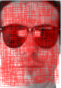
(a) candidates

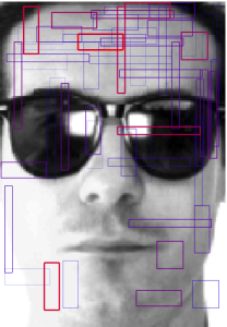
(b) ORE-Learning

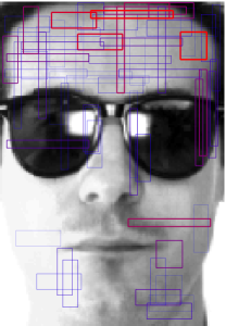
(c) ORE-Boosting

Figure 12: The patch candidates (a) and those selected by ORE-Learning (b) and ORE-Boosting (c). All the patches are shown as blocks. Their widths and colors indicate the associated weights $\alpha_{i},~{}\forall i$. A thicker and redder edge stands for a larger $\alpha_{i}$, i.e. a more important patch. The ORE algorithms are conducted on a $100$-D feature space.

7.6 Efficiency

For a practical computer vision algorithm, the running speed is usually crucial. Here we show the extremely high efficiency of the proposed algorithms, in both terms of training and test.

7.6.1 The verification for the fast model selection

First of all, let us verify the training-determined model-selection for ORE-Learning and ORE-Boosting. Figure 13 demonstrates the training error and test error curves as the model complexity, factorized by $1/\lambda$, is increasing. The two curves, as we can see, show nearly identical tendencies. In particular, when $1/\lambda=1e$-$5$, i.e. only trivial regularization is imposed, we still can not observe any deviation between the two errors. In other words, overfitting does not occur. Consequently, we can employ the training error of ORE-Learning as an accurate measurement of the generalization ability and chose an proper model parameter on it. The required time for model-selection is therefore reduced dramatically.

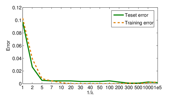
Figure 13: The training errors and test errors change with the increasing model complexity: $\frac{1}{\lambda}$. Note that the $x$-axis is not linearly scaled. The results are generated in a $100$-D feature space with Yale-B faces.

7.6.2 The improvement on the training speed

Besides the fast model selection, we also theoretically validate the fast training procedure. It achieves, as illustrated above, very promising accuracies. Here we evaluate the improvement on the training speed. Figure 14 depicts the difference on the time consumptions for training a Boosted-ORE model, between the methods with and without updating BPRs at every iteration. The test is conducted with the increasing number (from $10$ to $2,000$) of BPRs and trade-off parameter $\lambda=0.02$ in the $100$-D feature space. As illustrated, the efficiency gap is huge. Without the BPR-recalculation, one could save the training time by from $700$ seconds ($10$ BPRs) to more than $10$ days ($2,000$ BPRs).

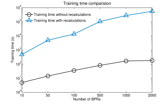
Figure 14: The training times consumed by the ORE-Boosting methods with the BPR recalculations and without them. Note that the $y$-axis is shown in the logarithmic scale. The results are obtained on the AR dataset with $100$-D features.

7.6.3 The highest execution efficiency

At last, let us verify the most important efficiency property — execution speed. The test face (or face patch) is randomly mapped to a lower-dimensional space. Given a reduced dimensionality, all the face recognition algorithms are performed $100$ times on faces from Yale-B. We record the elapsed times (in ms) for each method and show the average values in Figure 15. Note that for LRC and ORE-based methods, there is no need to perform LRs when testing as all the representation bases are deterministic. Before test, one can pre-calculate and store all the matrices

$${\mathbf{E}}=(\hat{{\mathbf{X}}}^{\!\top}\hat{{\mathbf{X}}})^{-1}{\hat{{\mathbf{X}}}}^{\!\top},$$ (57)

where $\hat{{\mathbf{X}}}$ represents different basis for different algorithms. Then the representation coefficients ${\boldsymbol{\beta}}$ for the test face (or patch) ${\mathbf{y}}$ can be obtained via a simple matrix multiplication, i.e.

$${\boldsymbol{\beta}}={\mathbf{E}}{\mathbf{y}}.$$ (58)

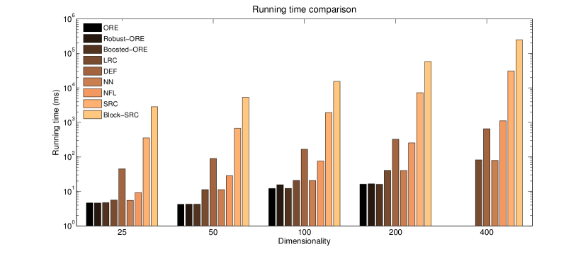
Figure 15: Comparison of the running time. Note that the $y$-axis is in the logarithmic scale. We don’t perform ORE algorithms in the $400$-D feature space as each patch only has $225$ pixels. The $200$-D results for the proposed methods are actually obtained in the original $225$-D space.

As demonstrated, the SRC-based algorithms are the slowest two. The original SRC needs up to $31$ second ($400$-D) to process one test face. The Block-SRC approach, which shows relatively high robustness in the literature, shows even worse efficiency. For $400$-D features, one need to wait more than $4$ minutes for one prediction yielded by Block-SRC. NFL also performs slowly. It requires $9$ to $1,113$ ms to handle one test image. In contrast, the ORE-based methods consistently outperform others in terms of efficiency. In particular, on the $200$-D ($225$-D in fact) feature space, one only needs $16$ ms to identify a probe face by using either ORE algorithm. This speed not only overwhelms those of SRC and NFL, but is also $2$-time higher than those of LRC and NN.

Such a high efficiency, however, seems not reliable. Intuitively, the time consumed by LRC might be always shorter than that for ORE because ORE performs multiple LRs (here actually matrix multiplications) while LRC only performs one. We then track the execution time of the Matlab code via the “profile” facility. We found that, with high-dimensional features and efficient classifiers, it is the dimension reduction which dominates the time usage. The NN and LRC algorithms both perform the linear projection over all the pixels while ORE only select a small part (the pixels in the patches) of them to do the dimension-reduction. As a result, if not too many patches are selected, the ORE algorithms usually illustrate even higher efficiencies than LRC and NN.

Recall that the proposed methods achieve almost all the best recognition rates in different conditions. We draw the conclusion that, the ORE model is a very promising face recognizer which is not only most accurate, but also most efficient.

8 Conclusion and future topics

In this paper, a learning-inference-mixed framework is proposed for face recognition. By observing that, in practice, only partial face is reliable for the linear-subspace assumption. We generate random face patches and conduct LRs on each of them. The patch-based linear representations are interpreted by using the Bayesian theory and linearly aggregated via minimizing the empirical risks. The yielded combination, Optimal Representation Ensemble, shows high capability of learning face-related patterns and outperforms state-of-the-arts on both accuracy and efficiency. With ORE-models, one can almost perfectly recognize the faces in Yale-B (with the accuracy $99.9\%$) and AR (with the accuracy $99.5\%$) dataset, and at a remarkable speed (below $20$ ms per face using the unoptimized Matlab code and one CPU core).

For handling foreign patterns arising in test faces, the Generic-Face-Confidence is derived by taking the non-face patch into consideration. Facilitated by GFCs, the ORE-model shows a high robustness to noisy occlusions, expresses and disguises. It beats the modular heuristics under nearly all the circumstances. In particular, for Gaussian noise blocks, the recognition rate of our method is always above $93\%$ and fluctuates around $99\%$ when the blocks are not too large. For real-life disguises and facial expressions, Robust-ORE also outperforms the competitors consistently.

In addition, to accommodate the instance-based BPRs, an novel ensemble learning algorithm is designed based on the proposed leave-one-out margins. The learning algorithm, ORE-Learning, is theoretically and empirically proved to be resistant to overfittings. This desirable property leads to a training-determined model-selection, which is much faster than conventional $n$-fold cross-validations. For immense BPR sets, we propose the ORE-Boosting algorithm to exploit the vast functional spaces. Furthermore, we also increase the training speed a lot by proving that the ORE-Boosting is actually data-weight-free.

As to the future work, one promising direction is to exploit the spatial information for ORE-models. Similar to [30], one could also employ a Markov Random Field (MRF) method to analyze the patch-based GFCs. Even higher accuracies could be achieved, considering that the GFC is more informative and robust than a single pixel. Secondly, ORE-models can be expanded for the video-based face recognition via using online-learning algorithms. Considering that the Robust-BPRs can distinguish face parts from the non-facial ones, we also want to design a ORE-based face detection algorithm. By merging the detector with this work, we could finally obtain a multiple-task ORE-model that performs the detection and recognition simultaneously.

References

- [1] S.Z. Li and J. Lu, “Face recognition using the nearest feature line method,” IEEE Trans. Neural Netw., vol. 10, pp. 439–443, 1999.
- [2] J. T. Chien and C. C. Wu, “Discriminant waveletfaces and nearest feature classifiers for face recognition,” IEEE Trans. Pattern Anal. Mach. Intell., vol. 24, no. 12, pp. 1644–1649, 2002.
- [3] J. Wright, A.Y. Yang, A. Ganesh, S.S. Sastry, and Y. Ma, “Robust face recognition via sparse representation,” IEEE Trans. Pattern Anal. Mach. Intell., vol. 31, pp. 210–227, 2009.
- [4] N. Imran, T. Roberto, and B. Mohammed, “Linear regression for face recognition.,” IEEE Trans. Pattern Anal. Mach. Intell., vol. 32, no. 11, pp. 2106–12, 2010.
- [5] A.S. Georghiades, P.N. Belhumeur, and D.J. Kriegman, “From few to many: Illumination cone models for face recognition under variable lighting and pose,” IEEE Trans. Pattern Anal. Mach. Intell., vol. 23, no. 6, pp. 643–660, 2001.
- [6] R. Basri and D.W. Jacobs, “Lambertian reflectance and linear subspaces,” IEEE Trans. Pattern Anal. Mach. Intell., pp. 218–233, 2003.
- [7] R. Herbrich, Learning kernel classifiers: theory and algorithms, The MIT Press, 2002.
- [8] X. Wang and X. Tang, “Random sampling LDA for face recognition,” Proc. IEEE Conf. Comp. Vis. Patt. Recogn., 2004.
- [9] N.V. Chawla and K.W. Bowyer, “Random subspaces and subsampling for 2-d face recognition,” in Proc. IEEE Conf. Comp. Vis. Patt. Recogn., 2005, vol. 2, pp. 582–589.
- [10] J. Lu, K.N. Plataniotis, A.N. Venetsanopoulos, and S.Z. Li, “Ensemble-based discriminant learning with boosting for face recognition,” IEEE Trans. Neural Netw., vol. 17, no. 1, pp. 166–178, 2006.
- [11] R. Xiao and X. Tang, “Joint boosting feature selection for robust face recognition,” in Proc. IEEE Conf. Comp. Vis. Patt. Recogn., 2006, vol. 2, pp. 1415–1422.
- [12] X. Wang and X. Tang, “Random sampling for subspace face recognition,” Int. J. Comp. Vis., vol. 70, no. 1, pp. 91–104, 2006.
- [13] Q. Shi, H. Li, and C. Shen, “Rapid face recognition using hashing,” in Proc. IEEE Conf. Comp. Vis. Patt. Recogn., 2010.
- [14] Q. Shi, A. Eriksson, A. van den Hengel, and C. Shen, “Is face recognition really a compressive sensing problem?,” CVPR, 2011.
- [15] P. Viola and M. Jones, “Robust real-time face detection,” Int. J. Comp. Vis., vol. 57, no. 2, pp. 137–154, 2004.
- [16] A.M. Martinez and R. Benavente, “The AR face database,” Tech. Rep., CVC Technical report, 1998.
- [17] R.E. Schapire and Y. Singer, “Improved boosting algorithms using confidence-rated predictions,” Mach. learn., vol. 37, no. 3, pp. 297–336, 1999.
- [18] J. Friedman, T. Hastie, and R. Tibshirani, “Additive logistic regression: A statistical view of boosting,” Ann. Statist., pp. 337–374, 2000.
- [19] T. Hastie, R. Tibshirani, J. Friedman, and J. Franklin, “The elements of statistical learning: data mining, inference and prediction,” Math. Intell., vol. 27, no. 2, pp. 83–85, 2005.
- [20] C. Shen and H. Li, “On the dual formulation of boosting algorithms,” pp. 2216–2231, 2010.
- [21] S. Boyd and L. Vandenberghe, Convex Optimization, Cambridge University Press, 2004.
- [22] A.S. MOSEK, “The mosek optimization software,” Online at http://www. mosek. com, 2010.
- [23] M. Grant and S. Boyd, “Cvx: Matlab software for disciplined convex programming,” Online at http://www.stanford.edu/ boyd/cvx/, 2008.
- [24] T. Evgeniou, M. Pontil, and A. Elisseeff, “Leave one out error, stability, and generalization of voting combinations of classifiers,” Mach. Learn., vol. 55, no. 1, pp. 71–97, 2004.
- [25] A. Demiriz, K.P. Bennett, and J. Shawe-Taylor, “Linear programming boosting via column generation,” Mach. Learn., vol. 46, no. 1-3, pp. 225–254, 2002.
- [26] Z. Hao, C. Shen, N. Barnes, and B. Wang, “Totally-corrective multi-class boosting,” Proc. Asia. Conf. Comp. Vis., pp. 269–280, 2011.
- [27] M. Meytlis and L. Sirovich, “On the dimensionality of face space,” IEEE Trans. Pattern Anal. Mach. Intell., vol. 29, no. 7, pp. 1262–1267, 2007.
- [28] X. Mei and H. Ling, “Robust visual tracking using minimization,” in Proc. IEEE Int. Conf. Comp. Vis., 2009, pp. 1436–1443.
- [29] H. Li, C. Shen, and Q. Shi, “Real-time visual tracking with compressed sensing,” CVPR, 2011.
- [30] Z. Zhou, A. Wagner, H. Mobahi, J. Wright, and Y. Ma, “Face recognition with contiguous occlusion using markov random fields,” in Computer Vision, 2009 IEEE 12th International Conference on. IEEE, 2009, pp. 1050–1057.
- [31] A.S. Georghiades, P.N. Belhumeur, and D.J. Kriegman, “From few to many: Illumination cone models for face recognition under variable lighting and pose,” IEEE Trans. Pattern Anal. Mach. Intell., vol. 23, no. 6, pp. 643–660, 2002.
- [32] M.A. Turk and A.P. Pentland, “Face recognition using eigenfaces,” in Proc. IEEE Conf. Comp. Vis. Patt. Recogn., 1991, pp. 586–591.
- [33] C. Liu and H. Wechsler, “Gabor feature based classification using the enhanced fisher linear discriminant model for face recognition,” IEEE Trans. Image Process., vol. 11, no. 4, pp. 467–476, 2002.