High-field Phase Diagram and Spin Structure of Volborthite Cu₃V₂O₇(OH)${}_{2}\cdot$2H₂O

Abstract

We report results of ⁵¹V NMR experiments on a high-quality powder sample of volborthite Cu₃V₂O₇(OH)${}_{2}\cdot$2H₂O, a spin-1/2 Heisenberg antiferromagnet on a distorted kagome lattice. Following the previous experiments in magnetic fields $B$ below 12 T, the NMR measurements have been extended to higher fields up to 31 T. In addition to the two already known ordered phases (phases I and II), we found a new high-field phase (phase III) above 25 T, at which a second magnetization step has been observed. The transition from the paramagnetic phase to the antiferromagnetic phase III occurs at 26 K, which is much higher than the transition temperatures from the paramagnetic to the lower field phases I ($B$ $<$ 4.5 T) and II (4.5 $<$ $B$ $<$ 25 T). At low temperatures, two types of the V sites are observed with different relaxation rates and line shapes in phase III as well as in phase II. Our results indicate that both phases II and III exhibit a heterogeneous spin state consisting of two spatially alternating Cu spin systems, one of which exhibits anomalous spin fluctuations contrasting with the other showing a conventional static order. The magnetization of the latter system exhibits a sudden increase upon entering into phase III, resulting in the second magnetization step at 26 T. We discuss the possible spin structure in phase III.

1 Introduction

The kagome lattice, a two-dimensional (2D) network of corner-sharing equilateral triangles, is known for strong geometrical frustration. In particular, the ground state of the quantum $S$ = 1/2 Heisenberg model with a nearest-neighbor antiferromagnetic (AF) interaction on the kagome lattice is believed to show no long-range magnetic order. Theories have proposed various ground states such as spin liquids with no broken symmetry with [1] or without [2] a spin-gap or symmetry breaking valence-bond-crystal states [3]. Real materials, however, have secondary interactions, which may stabilize a magnetic order. Effects of the Dzyaloshinsky-Moriya (DM) interaction [4], spatially anisotropic exchange interactions [5, 7, 6], and longer range Heisenberg interactions [8] have been theoretically investigated. In the classical system, it is known that order-by-disorder effect [9] or DM interaction [10] favors long-range order with the $\sqrt{3}\times\sqrt{3}$ pattern or the ${\bf Q}$ = 0 propagation vector, respectively.

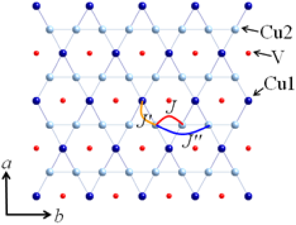
Figure 1: (Color online) Schematic structure of volborthite projected onto the $a$-$b$ plane. The H and O sites are not shown. The V sites are located both below and above the Cu kagome layers. The upper and lower V sites are related by inversion with respect to the Cu sites, hence all V sites are equivalent.

On the experimental side, intensive efforts have been devoted to synthesize materials containing $S$ = 1/2 spins on a kagome lattice [11, 12, 13, 14]. Candidate materials known to date, however, depart from the ideal kagome model in one way or another, such as disorder, structural distortion, anisotropy, or longer range interactions. For example, herbertsmithite ZnCu₃(OH)₆Cl₂ realizes a structurally ideal kagome lattice [12] and exhibits no magnetic order down to 50 mK [15]. However, chemical disorder replacing 10% of Cu²⁺ spins with nonmagnetic Zn²⁺ ions [16] significantly disturbs the intrinsic properties at low temperatures [17, 18].

Volborthite Cu₃V₂O₇(OH)${}_{2}\cdot$2H₂O has distorted kagome layers formed by isosceles triangles. Consequently, it has two inequivalent Cu sites and two kinds of exchange interactions ($J$ and $J^{\prime}$ ) as shown in Fig. 1. The Cu2 sites form linear chains, which are connected through the Cu1 sites. The magnetic susceptibility $\chi$ obeys the Curie-Weiss law $\chi=C/(T+\theta_{W})$ above 200 K with $\theta_{W}$ = 115 K, exhibits a broad maximum at 20 K, and approaches a finite value at the lowest temperatures [11, 19]. An unusual magnetic transition has been observed near 1 K [20, 21, 22, 23], which is much lower than $\theta_{W}$, consistent with strong frustration in a kagome lattice. However, a recent density functional calculation [24] proposed that the frustration is attributed to the competition between a ferromagnetic $J$ and an antiferromagnetic $J^{\prime\prime}$ between second neighbors along the chain (Fig. 1) rather than the geometry of a kagome lattice. Thus the appropriate spin model for volborthite has not been settled yet. Recently, anomalous sequential magnetization steps were reported in a high quality polycrystalline sample at 4.3, 25.5, and 46 T [19]. Furthermore, a magnetization plateau was observed at 2/5 of the saturation magnetization above 60 T [25], in spite of the theoretical prediction for a plateau [26] or a ramp [27] at the 1/3 of the saturation magnetization in an isotropic kagome lattice.

The magnetic transition at $T^{*}\sim 1$ K has been detected by ⁵¹V NMR [21, 22], muon spin relaxation [20], and heat capacity [23] experiments. The NMR measurements revealed a sharp peak in the nuclear relaxation rate 1/$T_{1}$ and broadening of the NMR spectrum due to development of spontaneous moments for the magnetic field $B$ below 4.5 T [22]. A kink was also observed in the heat capacity [23]. Recently, development of short range spin correlation was detected by neutron inelastic scattering experiments [28]. However, the low $T$ phase, which we call phase I, shows various anomalies incompatible with a conventional magnetic order [22]. The NMR line shape is not rectangular but can be fit to a Lorentzian, suggesting a state in which the amplitude of the static moment has spatial modulation, such as a spin density wave (SDW) state or a spatially disordered state. The behavior 1/$T_{1}\propto T$ provides evidence for dense low-energy excitations. The spin-echo decay rate 1/$T_{2}$ is anomalously large, pointing to unusually slow fluctuations.

Above 4.5 T, at which the first magnetization step occurs, another magnetic phase appears with a different spin structure and dynamics [22, 29]. In this phase, which we call phase II, the NMR results show coexistence of two types of the V sites with different values of 1/$T_{2}$ and line shapes [29]. The sites with large 1/$T_{2}$ have similar features to the V sites in phase I. They are strongly coupled to the Cu spins with a spatially modulated structure and large temporal fluctuations. On the other hand, the sites with small 1/$T_{2}$ show a rectangular spectral shape, which is compatible with a conventional order having a fixed magnitude of the ordered moment, such as a Néel state or a spiral order. The numbers of these two sites are nearly equal in a wide range of $B$ and $T$. Based on these observations, a heterogeneous spin state, in which two types of Cu moments form a periodic structure, has been proposed [29].

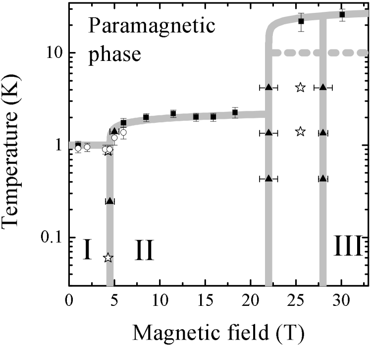
Figure 2: The phase diagram of volborthite proposed from the previous [19, 22] and present studies. The squares (triangles) represent the phase boundaries determined from the variation of the NMR spectra as a function of temperature (magnetic field). The circles and stars indicate the peak of 1/$T_{1}$ [22] and magnetization steps [19], respectively. The lines are guide to the eyes. There is a finite range of field, where phase II and III coexist.

In this paper, we report results of the NMR experiments in higher magnetic fields up to 31 T. The phase diagram determined from the previous [22, 29] and the present experiments is shown in Fig. 2. A new high-field phase defined as phase III is found above 25 T, at which the second magnetization step occurs. The transition from the paramagnetic phase to the phase III takes place at 26 K, which is much higher than the transition temperatures from the paramagnetic to phases I and II. At low temperatures, two types of the V sites are observed in phase III in a similar way as in phase II, indicating that the high-field phase III exhibits also a heterogeneous spin state. Our results show that those Cu spins which are dominantly coupled to the V sites with small 1/$T_{2}$ are responsible for the increase of magnetization at the second step. We propose that the second magnetization step is ascribed to the ferromagnetic alignment of these Cu spins and discuss possible spin structure in phase III, with particular reference to the theories on the anisotropic kagome lattice in the limit $J\gg J^{\prime}$ [6, 5].

2 Experiment

The ⁵¹V NMR measurements have been performed on a high-quality powder sample prepared by the method described in ref. HYoshida. The data at high magnetic fields above 18 T were obtained by using a 20 MW resistive magnet at LNCMI Grenoble. The NMR spectra were recorded at fixed resonance frequency ($\nu_{0}$) by sweeping magnetic field ($B$) in equidistant steps and summing the Fourier transforms of recorded spin-echos, which were obtained by using the pulse sequence $\pi/2-\tau-\pi/2$ [30]. They are plotted against the internal field $B_{\mathrm{int}}=\nu_{0}/\gamma-B$. The NMR spectra are labeled by the reference magnetic field $B_{0}=\nu_{0}/\gamma$. We determined 1/$T_{1}$ by fitting the spin-echo intensity $M(t)$ as a function of the time $t$ after a comb of several saturating pulses to the stretched exponential function $M(t)=M_{eq}-M_{0}\mathrm{exp}\{-(t/T_{1})^{\beta}\}$, where $M_{eq}$ is the intensity at the thermal equilibrium. This functional form was used to quantify the inhomogeneous distribution of $1/T_{1}$. When the relaxation rate is homogeneous, the value of $\beta$ is close to one.

3 Results and Discussion

3.1 Temperature dependence of NMR spectra in high magnetic fields

Figure 3 shows the temperature dependence of the ⁵¹V NMR spectra at $B_{0}$ = 30.1 T. The spectra above 30 K are compatible with a powder pattern due to anisotropic magnetic shifts (inset of Fig. 3). The width due to the quadrupolar interactions is about 0.02 T [22], much smaller than the observed width in this field range. As temperature decreases, the spectral shape begins to change near 26 K. Below 20 K, the spectra show two peaks. Such a structure, which cannot be explained by the anisotropic paramagnetic shift, indicates an internal field due to spontaneous antiferromagnetic (AF) moments. Therefore, our result indicates an AF transition near 26 K at 30 T. Similar measurements at 25.6 T indicate the transition near 22 K. As shown in Fig. 3, the spectral width rapidly increases with decreasing temperature below 15 K. The spectral shape becomes insensitive to the temperature below 4 K, where three broad peaks labeled as $A$, $B$, and $C$ are observed.

Figure 3: (Color online) Temperature dependence of the NMR spectra at $B_{0}$ = 30.1 T. The inset shows an example of calculated powderpattern broadened by a non-axial anisotropic magnetic shift.

The transition temperature of 26 K is much higher than those between the paramagnetic phase and phase I or II below 12 T [22]. Therefore, this suggests a new magnetic phase at high fields which is distinct from phases I and II. Indeed, the magnetization data shows the second step near 26 T, indicating a field-induced magnetic transition. This new high-field phase will be called phase III, as shown in Fig. 2.

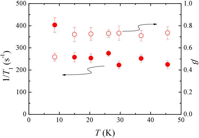
Figure 4: (Color online) Temperature dependences of 1/$T_{1}$ and the strech exponent $\beta$ at 30.1 T.

Figure 4 shows the temperature dependences of 1/$T_{1}$ and the strech exponent $\beta$ at 30.1 T. In the temperature range between 15 and 50 K, 1/$T_{1}$ is independent of temperature. In spite of the clear change in the spectral shape, there is no significant anomaly in 1/$T_{1}$ near 26 K. Let us recall that while the transition from the paramagnetic phase to phase I is marked by a clear peak of 1/$T_{1}$, only a small anomaly in 1/$T_{1}$ was observed at the transition from the paramagnetic phase to phase II [22, 29]. Thus the dynamic signature at the magnetic transition becomes gradually obscured for higher-field phases. However, it is still puzzling that, unlike in phase II, 1/$T_{1}$ no longer decreases below the magnetic ordering temperature in phase III.

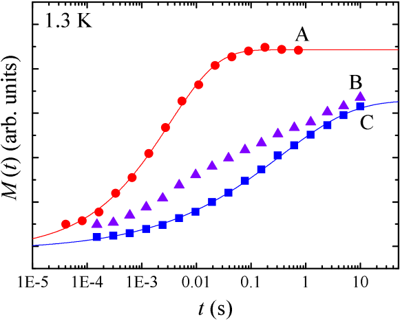
Figure 5: (Color online) Recovery curves $M(t)$ measured at positions $A$, $B$, and $C$ in Fig. 3 at 1.3 K. The solid lines show the fitting to the stretched exponential function $M(t)=M_{eq}-M_{0}\mathrm{exp}\{-(t/T_{1})^{\beta}\}$.

As shown in Fig. 4, $\beta$ decreases with decreasing temperature below 10 K, indicating more inhomogeneous distributions in 1/$T_{1}$. With further decreasing temperature, the distribution of 1/$T_{1}$ becomes too large to determine the representative value of 1/$T_{1}$. In addition, the relaxation rates depend on the spectral position at low temperatures. Figure 5 shows the recovery curves $M(t)$ measured at positions $A$, $B$, and $C$ in Fig. 3 at 1.3 K. The intensity at $A$ is recovered within 0.1 s, while the intensity at $C$ does not saturate even at 10 s. These curves can be fit to the stretched exponential function, and we obtain 1/$T_{1}$ = 311 s^-1 and $\beta$ = 0.49 for $A$ and 1/$T_{1}$ = 2.9 s^-1 and $\beta$ = 0.33 for $C$. The recovery curve at $B$ shows an intermediate behavior between the curves measured at $A$ and $C$. Consequently, $M(t)$ at $B$ does not fit to the stretched exponential function. These results show that the spectra at low temperatures consist at least of two components. This is quite similar to the behavior observed in phase II, where the previous NMR measurements show the coexistence of two components characterized by the large and small values of 1/$T_{2}$ [29]. The two component behavior will be discussed in detail in section 3.3. The onset of rapid spectral broadening (Fig. 3) and the strongly inhomogeneous distribution of 1/$T_{1}$ (Fig. 4) indicate that there may be another transition or crossover at 10 - 15 K. This is shown by the dotted line in Fig. 2.

3.2 Magnetic field dependence of NMR spectra

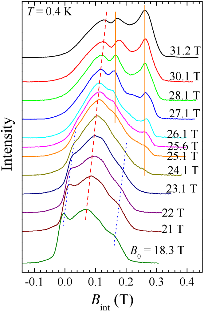
Figure 6: (Color online) Magnetic field dependence of the NMR spectra at 0.4 K. Straight lines are guide to the eye to follow different components (peaks) of the spectra.

Figure 6 shows the field dependence of the ⁵¹V NMR spectra at 0.4 K. The center of gravity of the spectra shifts to larger values of $B_{\mathrm{int}}$ with increasing magnetic field. This shift corresponds to the increase of the magnetization. On the other hand, the width and shape of the spectrum are related to the magnetic structure. As shown in Fig 6, the spectral shapes are almost independent of the magnetic field in the ranges of 18 - 21 T and above 28 T. However, the spectra above 28 T have a different shape from the spectra below 21 T. This indicates that the transition from phase II to phase III occurs in the magnetic field region between 21 and 28 T, and the magnetic structure in phase III is significantly different from that in phase II. In Fig. 6, we observe that the broad peak indicated by the dashed line is present in all the spectra, shifting slightly to higher $B_{\mathrm{int}}$ with increasing magnetic field. In phase II, an additional peak and a shoulder indicated by the dotted lines are observed at lower and higher $B_{\mathrm{int}}$, respectively. They gradually disappears above 22 T. Instead, two additional peaks indicated by the solid lines are observed in phase III. These two peaks gradually develop above 24 T. As the magnetic field increases from 22 to 28 T, there is a gradual transfer of the spectral weight of the peaks denoted by the dotted lines to those denoted by the solid lines, indicating the coexistence of phases II and III.

In order to investigate the phase boundary in more detail, we examine the first and second moments of the spectra defined as,

$$M_{1} = \int B_{\mathrm{int}}I(B_{\mathrm{int}})dB_{\mathrm{int}}$$

$$M_{2} = \int(B_{\mathrm{int}}-M_{1})^{2}I(B_{\mathrm{int}})dB_{\mathrm{int}}$$ (1)

where $I(B_{\mathrm{int}})$ is the NMR spectrum normalized as $\int I(B_{\mathrm{int}})dB_{\mathrm{int}}$ = 1. Figure 7 shows the magnetic field dependence of $M_{1}$. The data below (above) 15 T were taken at 0.3 K (0.4 K). At these sufficiently low temperatures, difference of 0.1 K makes no change in the spectral shape. As shown in Fig. 7, the data below 22 T lie on a straight line through the origin. Above 22 T, $M_{1}$ departs from the straight line. The magnetic field dependence of $M_{1}$ in Fig. 7 reproduces the magnetization curve [19] including the second magnetization step at 26 T.

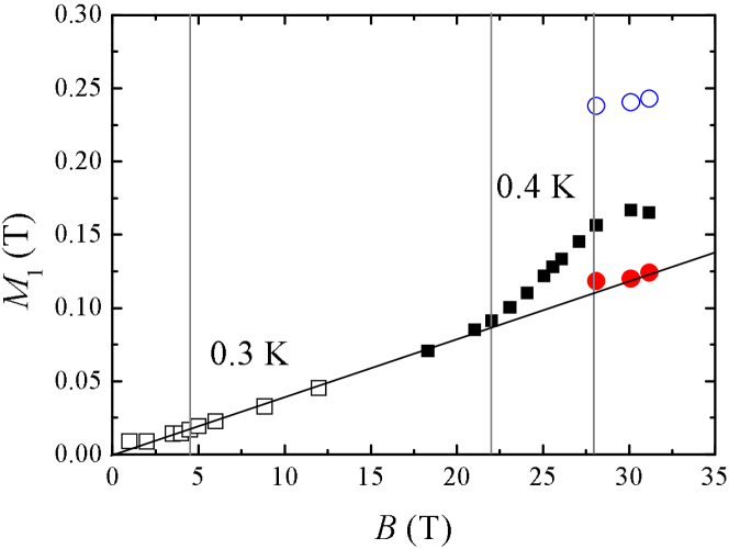
Figure 7: (Color online) Magnetic field dependence of the center of gravity of the spectrum $M_{1}$. The experimental temperature is 0.3 K for the data below 15 T and 0.4 K for the data above 15 T. The open and solid circles represent $M_{1}$ for the slow and fast components, respectively (see the text).

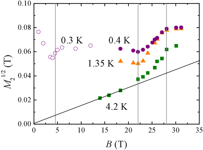
Figure 8: (Color online) Magnetic field dependence of square root of the second moment $M_{2}$. The open and solid circles represent the data at 0.3 and 0.4 K, respectively. The solid triangles and squares represent the data at 1.35 and 4.2 K, respectively.

Figure 8 shows the magnetic field dependence of the line width, i.e. square root of the second moment $M_{2}$, at various temperatures. At 0.3 K, $\sqrt{M_{2}}$ decreases with increasing $B$ below 4.5 T (phase I). For the range of magnetic field 5 - 22 T and at 0.3 - 0.4 K, $\sqrt{M_{2}}$ is almost independent of $B$, indicating that magnetic structure remains unchanged over the entire field range of phase II. Above 28 T, $\sqrt{M_{2}}$ becomes independent of the magnetic field again. Thus the region above 28 T should belong to phase III. For the range of $B$ between 22 and 28 T, $\sqrt{M_{2}}$ increases monotonically with increasing magnetic field. This field region is likely to correspond to the broadened transition due to anisotropy in the powder sample. The similar broadened transition between phases I and II is also observed around 4.5 T with the width of the coexistence region of about 1 T [22]. In both cases, the width of the transition is about 20 - 25% of the center field of the transition. A likely origin of the broadened transition is the anisotropy of $g$ factor, which is estimated to be about 17% from the electron spin resonance measurements [31].

As shown in Fig. 8, $\sqrt{M_{2}}$ at 0.4 and 1.35 K show similar behavior above 18 T, indicating that the transition field is unchanged at these temperatures. On the other hand, $\sqrt{M_{2}}$ at 4.2 K lie on a straight line through the origin below 18 T. This behavior indicates a paramagnetic state, where the internal field is induced by the external magnetic field. However, $\sqrt{M_{2}}$ departs from the straight line above 22 T, indicating the appearance of a spontaneous internal field. Above 28 T, $\sqrt{M_{2}}$ becomes independent of the magnetic field. Therefore, for the field above 28 T, there must be an AF order even at 4.2 K. Thus obtained phase boundaries are plotted by the solid triangles in Fig. 2.

In order to establish the phase boundary between phase II and the paramagnetic phase completely, the temperature dependence of the full width at half maximum (FWHM) of the spectra was measured as shown in Fig. 9 at various magnetic fields. Here, the data below 11.5 T are the same as those presented in ref. MYoshida1. The transition temperatures are determined by the onset of line broadening. Above 8.5 T, the onset is insensitive to the magnetic field as indicated by the arrow in Fig. 9. The transitions observed by our NMR measurements are summarized in Fig. 2. Phases I and II are characterized by a weak field dependences of the transition temperature. Phase III is characterized by much higher transition temperatures compared with phases I and II.

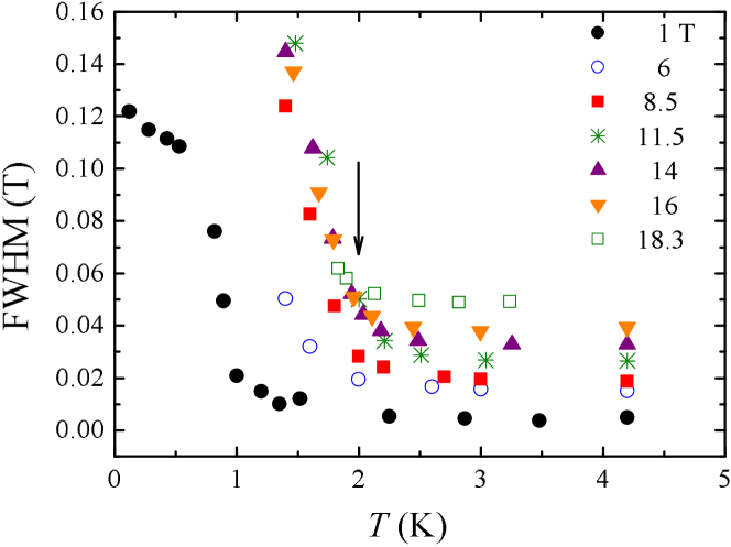
Figure 9: (Color online) Temperature dependences of FWHM at various magnetic fields. The data below 11.5 T are from in ref. MYoshida1.

3.3 Spin structure

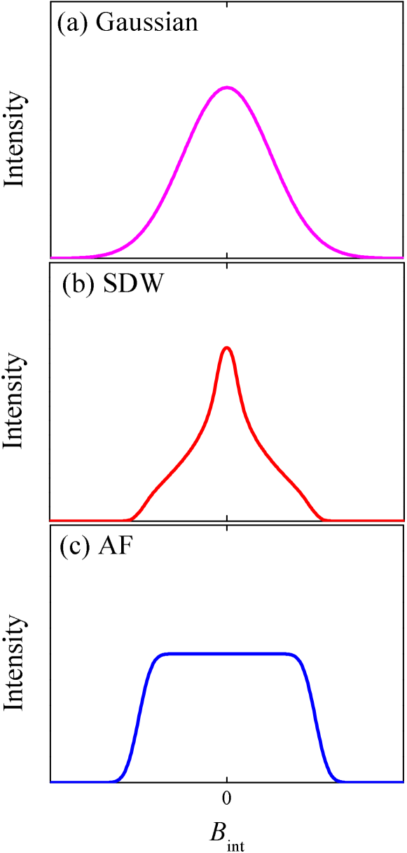
Figure 10: (Color online) Typical powder-pattern spectra for three cases, (a) Gaussian distribution in the magnitude of the internal field , (b) a SDW state where the internal field has a sinusoidal modulation, and (c) an Néel state with a simple two-sublattice structure.

To consider spin structures in the low-temperature phases of volborthite, we begin with general discussion on the powder-pattern NMR spectra for various magnetic states. Figure 10 shows the schematic illustration of the typical powder-pattern for three different antiferromagnetic states. The origin of the horizontal axis is set at the center of gravity of the spectrum. Fig. 10(a) shows a Gaussian spectrum which is expected if the magnitude of the internal field is randomly distributed. Fig. 10(b) shows a spectrum for a spin density wave (SDW) state [32], where the magnitude of the internal field has a sinusoidal modulation. Fig. 10(c) shows a rectangular spectrum, which is expected when the internal field has a fixed magnitude. Examples of this case include a simple Néel state with a two-sublattice structure and a spiral order with an isotropic hyperfine coupling. For both cases (b) and (c), we assume that the direction of the internal field is randomly distributed with respect to the external field, i.e. spin-flop transition does not occur. As shown in Fig. 10, both the SDW and Gaussian distribution give a central peak. They differ only in the way the intensity vanishes on both sides. Since NMR spectra of powder samples are determined by the distribution of the magnitude of $B_{\mathrm{int}}$, it may be difficult to distinguish from the NMR spectra alone between an SDW order, where $B_{\mathrm{int}}$ has a coherent spatial dependence as cos(${\bf Q}\cdot{\bf r}$), and a random distribution of $B_{\mathrm{int}}$, in particular if the distribution is not a Gaussian. On the other hand, it is easy to distinguish those ordered states with spatial modulation in the magnitude of moments such as SDW from the ones with a fixed magnitude of moments. The spectra observed in phase I belongs to the former case as reported in ref. MYoshida1, i.e. the magnitude of the internal field is spatially modulated.

In phase II, the previous NMR results show coexistence of two types of V sites, V_f and V_s sites, which are characterized by the large (fast) and small (slow) relaxation rates, respectively [29]. The spin-echo decay curve in phase II was well fit to the two-component function $I(\tau)=A_{f}\mathrm{exp}(-2\tau/T_{2f})+A_{s}\mathrm{exp}(-2\tau/T_{2s})$. The coefficients $A_{f}$ and $A_{s}$ are proportional to the number of V_f and V_s sites within the frequency window covered by the exciting rf-pulse. Figure 11(a) shows the spectra for the V_f and V_s sites at 6 T and 0.3 K reported in ref. MYoshida2. These spectra are obtained by plotting $A_{f}$ and $A_{s}$ at various frequencies $\nu_{0}$ with the fixed $B$ = 6.0 T, after the two-component fitting has been done. The spectrum of the V_f sites resembles a Gaussian. Therefore, the V_f sites in phase II have a similar feature to the V sites in phase I. These V sites should be surrounded by Cu moments with spatially varying magnitude. On the other hand, the spectrum of the V_s sites shows a rectangular-like shape. indicating that the internal field at the V_s sites is more homogeneous, compared with that at the V_f sites. The spin structure of the V_s sites can be a two-sublattice Néel order or a spiral order with an isotropic hyperfine coupling. When the hyperfine coupling tensor is slightly anisotropic, a spiral order leads to a small modulation of the internal field, resulting in a trapezoidal spectrum. In reality, this may be difficult to distinguish from a rectangular one. Thus we cannot select a unique spin structure.

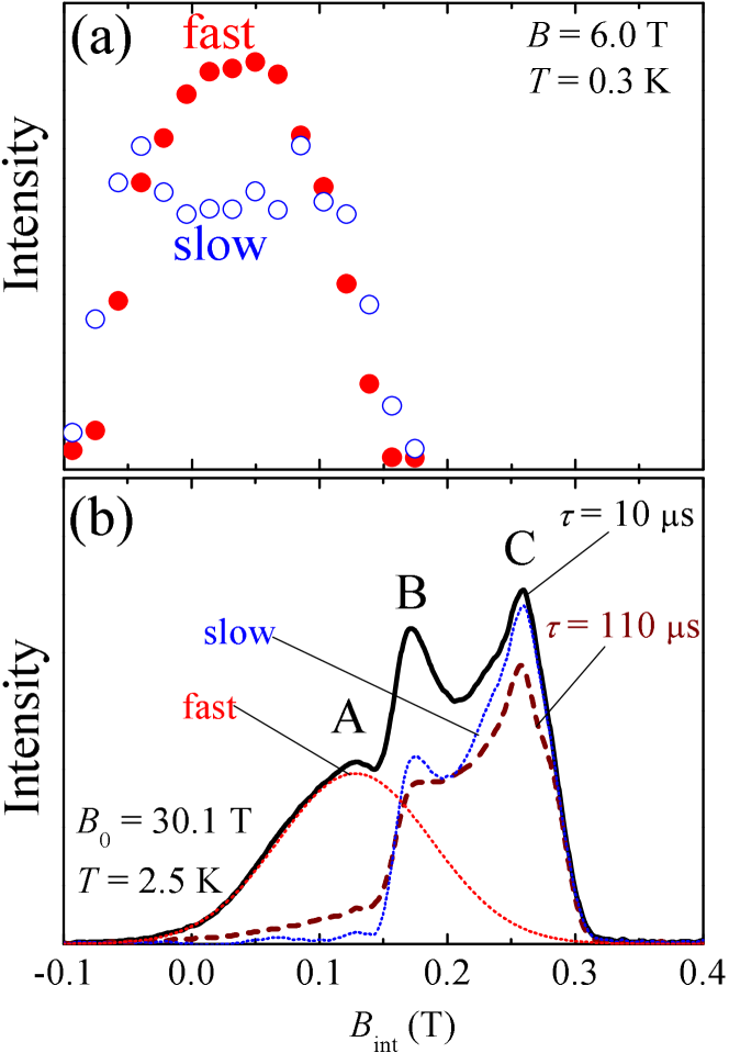
Figure 11: (Color online) (a) NMR spectra for the fast (solid circles) and slow (open circles) components at 0.3 K in the magnetic field of 6.0 T. (b) NMR spectra at $\tau$ = 10 (thick solid line) and 110 $\mu$s (thick dashed line) in the magnetic field of 30.1 T. The red (blue) dotted line represents the NMR spectra for the fast (slow) component.

The multi-component behavior is observed also in phase III by the 1/$T_{1}$ measurements at low temperatures as shown in Fig. 5. These components also exhibit different spin-echo decay rates. In Fig. 11(b), two spectra at 30.1 T and 2.5 K are displayed, one for $\tau$ = 10 $\mu$s and the other for $\tau$ = 110 $\mu$s. The spectrum for $\tau$ = 10 $\mu$s is the same as the one shown in Fig. 3, and the peaks are labeled as $A$, $B$, and $C$. The intensity of the peak $A$ markedly decreases with increasing $\tau$ from 10 to 110 $\mu$s. That is, the $A$ component has large 1/$T_{2}$ as well as large 1/$T_{1}$. The left half of the peak $A$ of the spectrum for $\tau$ = 10 $\mu$s can be fit to a Gaussian labeled as “fast”, which disappears in the spectrum for $\tau$ = 110 $\mu$s. By subtracting the Gaussian component from the spectrum for $\tau$ = 10 $\mu$s, we obtain a rectangular component shown by the dotted line labeled as “slow”. Then, the “slow” component is quite similar to the spectrum for $\tau$ = 110 $\mu$s, indicating that the two-component description is valid also in phase III.

The common feature of phases II and III are two types of V sites, the V_f and V_s sites, of similar characteristics. At the V_f sites, the spectral shapes resembles a Gaussian and the relaxation rates are large. On the other hand, the V_s sites have a rectangular-like spectral shape with relatively small relaxation rates. However, the average values of $B_{\mathrm{int}}$ for the two V sites are quite different for phases II and III as shown in Figs. 11(a) and (b). In going from phase II to phase III, the center of gravity of the whole spectrum shifts to higher values of $B_{\mathrm{int}}$ due to increase of the magnetization. What is more interesting is that the relative positions of the two components change substantially between phases II and III. In phase II, the centers of gravity of the fast and slow components are located almost at the same position, as shown in Fig. 11(a). This shows that the two types of Cu spins, each of which is dominantly coupled to either V_f or V_s sites, have almost the same field-induced averaged magnetization. On the other hand, in phase III, the center of gravity of the slow component is located at a much larger value of $B_{\mathrm{int}}$ than that of the fast component. Therefore, the averaged magnetization coupled to the V_s sites is much larger than that coupled to the V_f sites in phase III. The centers of gravity of the fast and slow components above 28 T are shown in Fig. 7. The former is on the straight line extrapolated from phase II, while the latter is located at much larger $B_{\mathrm{int}}$. Therefore, we conclude that the Cu spins coupled to the V_s sites are responsible for the increase of magnetization at the second step.

The center of gravity $M_{1}$ is related to the magnetization $M$ by the relation $M=M_{1}/A_{\mathrm{hf}}$, where $A_{\mathrm{hf}}$ is the coupling constant determined in the paramagnetic phase $A_{\mathrm{hf}}$ = 0.77 T/$\mu_{B}$ [21, 22]. Indeed, the center of gravity of the whole spectrum at 31 T, $M_{1}$ = 0.165 T, gives the magnetization of 0.21 $\mu_{B}$ in good agreement with the measured magnetization of 0.22 $\mu_{B}$ [19]. By using this relation, the averaged magnetization coupled to the V_f (V_s) sites, $M_{\mathrm{fast}}$ ($M_{\mathrm{slow}}$), at 31 T are estimated to be 0.16 (0.32 $\mu_{B}$). The integrated intensities of the spectra of the fast and slow components are almost the same. This means that numbers of the two sites $N_{f}$ and $N_{s}$ are nearly equal. More precise determination of the ratio $N_{f}:N_{s}$ would require precise knowledge of the frequency dependence of 1/$T_{1}$ and 1/$T_{2}$.

In phase II, a heterogeneous spin state was proposed [29], in which the V_f and V_s sites spatially alternate, because of magnetic superstructure on Cu sites. Arguments were given in ref. MYoshida2 why this is more likely than the macroscopic phase separation. First, the ratio $N_{f}:N_{s}$ should vary as a function of $B$ and $T$, if the V_f and V_s sites belong to distinct phases. Experimentally, however, $N_{f}$ and $N_{s}$ are nearly equal irrespective of $B$ and $T$. Second, the V_f and V_s sites show similar $T$-dependence of 1/$T_{2}$ [29]. This means that the two types of Cu spins coupled to the V_f and V_s sites, respectively, are interacting in a certain way to establish a common $T$-dependence. Again, this is not possible if they belong to different phases.

Although it is difficult to determine the superstructure from the NMR data on a powder sample alone, plausible structures were discussed in the previous paper as follows [29]. The most simple way to generate two types of V sites with the same abundance is to form a superstructure doubling the size of the unit cell. On the ideal kagome lattice, the three directions ${\bf k}_{1}$, ${\bf k}_{2}$, and ${\bf k}_{1}$ + ${\bf k}_{2}$ (Fig. 12 a) are all equivalent. However, in volborthite, the structure is uniform along ${\bf k}_{2}$ and inequivalent Cu1 and Cu2 sites alternate along ${\bf k}_{1}$. Then it is more likely that the superstructure develops along ${\bf k}_{1}$. Consequently, each of the Cu1 and Cu2 sites are divided into two inequivalent sites Cu1_ρ, Cu1_σ and Cu2_κ, Cu2_λ, as shown in Fig. 12(a). It follows that there are two types of the V sites, V_α and V_β, as shown in Fig. 12(a). They should correspond to the V_f and V_s sites. It should be emphasized that distinct spin states on the crystallographically inequivalent Cu1 and Cu2 sites do not account for our observation of two different V sites that are otherwise crystallographically equivalent. Our results can be accounted for only by a symmetry breaking superstructure.

Since a V site is located approximately above or below the center of Cu hexagon of the kagome lattice, the dominant source of the hyperfine field at V nuclei should be confined within the six Cu spins on a hexagon. Because of the distorted structure of volborthite, there are three distinct hyperfine coupling tensors ${\bf A}_{a}$, ${\bf A}_{b}$, and ${\bf A}_{c}$ as shown in Fig. 12(a). The coupling tensors to the other three spins ${\bf A}_{a}^{\prime}$, ${\bf A}_{b}^{\prime}$, and ${\bf A}_{c}^{\prime}$ are generated by the mirror reflection perpendicular to the $b$ axis at the V site. ${\bf A}$ and ${\bf A}^{\prime}$ are the same hyperfine tensors but oriented differently, and they will be effectively different only if the tensor is anisotropic. The coupling constant $A_{\mathrm{hf}}$ determined in the paramagnetic state should be equal to the average of the diagonal components of the sum of these six tensors. The hyperfine fields at the V_α and V_β sites are written as ${\bf B}_{\alpha}=({\bf A}_{a}{\bf s}_{\kappa}+{\bf A}_{a}^{\prime}{\bf s}_{\kappa}^{\prime})+({\bf A}_{b}{\bf s}_{\rho}+{\bf A}_{b}^{\prime}{\bf s}_{\rho}^{\prime})+({\bf A}_{c}{\bf s}_{\lambda}+{\bf A}_{c}^{\prime}{\bf s}_{\lambda}^{\prime})$ and ${\bf B}_{\beta}=({\bf A}_{a}{\bf s}_{\lambda}+{\bf A}_{a}^{\prime}{\bf s}_{\lambda}^{\prime})+({\bf A}_{b}{\bf s}_{\sigma}+{\bf A}_{b}^{\prime}{\bf s}_{\sigma}^{\prime})+({\bf A}_{c}{\bf s}_{\kappa}+{\bf A}_{c}^{\prime}{\bf s}_{\kappa}^{\prime})$, respectively, where ${\bf s}_{\epsilon}$ and ${\bf s}_{\epsilon}^{\prime}$ denote two neighboring spins on the same type of sites (i.e., $\epsilon$ stands for Cu1_ρ, Cu1_σ, Cu2_κ, or Cu2_λ).

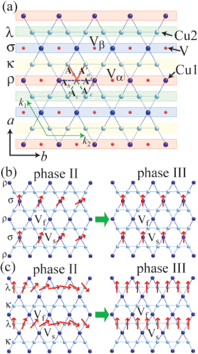
Figure 12: (Color online) Possible magnetic structures in volborthite projected onto the $a$-$b$ plane. (a) Superstructure along the ${\bf k}_{1}$ direction provides two inequivalent V sites, V_α and V_β, and four inequivalent Cu sites, Cu1_ρ, Cu1_σ, Cu2_κ, and Cu2_λ. (b) If the coupling tensors ${\bf A}_{a}$, ${\bf A}_{b}$, and ${\bf A}_{c}$ are largely isotropic and have similar magnitudes, different relaxation behavior at the V_f and V_s sites should be ascribed to the distinct spin states at the Cu1_ρ and Cu1_σ sites. (c) If ${\bf A}_{a}$ is the dominant coupling, different fluctuations at the Cu2_κ and Cu2_λ sites lead to distinction between V_f and V_s.

Both 1/$T_{1}$ and 1/$T_{2}$ are determined by the time correlation function of the hyperfine field [33]. Since the hyperfine coupling to the uniform magnetization $A_{\mathrm{hf}}$ is largely isotropic [22], we expect this is also the case for the individual coupling tensors ${\bf A}_{a}$, ${\bf A}_{b}$, and ${\bf A}_{c}$. If they have similar magnitudes, the coupling to the Cu2 sites is identical for the two V sites, and the different relaxation rates must be ascribed to the difference in the time correlation functions of the Cu1 spins ${\bf s}_{\rho}$ and ${\bf s}_{\sigma}$. The model proposed in ref. MYoshida2 is shown in Fig. 12(b). The Cu1_σ sites develop a long range magnetic order with a uniform magnitude of moments. The spin fluctuations at these sites should have a small amplitude, leading to the slow relaxation at the V_s sites. On the other hand, the Cu1_ρ sites show a modulation in the magnitude of the ordered moments. The absence of fully developed static moments would allow unusually slow fluctuations responsible for the large 1/$T_{2}$ at the V_f sites.

In phase II, the spectra of the V_f and V_s sites have almost the same $M_{1}$, which is proportional to the field. Therefore, all Cu sites have both an AF component and a field-induced uniform component. In phase III, $M_{1}$ is largely shifted only at the V_s sites. This shift can be explained by ferromagnetic alignment of the Cu1_σ sites as shown in the right panel of Fig. 12(b). As shown in Fig. 11, the width of the spectrum of the V_s sites in phase III is narrower than that in phase II. This decrease of the width is also understood by the ferromagnetic saturation of the Cu1_σ sites. Because the ferromagnetic moment is always parallel to the magnetic field, the spectral width is determined by the anisotropy of the hyperfine coupling. Indeed, the spectral shape of the V_s sites in phase III is similar to a paramagnetic powder pattern. In contrast, the width in phase II should be dominantly determined by the AF component. On the other hand, the position and the width of the spectrum of the V_f sites do not change substantially at the transition between phases II and III. This indicates that the Cu1_ρ spins keep spatial modulation of the magnitude of moment in phase III. We should stress that the width of the V_s spectrum is much smaller than the shift $M_{1}$ in phase III, consistent with the largely isotropic hyperfine coupling in the paramagnetic phase [22].

Our results show interesting correspondence with the theory on the anisotropic kagome model in the limit $J\gg J^{\prime}$ [5, 6]. Schnyder, Starykh, and Balents studied the ground state of this model in zero magnetic field. They found that the Cu1 sites develop either a ferromagnetic order or a spiral order with a long wave length with the full moment, while the Cu2 sites have only a small ordered moment [5]. The spin fluctuations at the Cu2 sites associated with the large energy scale $\sim J$ should also lead to a small contributions to 1/$T_{1}$ and 1/$T_{2}$ at the V sites. The irrelevance of the Cu2 sites for both the static internal field and the dynamic relaxation rates at the V sites is consistent with our model that the difference between the V_f and V_s sites are ascribed to the two types of the Cu1 sites. It should be noted, however, that the theory does not account for the superstructure which produces the different V_f and V_s sites.

The similarity between our model shown in Fig. 12(b) and the theoretical prediction on the anisotropic kagome model becomes more apparent in high magnetic fields. A moderate magnetic field should easily drive the small-$Q$ spiral order of the Cu1 sites into a ferromagnetic state. This situation is consistent with our observation of induced ferromagnetism of Cu1_σ spins in phase III. However, our results indicate that only a half of the Cu1 sites undergoes ferromagnetic saturation across the second magnetization step at 26 T. It appears most likely that the other half of the Cu1 sites (the Cu1_ρ sites) get fully polarized across the third step at 46 T. Stoudenmire and Balents investigated the spin structure of the Cu2 sites for the same anisotropic kagome model in high magnetic fields, where Cu1 moments are fully aligned by the field [6]. They found that the Cu2 sites show a quantum phase transition from a ferrimagnetic order along the field direction to an antiferromagnetic order perpendicular to the field with increasing field. A remarkable aspect of the theory is the prediction for a magnetization plateau at 2/5 of the saturation magnetization in the ferrimagnetic region immediately below the transition field.

The 2/5 plateau has been actually observed in the recent magnetization measurements above 60 T [25]. Therefore, we further examine if such a scenario is compatible with our experimental results. When the Cu1 sites exhibit the full moment, $\langle s_{z}\rangle$ = 1/2, in the plateau region, the Cu2 sites should have the averaged moment $\langle s_{z}\rangle$ = 1/20 in order to account for the total magnetization of 2/5 of the saturation. If we assume that all the hyperfine coupling tensors ${\bf A}_{a}$, ${\bf A}_{b}$, and ${\bf A}_{c}$ are isotropic and have the same magnitude, $A_{a}=A_{b}=A_{c}=A_{\mathrm{hf}}$/6 = 0.13 T/$\mu_{B}$, the contribution from the four Cu2 sites to $B_{\mathrm{int}}$ is 0.055 T at all V sites in the plateau region. Here, we used the averaged $g$ value of 2.15.[31, 34] This contribution to $B_{\mathrm{int}}$ will be reduced to 0.028 T at 30 T, assuming that the magnetization at the Cu2 sites is proportional to $B$. In addition, the full moments at the Cu1_σ sites produce $B_{\mathrm{int}}$ = 0.28 T at the V_s sites. The sum of these gives $B_{\mathrm{int}}$ = 0.30 T, which is reasonably close to the observed $M_{1}$ (= 0.24 T) at the V_s sites at 30 T (Fig.  7). On the other hand, $M_{1}$ = 0.12 T at the V_f sites at 30 T corresponds to $\langle s_{z}\rangle$ = 0.17 at the Cu1_ρ sites. The summation of the magnetizations at the Cu2, Cu1_σ, and Cu1_ρ sites amounts to the total magnetization of 0.28 $\mu_{B}$ at 30 T, which is in reasonable agreement with the experimental magnetization of 0.22 $\mu_{B}$. Therefore, this model is semiquantitatively compatible with the NMR and magnetization measurements.

Let us remark that the V_s and V_f sites show extremely different relaxation rates in phase III. As shown in Fig. 5, the V_s sites (line $C$) show two orders of magnitude smaller 1/$T_{1}$ than the V_f sites (line $A$). The spectra in Fig. 11(b) for different values of $\tau$ indicate orders of magnitude difference in 1/$T_{2}$. In contrast, the difference in 1/$T_{2}$ between the V_f and V_s sites is only a factor of four in phase II [29]. In fact the extremely small relaxation rates at the V_s sites in phase III is what should be expected if the moments at the Cu1_σ sites are completely saturated by magnetic fields and the contribution from the Cu2 sites is heavily suppressed for $J\gg J^{\prime}$. On the other hand, in phase II, the spins at the Cu1_σ sites have finite fluctuations even though they show a conventional magnetic order. The anomalous fluctuations of the Cu1_ρ spins can then couple to the fluctuations of the Cu1_σ spins, leading to the similar temperature dependence of 1/$T_{2}$ at the V_f and V_s sites [29].

The above discussion is based on the assumption that all the hyperfine coupling tensors are largely isotropic and have similar magnitudes. However, the low symmetry of the volborthite structure may result in large difference in the hyperfine coupling. In particular, ${\bf A}_{a}$ and ${\bf A}_{c}$ involve significantly different V-O-Cu hybridization paths. If one of them, say ${\bf A}_{a}$, is the dominant coupling, the different relaxation rates for the two V sites must be ascribed to the different dynamics of ${\bf s}_{\lambda}$ and ${\bf s}_{\kappa}$. An example of this case is shown in Fig. 12(c). However, there has been no microscopic theory which supports such a scenario.

4 Summary

We have presented the ⁵¹V NMR results of the $S$ = 1/2 distorted kagome lattice volborthite. Following the previous experiments in magnetic fields below 12 T, the NMR measurements have been extended to higher fields up to 31 T. In addition to the already known two ordered phases (phases I and II), we found a new high-field phase above 25 T, at which the second magnetization step occurs. This high-field phase (phase III) has the transition temperature of about 26 K, which is much higher than those of phase I (1 K) and phase II (1 - 2 K). At low temperatures, two types of the V sites are observed with different relaxation rates and line shapes in phases II and III. Our results indicate that both phases exhibit a heterogeneous spin state, where an ordered state with non-uniform magnitude of moment with anomalous fluctuations alternates with a more conventional order with a fixed magnitude of the ordered moment. The latter group of spins are responsible for the increase of magnetization at the second step between the phase II and phase III. We proposed a possible spin structure in phase III compatible with the NMR and magnetization measurements. Our model has common features with the theories on the anisotropic kagome lattice in the limit $J\gg J^{\prime}$ [5, 6], although the formation of heterogeneous superstructure was not predicted by the theories.

References

- [1] C. Waldtmann, H.-U. Everts, B. Bernu, C. Lhuillier, P. Sindzingre, P. Lecheminant, and L. Pierre: Eur. Phys. J. B 2 (1998) 501.
- [2] M. Hermele, Y. Ran, P. A. Lee, and X.-G. Wen: Phys. Rev. B 77 (2008) 224413.
- [3] R. R. P. Singh and D. A. Huse: Phys. Rev. B 76 (2007) 180407(R).
- [4] O. Cépas, C. M. Fong, P. W. Leung, and C. Lhuillier: Phys. Rev. B 78 (2008) 140405(R).
- [5] A. P. Schnyder, O. A. Starykh, and L. Balents: Phys. Rev. B 78 (2008) 174420.
- [6] E. M. Stoudenmire and L. Balents: Phys. Rev. B 77 (2008) 174414.
- [7] F. Wang, A. Vishwanath, and Y. B. Kim: Phys. Rev. B 76 (2007) 094421.
- [8] J.-C. Domenge, P. Sindzingre, C. Lhuillier, L. Pierre: Phys. Rev. B 72 (2005) 024433.
- [9] J. N. Reimers and A. J. Berlinsky: Phys. Rev. B 48 (1993) 9539.
- [10] M. Elhajal, B. Canals, and C. Lacroix: Phys. Rev. B 66 (2002) 014422.
- [11] Z. Hiroi, M. Hanawa, N. Kobayashi, M. Nohara, H. Takagi, Y. Kato, and M. Takigawa: J. Phys. Soc. Jpn. 70 (2001) 3377.
- [12] M. P. Shores, E. A. Nytko, B. M. Bartlett, and D. G. Nocera: J. Am. Chem. Soc. 127 (2005) 13462.
- [13] Y. Okamoto, H. Yoshida, and Z. Hiroi: J. Phys. Soc. Jpn. 78 (2009) 033701.
- [14] K. Morita, M. Yano, T. Ono, H. Tanaka, K. Fujii, H. Uekusa, Y. Narumi, and K. Kindo: J. Phys. Soc. Jpn. 77 (2008) 043707.
- [15] J. S. Helton, K. Matan, M. P. Shores, E. A. Nytko, B. M. Bartlett, Y. Yoshida, Y. Takano, A. Suslov, Y. Qiu, J.-H. Chung, D. G. Nocera, and Y. S. Lee: Phys. Rev. Lett. 98 (2007) 107204.
- [16] S.-H. Lee, H. Kikuchi, Y. Qiu, B. Lake, Q. Huang, K. Habicht, and K. Kiefer: Nat. Mater. 6 (2007) 853.
- [17] T. Imai, E. A. Nytko, B. M. Bartlett, M. P. Shores, and D. G. Nocera: Phys. Rev. Lett. 100 (2008) 077203.
- [18] A. Olariu, P. Mendels, F. Bert, F. Duc, J. C. Trombe, M. A. de Vries, and A. Harrison: Phys. Rev. Lett. 100 (2008) 087202.
- [19] H. Yoshida, Y. Okamoto, T. Tayama, T. Sakakibara, M. Tokunaga, A. Matsuo, Y. Narumi, K. Kindo, M. Yoshida, M. Takigawa, and Z. Hiroi: J. Phys. Soc. Jpn. 78 (2009) 043704.
- [20] A. Fukaya, Y. Fudamoto, I. M. Gat, T. Ito, M. I. Larkin, A. T. Savici, Y. J. Uemura, P. P. Kyriakou, G. M. Luke, M. T. Rovers, K. M. Kojima, A. Keren, M. Hanawa, and Z. Hiroi: Phys. Rev. Lett. 91 (2003) 207603.
- [21] F. Bert, D. Bono, P. Mendels, F. Ladieu, F. Duc, J.-C. Trombe, and P. Millet: Phys. Rev. Lett. 95 (2005) 087203.
- [22] M. Yoshida, M. Takigawa, H. Yoshida, Y. Okamoto, and Z. Hiroi: Phys. Rev. Lett. 103 (2009) 077207.
- [23] S. Yamashita, T. Moriura, Y. Nakazawa, H. Yoshida, Y. Okamoto, and Z. Hiroi: J. Phys. Soc. Jpn. 79 (2010) 083710.
- [24] O. Janson, J. Richter, P. Sindzingre, and H. Rosner: Phys. Rev. B 82 (2010) 104434.
- [25] Y. Okamoto, M. Tokunaga, H. Yoshida, A. Matsuo, K. Kindo, and Z. Hiroi: Phys. Rev. B 83 (2011) 180407(R).
- [26] K. Hida: J. Phys. Soc. Jpn. 70 (2001) 3673.
- [27] H. Nakano and T. Sakai: J. Phys. Soc. Jpn. 79 (2010) 053707.
- [28] G. J. Nilsen, F. C. Coomer, M. A. de Vries, J. R. Stewart, P. P. Deen, A. Harrison, H. M. Ronnow: arXiv:1001.2462v2.
- [29] M. Yoshida, M. Takigawa, H. Yoshida, Y. Okamoto, and Z. Hiroi: Phys. Rev B 84 (2011) 020410(R).
- [30] W. G. Clark, M. E. Hanson, F. Lefloch, and P. Ségransan: Rev. Sci. Instrum. 66 (1995) 2446.
- [31] H. Ohta, W.-M. Zhang, S. Okubo, M. Tomoo, M. Fujisawa, H. Yoshida, Y. Okamoto, Z. Hiroi: J. Phys.: Conf. Series 145 (2009) 012010.
- [32] M. Kontani, T. Hioki, and Y. Masuda: J. Phys. Soc. Jpn. 39 (1975) 672.
- [33] C. P. Slichter, Principles of Magnetic Resonance (Springer, Heidelberg, 1990).
- [34] W.-M. Zhang: Ph.D. thesis, Kobe University, 2010.