Multipartite nonlocality swapping

Abstract

Nonlocality swapping of bipartite binary correlated boxes can be realized by a coupler ($\chi$) in nonsignaling models. By studying the swapping process we find that the previous bipartite coupler can be applied to the swapping of two multipartite boxes, and then generate a multipartite box with more users than that of any of the boxes before swapping. Here quantum bound still appears in the scheme. The bipartite coupler also can be applied to a hybrid scheme of generating a multipartite extremal box from many PR boxes. As the analogue of multipartite entanglement swapping, we generalize the nonlocality swapping of bipartite binary boxes to multipartite binary boxes by using a multipartite coupler $\chi_{N}$, and get the probability of success by connecting the coupler to the generalized Svetlichny inequality. The multipartite coupler acting on many multipartite boxes makes multipartite nonlocality swapping be a more efficient device to manipulate nonlocality between many users. The results show that Tsirelson’s bound for quantum nonlocality emerges only when two of the $n$ boxes involved in the coupler process are noisy ones.

I introduction

Violation of local realism is a fascinating phenomenon of quantum mechanics (QM). Since the paradox was presented by Einstein, Podolsky and RosenEPR in 1935, QM was at one time under suspicion until BellBell showed that there existed certain settings for physical experiments that contradicted ’common sense’ views of reality. Bell’s theorem was proved by the experimentAspect in 1982 and other more later. Nowadays, quantum nonlocality is getting the attention it deserves as another special aspect of the quantum correlations-entanglement.

To get more insight of quantum mechanics, it makes sense to have a study on the connection between quantum entanglement and quantum nonlocality. Like Von Neumann entropy and concurrenceWootters for entanglement, various criteria were put forward to give a convenient test of nonlocality. The earliest one-Bell inequalityBell which comes from Bell’s theorem gives a criterion that classic local correlation must obey. Numbers of Bell-type inequalitiesCHSH ; CH ; Sv were presented for different systems afterwards. The violation of Bell-type inequality gives a straightforward impression about quantum nonlocal correlations (QNC). A common feature for all these inequalities is that QM’s violation can’t reach the maximum value. Naturally, Popescu and RohrlichPR showed a correlation gives a maximal violation 4 of Clauser-Horne-Shimony-Holt (CHSH) inequalityCHSH , while the maximal violation in QM domain, i.e. Tsirelson’s boundbound $\mathcal{B}_{\mathcal{Q}}=2\sqrt{2}$ by QNC. Similarly, an algebraic maximum 8resource and quantum bound $4\sqrt{2}$ by Svetlichny inequalitySv exist in tripartite system. With the addition of the correlations over quantum bound, postquantum correlations (PQC), nonlocal correlations were discussed in generalized nonsignaling models, as nonsignaling correlated boxesresource decided by joint probability distributionnonsign . Strong information-theoretic capabilities were revealed in the study of PQCpost , such as secure cryptographysecure and the reduction of communication complexityNLDC ; complexit .

Properties of entanglement, such as monogamy, distillation, and swapping, were proved to be capable for nonlocality in nonsignaling theorynonsign ; NLD ; NLS , but distinctions still exist between entanglement and nonlocality. Local operations and classic communication (LOCC) were essential in entanglement distillation processes, but nonlocality distillation occurs without CCNLD . Only the operations on the input and output of nonlocal boxes are crucial to the distillation of nonlocality. Dramatically, the device operating on the outside of the boxes failed to swap the correlation between nonlocal boxesNLfS . Skrzypczyk et al.NLD raised the concept of genuine boxes and coupler as analogue of the quantum joint measurement for nonlocality swapping. Clauser-Horne (CH) inequalityCH as an appropriate measure of nonlocality was applied to obtain the possibility of successful swapping. The fact that only PQC can be successfully swapped in isotropic resources makes the emergence of Tsirelson’s bound under CH expression. Then, Skrzypczyk and Brunnercoupler considered all theoretically possible couplers, ranging from perfect to minimal couplers, for limited nonlocality, and quantum bound still appeared in their study.

Zukowski et al.ES proposed the first entanglement swapping scheme, and it was soon generalized to the case of generating a three-particle Greenberger-Horne-Zeilinger (GHZ) state from three Bell pairstriES . Bose et al.multiES generalized the procedure of entanglement swapping to the multiparticle case. A natural question whether multipartite nonlocal correlations can be swapped raises to us. Exploring the analog of multiparticle entanglement swapping, we’ll try to design a generalized multipartite coupler for realizing multipartite nonlocality swapping.

Replacing the CH inequality by CHSH inequalityCHSH and the generalized Svetlichny inequalityGSI , we find that the existing bipartite coupler provides an adequate dynamical process for two correlated nonlocal boxes, including multipartite ones. But this bipartite-coupler-based swapping consumes much resources and seems less efficient in the case of swapping of multi nonlocal boxes. Then we will show a generalized coupler, which can be applied on many multipartite boxes, makes the swapping of many multipartite boxes succeed in a more efficient way.

The paper is organized as follows. In Sec.II we briefly review the quantum nonlocality swapping of two bipartite binary correlated boxes and show the key points therein. In Sec.III, we define the general multipartite binary correlated boxes after presenting the form of the generalized Svetlichny inequality for nonsignal systems. In Sec.IV we generalize the nonlocality swapping on two bipartite boxes to the case of two multipartite boxes by using the bipartite coupler $\chi$ and give a discussion on the bound of quantum nonlocal correlation. In Sec.V we attempt to achieve the nonlocality swapping on three bipartite boxes and then we show the multipartite coupler $\chi_{N}$ for nonlocality swapping on arbitrary number of multipartite boxes. Conclusions and remarks are presented in Sec.VI.

II Framework

Firstly, we’ll give a brief review on Skrzypczyk’s nonlocality swapping schemeNLS . Bob shares two nonlocal boxes with another two spatially separated users Alice and Charlie (See FIG.1).

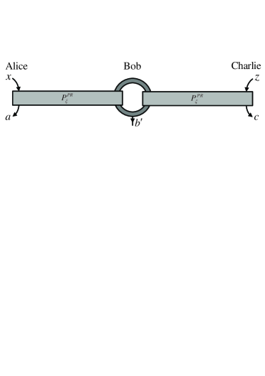
Figure 1: Nonlocality swapping of two isotropic boxes. The coupler is the analogue of quantum joint measurement, and quantum bound (Tsirelson’s bound) emerges in this process.

Bob carries out the bipartite coupler $\chi$ on two bipartite isotropic boxes $P^{\text{PR}}_{\xi}(ab_{1}|xy_{1})$ and $P^{\text{PR}}_{\xi}(b_{2}c|y_{2}z)$, which are superposition of Popescu-Rohrlich (PR) boxresource and the fully mixed box $\openone$NLDC .

$$P^{\text{PR}}_{\xi}={\xi}P^{\text{PR}}+(1-\xi)\openone.$$ (1)

Where $\xi\in[-1,1]$, and when $\xi=-1$, the box is ’anti-PR’ box $P^{\overline{\text{PR}}}$ given by $a\oplus b=xy\oplus 1$.

The output $b^{\prime}=0$ indicates that the correlation between Alice and Charlie was created successfully. Thus, the whole procedure is expressed as

$$P^{\text{PR}}_{\xi}(ab_{1}|xy_{1})P^{\text{PR}}_{\xi}(b_{2}c|y_{2}z)$$ (2)

$$\xrightarrow{\chi}P(ab^{\prime}c)=\begin{cases}p(b^{\prime}=0)P^{\text{PR}}_{\xi^{2}}(ac|xz),\\ p(b^{\prime}=1)P^{f}(ac|xz).\end{cases}$$

Some characteristics for the swapping process were summarized as follows:

A coupler working on the genuine partNLS of the ’quantum’ box but not on the measurement devices, is different from the action in Ref.NLfS .

The successful probability $p(b^{\prime}=0)=\frac{2}{3}\vec{\text{CH}}\cdot\vec{P}(b_{1}b_{2}|y_{1}y_{2})\\ =\frac{2}{3}[P(11|00)+P(00|10)+P(00|01)-P(00|11)]$ is proportional to the nonlocalities of the boxes which the coupler is applied on, i.e., the box $P(b_{1}b_{2}|y_{1}y_{2})$’s violation of CH inequalityCH . The coupler doesn’t always successfully swap the correlations, with an exception that the correlation which coupler acted on is PR correlation. Generally, $P(b_{1}b_{2}|y_{1}y_{2})=\openone$ and the optimal probability of success is $\frac{1}{3}$.

A successful coupling process is a linear transformation. By this property, we can get the results as follows immediately:

$$P^{\text{PR}}(ab_{1}|xy_{1})P^{\text{PR}}_{\xi}(b_{2}c|y_{2}z)\xrightarrow{\chi(b^{\prime}=0)}P^{\text{PR}}_{\xi}(ac|xz),$$ (3a)

$$\openone(ab_{1}|xy_{1})P^{\text{PR}}_{\xi}(b_{2}c|y_{2}z)\xrightarrow{\chi(b^{\prime}=0)}\openone(ac|xz),$$ (3b)

$$P^{\overline{\text{PR}}}(ab_{1}|xy_{1})P^{\text{PR}}_{\xi}(b_{2}c|y_{2}z)\xrightarrow{\chi(b^{\prime}=0)}P^{\text{PR}}_{1-\xi}(ac|xz).$$ (3c)

Notice thai Eq.(1) with the coefficient $\xi\in[-1,1]$ is the correlation to be swapped and $\xi\in[0,1]$ is the allowed correlations where the coupler works fine.

When $\xi=1$, we got

$$P^{\text{PR}}(ab_{1}|xy_{1})P^{\text{PR}}(b_{2}c|y_{2}z)\xrightarrow{\chi}\begin{cases}\frac{1}{3}P^{\text{PR}}(ac|xz)&\text{if }b^{\prime}=0,\\ \frac{2}{3}P^{f}(ac|xz)&\text{if }b^{\prime}=1.\end{cases}$$ (4)

Coincidently, the coupler would always success when applied on PR box and fail on the failure box $P^{f}=\frac{1}{P(b^{\prime}=1)}[\openone-P(b^{\prime}=0)P^{\text{PR}}]$.

When $\xi=\frac{1}{\sqrt{2}}$, we could see a connection between QNC and PQC in the transformation:

$$P^{\text{PR}}_{1/\sqrt{2}}(ab_{1}|xy_{1})P^{\text{PR}}_{1/\sqrt{2}}(b_{2}c|y_{2}z)\xrightarrow{\chi(b^{\prime}=0)}P^{\text{PR}}_{1/2}(ac|xz).$$ (5)

The final correlation are nonlocal($\vec{\text{CH}}\cdot\vec{P}>\xi^{2}+1/2=1$) if and only if the initial correlation is in the set of PQC($\vec{\text{CH}}\cdot\vec{P}>\xi+1/2=1/\sqrt{2}+1/2$).

In this scheme, CH inequality is the measure of nonlocality. We find that replacing the CH inequality with CHSH inequalityCHSH is feasible for swapping joint probability-symmetric boxes, including isotropic boxes. The characteristics are all tenable in the sense of CHSH expression. The successful probability is

$$p(b^{\prime}=0)=\frac{1}{6}\vec{\text{CHSH}}\cdot\vec{P}(b_{1}b_{2}|y_{1}y_{2})+\frac{1}{3}.$$ (6)

Where $\vec{\text{CHSH}}\cdot\vec{P}(ab|xy)=E_{xy}+E_{x\bar{y}}+E_{\bar{x}y}-E_{\bar{x}\bar{y}}$ with $E_{xy}=P(a=b|xy)-P(a\neq b|xy)$. The final correlation are nonlocal ($\vec{\text{CHSH}}\cdot\vec{P}>4\xi^{2}=2$) if and only if the initial correlation is in the set of PQC ($\vec{\text{CHSH}}\cdot\vec{P}>4\xi=2\sqrt{2}$).

III Generalized Svetlichny inequality for multipartite correlated boxes

Before generalizing the swapping of bipartite nonlocalities to the multipartite case, we need to make some theoretical preparations.

In tripartite system, a famous inequality for nonlocality is SvetlichnySv inequality, and for nonsignaling box $P(abc|xyz)$ it has the formresource :

$$E_{xyz}+E_{xy\bar{z}}+E_{x\bar{y}z}-E_{x\bar{y}\bar{z}}+E_{\bar{x}yz}-E_{\bar{x}y\bar{z}}-E_{\bar{x}\bar{y}z}-E_{\bar{x}\bar{y}\bar{z}}\leq 4,$$ (7)

where $E_{xyz}$ is defined as

$$E_{xyz}=\sum_{a,b,c}(-1)^{a+b+c}P(abc|xyz).$$ (8)

The box with probability distribution

$$P(abc|xyz)=\begin{cases}1/4,&\text{if }a\oplus b\oplus c=xy\oplus xz\oplus yz,\\ 0,&\text{otherwise}.\end{cases}$$ (9)

gives the algebraic maximal violation 8, namely, the Svetlichny box (SB), and the GHZ state ($\frac{1}{\sqrt{2}}(|000\rangle+|111\rangle$) achieves the quantum maximal violation $4\sqrt{2}$ of Svetlichny inequality with an appropriate set of measurements. From the joint probability distribution matrix of GHZ we know that it is a linear superposition of Svetlichny box and tripartite fully mixed box.

Now, we’ll present the form of $n$-particle Svetlichny inequalityGSI in nonsignaling models, namely, the generalized Svetlichny inequality (GSI).

For a $n$-partite binary input and output correlated box $P(a_{1}a_{2}\cdots a_{n}|x_{1}x_{2}\cdots x_{n})$, the expectation values of measurements are defined as

$$E_{x_{1}x_{2}\cdots x_{n}}$$ (10)

$$=\sum_{a_{1},a_{2},\cdots,a_{n}=0}^{1}(-1)^{\sum_{i=1}^{n}a_{i}}P(a_{1}a_{2}\cdots a_{n}|x_{1}x_{2}\cdots x_{n}),$$

and $E_{x_{1}x_{2}\cdots x_{n}}\in[0,1]$.

The generalized Svetlichny inequality has the form:

$$\text{GSI}^{n}=\sum_{x_{1},x_{2},\cdots,x_{n}=0}^{1}C_{x_{1},x_{2},\cdots,x_{n}}\cdot E_{x_{1},x_{2},\cdots,x_{n}}\leq 2^{n-1},$$ (11)

The coefficients are defined as:

$$C_{x_{1},x_{2},\cdots,x_{n}}=\sqrt{2}\cos[\frac{\pi}{2}\cdot(\sum_{i=1}^{n}x_{i})\text{ mod }\emph{4}-\frac{\pi}{4}],$$ (12)

where $X\text{ mod }n$ is addition modulo $n$ of $X$, and $C_{x_{1},x_{2},\cdots,x_{n}}\in\{-1,1\}$.

When $n=2$, the GSI will be reduced to CHSH inequality and $n=3$ as the Svetlichny inequality.

The generalized Svetlichny box (GSB) is characterized by the following probability distribution:

$$P_{n}^{\text{GSB}}(a_{1},a_{2},\cdots,a_{n}|x_{1},x_{2},\cdots,x_{n})$$ (13)

$$=\begin{cases}2^{1-n},&\text{if }\bigoplus_{i=1}^{n}a_{i}=\bigoplus_{j,k=1}^{n}x_{j}x_{k},\\ &\text{where }j\neq k\\ 0,&\text{otherwise}.\end{cases}$$

Here the symbol $\bigoplus$ means addition modulo 2 of summation. The generalized Svetlichny box violates the GSI up to its algebraic maximum $2^{n}$.

If a box has the probability distribution

$$P_{n}(a_{1},a_{2},\cdots,a_{n}|x_{1},x_{2},\cdots,x_{n})$$ (14)

$$=\prod_{i=1}^{n}P(a_{i}|x_{i})=[P(a_{i}|x_{i})]^{n}=(1/2)^{n},$$

for all $a_{i}$ and $x_{i}$, it is the $n$-partite fully mixed box $\openone^{n}(a_{1},a_{2},\cdots,a_{n}|x_{1},x_{2},\cdots,x_{n})$ (written as $\openone$ for simple later), and it has a violation of zero in expression of GSI.

The $n$-partite isotropic boxes are defined as mixtures of $n$-partite GSB and $n$-partite fully mixed box:

$$P_{\xi}^{\text{GSB}}=\xi P_{n}^{\text{GSB}}+(1-\xi)\openone,$$ (15)

Where $\xi\in[-1,1]$. When $\xi=1/\sqrt{2}$, $\mathcal{B}_{\mathcal{Q}}=\vec{\text{GSI}}\cdot\vec{P}_{1/\sqrt{2}}^{n}=2^{n-1/2}$ is $n$-partite Tsirelson’s bound, a generalized quantum bound. The quantum state which can reach this bound is ${|\text{GHZ}\rangle}^{n}=\frac{1}{\sqrt{2}}(|0\rangle^{\otimes{n}}+|1\rangle^{\otimes{n}})$.

After defining the resources of multipartite nonlocality swapping, we will begin the generalization of nonlocality swapping from the two bipartite cases to the more general cases.

IV Swapping two multipartite correlated boxes

IV.1 Nonlocality swapping of two multipartite boxes

In the previous scenarioNLS , Bob shares bipartite nonlocal box with both Alice and Charlie. Nonlocal correlations will be swapped with a certain probability when Bob applies the coupler $\chi$ on his two boxes. Here we present a generalized nonlocality swapping on two multipartite nonlocal correlated boxes.

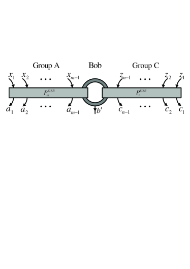
Figure 2: In the nonlocality swapping scheme of two multipartite boxes, Group A and B have $m$-partite and $n$-partite nonlocal correlations respectively. Bob is the common user of two groups. When he applies the coupler on his two boxes and gets a bit 0, the rest users of two groups will share an $m+n-2$-partite GSB.

Bob applies the bipartite coupler $\chi$ on two GSBs and swaps the correlations between two groups of users (FIG.2). Besides Bob, there are $m-1$ and $n-1$ users in group A and C, respectively, which have inputs $x_{1}x_{2}{\cdots}x_{m-1},z_{1}z_{2}{\cdots}z_{n-1}$ and outputs $a_{1}a_{2}{\cdots}a_{m-1},c_{1}c_{2}{\cdots}c_{n-1}$. The coupler acting on two GSBs implements a linear transformation:

$$P_{m}^{\text{GSB}}(a_{1}a_{2}{\cdots}a_{m-1}b_{1}|x_{1}x_{2}{\cdots}x_{m-1}y_{1})P_{n}^{\text{GSB}}(b_{2}c_{1}c_{2}{\cdots}c_{n-1}|y_{2}z_{1}z_{2}{\cdots}z_{n-1})$$ (16)

$$\xrightarrow{\chi}P(a_{1}a_{2}{\cdots}a_{m-1}b^{\prime}c_{1}c_{2}{\cdots}c_{n-1}|x_{1}x_{2}{\cdots}x_{m-1}z_{1}z_{2}{\cdots}z_{n-1})$$

$$=\begin{cases}p(b^{\prime}=0)P_{m+n-2}^{\text{GSB}}(a_{1}a_{2}{\cdots}a_{m-1}c_{1}c_{2}{\cdots}c_{n-1}|x_{1}x_{2}{\cdots}x_{m-1}z_{1}z_{2}{\cdots}z_{n-1}),\\ p(b^{\prime}=1)P^{f}(a_{1}a_{2}{\cdots}a_{m-1}c_{1}c_{2}{\cdots}c_{n-1}|x_{1}x_{2}{\cdots}x_{m-1}z_{1}z_{2}{\cdots}z_{n-1}).\end{cases}$$

The coupler encompasses the inputs and outputs of Bob’s boxes and returns a single bit $b^{\prime}$, Bob succeeds in swapping a generalized Svetlichny correlation between Group A and Group C with probability $p(b^{\prime}=0)=\frac{1}{6}\vec{\text{CHSH}}\cdot\vec{P}(b_{1}b_{2}|y_{1}y_{2})+\frac{1}{3}$, and then an $m+n-2$-partite GSB is generated. If both $m$ and $n$ are greater than $2$, the final correlation is among more users than the initial ones ($m+n-2$ is greater than both $m$ and $n$).

IV.2 Emerge of quantum bound

After swapping the extremal nonlocal boxes, we’ll consider the swapping of noisy correlations. Group A and C now have the multipartite isotropic boxes $P^{\text{GSB}}_{m,\xi}=\xi P^{\text{GSB}}_{m}+(1-\xi)\openone$ and $P^{\text{GSB}}_{n,\xi}=\xi P^{\text{GSB}}_{n}+(1-\xi)\openone$ instead, and Bob will apply the coupler on his two boxes to check whether the quantum bound emerges or not. Fortunately, the answer is positive. the coupling process will be like this:

$$P^{\text{GSB}}_{m,\xi}P^{\text{GSB}}_{n,\xi}\xrightarrow{\chi(b^{\prime}=0)}P^{\text{GSB}}_{m+n-2,\xi^{2}}=\xi^{2}P^{\text{GSB}}_{m+n-2}+(1-\xi^{2})\openone.$$ (17)

By setting the coefficient $\xi=1/\sqrt{2}$, we can get the result that only the postquantum type initial correlations can make the final box nonlocal, which shows the generalized Tsirelson’s bound $\mathcal{B}_{\mathcal{Q}}=2^{(n^{\prime}-1/2)}$ (here $n^{\prime}=m+n-2$) again.

V Swapping many multipartite nonlocality

V.1 Multipartite nonlocality swapping

After presenting the generalization in section IV, we now introduce a more general nonlocality swapping scheme. Bob shares nonlocal boxes with three or more groups of users, and his new purpose is swapping nonlocal correlation between all of the groups. Toward this new goal, Bob makes a feasible try by using bipartite coupler $\chi$. He will show the probability to swap nonlocal correlation between groups of users by demonstrating the simplest example where he shares PR boxes with other three users Alice(A), Charlie(C) and Danny(D).

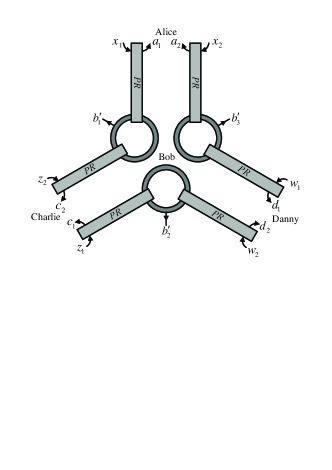
Figure 3: A hybrid scheme for swapping the bipartite PR correlations to tripartite Svetlichny correlation. Bob applies three couplers on six PR boxes, and gets three output bits $b^{\prime}_{1}$, $b^{\prime}_{2}$ and $b^{\prime}_{3}$. Alice, Charlie and Danny applies the local operation: inputs $x_{1}=x_{2}=x$, $z_{1}=z_{2}=z$, $w_{1}=w_{2}=w$ and outputs $a=a_{1}{\oplus}a_{2}$, $c=c_{1}{\oplus}c_{2}$, $d=d_{1}{\oplus}d_{2}$. If $b^{\prime}_{1}=b^{\prime}_{2}=b^{\prime}_{3}=0$, a Svetlichny box is generated from the initial PR boxes.

As depicted in FIG.3, Bob has two copies of PR box with A, C and D each. First, Bob applies the coupler on the boxes he shares with A and C, C and D, A and D separately, and then he will get three outputs after his actions. The process succeeds if the three outputs are all bit $0$. Second, some corresponding local operations (LO) must be applied on A, C and D’s boxes. After that, an Svetlichny correlation is generated between A, C and D.

Suppose that Bob’s correlation $P(b_{1}b_{2}b_{3}|y_{1}y_{2}y_{3})$ is fully mixed correlation, and the transformation of this scheme should be written as:

$$\left.\begin{aligned} P^{\text{PR}}(a_{1}b_{1}|x_{1}y_{1})P^{\text{PR}}(c_{2}b_{2}|z_{2}y_{2})\xrightarrow{\chi,LO}\\ P^{\text{PR}}(c_{1}b_{3}|z_{1}y_{3})P^{\text{PR}}(d_{2}b_{4}|w_{2}y_{4})\xrightarrow{\chi,LO}\\ P^{\text{PR}}(d_{1}b_{5}|w_{1}y_{5})P^{\text{PR}}(a_{2}b_{6}|x_{2}y_{6})\xrightarrow{\chi,LO}\\ \end{aligned}\right\}P(ab^{\prime}_{1}b^{\prime}_{2}b^{\prime}_{3}cd|xzw)$$ (18)

$$=\begin{cases}\frac{1}{27}P^{\text{SB}},&\text{if }b^{\prime}_{1}=b^{\prime}_{2}=b^{\prime}_{3}=0,\\ \frac{6}{27}(\frac{3}{2}\openone-\frac{1}{2}P^{\text{SB}}),&\text{if two of }b^{\prime}_{1},b^{\prime}_{2},b^{\prime}_{3}\text{ equal }0,\\ \frac{12}{27}(\frac{3}{4}\openone+\frac{1}{4}P^{\text{SB}}),&\text{if two of }b^{\prime}_{1},b^{\prime}_{2},b^{\prime}_{3}\text{ equal }1,\\ \frac{8}{27}(\frac{9}{8}\openone-\frac{1}{8}P^{\text{SB}}),&\text{if }b^{\prime}_{1}=b^{\prime}_{2}=b^{\prime}_{3}=1.\\ \end{cases}$$

Analysis of the scheme: In this scheme, Bob realizes a nonlocality swapping scheme, which generates a tripartite nonlocal extremal correlation from initial six bipartite extremal ones. Because three bipartite couplers are applied, the probability of successful swapping is only $1/27$, and it seems too small. This method can be extended to generate multipartite nonlocal correlation from sufficient bipartite ones. $N(N-1)/2$ couplers will act on $N(N-1)$ PR boxes and generate a $N$-partite GSB with probility $1/3^{(N(N-1)/2)}$. In essence, it is a hybrid scheme of Skrzypczyk’s scheme and simulating tripartite boxesresource , and obviously, an less efficient and high consumption scheme. So, we will give another more efficient and low-consumption swapping scheme for many multipartite boxes.

V.2 Swapping many boxes by multipartite coupler $\chi_{N}$

We will present our generalization, a more efficient scheme for multipartite nonlocality swapping than the hybrid one. In this scheme, only one generalized multipartite coupler is needed, and the probability of success is the same as Skrzypczyk’s scheme.

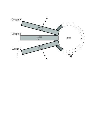
Figure 4: Multipartite coupler for many boxes. Bob applies the coupler on $N$ GSBs and gets a bit $b^{\prime}$. The generalized coupler is an analogue of quantum joint measurement on N particles, among which each comes from a multipartite entangled state in multiparticle entanglement swapping.

Generalized multipartite coupler $\chi_{N}$: In the protocol of multipartite entanglement swappingmultiES , a joint measurement is performed on N particles, among which each comes from a multipartite entangled state, and then a final multipartite entangled state is generated between the rest users. Our generalized coupler applying on many boxes is the analogue of this joint measurement on N particles(see in FIG.4). The coupler $\chi_{N}$ will return a single bit $b^{\prime}$ when applied on $N$ nonlocal boxes, which will be the indication of whether the coupling is success. The probability of output bit $b^{\prime}=0$ is a linear function about the correlations of boxes that the coupler is acting on.

The generalization of nonlocality swapping: Now, Bob get a new device-the multipartite coupler $\chi_{N}$, and he will try to swap nonlocal correlation between many multipartite correlated boxes again.

There are $N$ groups of users and the $i$th ($i=1,2,\cdots,N$) group shares a $n(i)$-partite GSB. Bob is a special user who belongs to every group, and he will carry out the generalized coupler on all boxes. The transformation is defined as follows:

$$P_{n(1)}^{\text{GSB}}(A_{1}b_{1}|X_{1}y_{1})P_{n(2)}^{\text{GSB}}(A_{2}b_{2}|X_{2}y_{2}){\cdots}P_{n(N)}^{\text{GSB}}(A_{N}b_{N}|X_{N}y_{N})$$ (19)

$$\xrightarrow{\chi_{N}}\begin{cases}p(b^{\prime}=0)P_{{\sum}n(i)-N}^{\text{GSB}}(A|X),\\ p(b^{\prime}=1)P^{f}(A|X).\\ \end{cases}$$

Where $A_{i}$ means the $i$th box’s all outputs $a_{1}a_{2}{\cdots}a_{n(i)-1}$ except Bob’s $b_{i}$, and $X_{i}$ means the $i$th box’s inputs $x_{1}x_{2}{\cdots}x_{n(i)-1}$ except Bob’s $y_{i}$. The $A$ and $X$ without subscript mean all users’ input bits and output bits except Bob’s. One $\sum_{i=1}^{N}n(i)-N$-partite correlation will be generated after a successful coupling in Bob’s location.

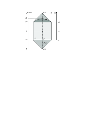
Figure 5: The set of resources for the generalized nonlocality swapping. The left axis is the violation under GSI expression. Local states satisfy $-2^{n-1}\leq\vec{\text{GSI}}\cdot\vec{P}^{L}\leq 2^{n-1}$, the other states have nonlocal correlation otherwise. Generalized Tsirelson’s bound $\mathcal{B}_{\mathcal{Q}}=2^{n-1/2}$ lies on the multipartite isotropic boxes (the dashed line). The right axis is the success probability of the generalized coupler. The coupler is only allowed to be applied on the area: $-2^{n-1}\leq\vec{\text{GSI}}\cdot\vec{P}\leq 2^{n}$. Note the polytope of multipartite resource is a high-dimensional system, while the figure is a two-dimensional illustration.

Suppose that a perfect coupler works on the region of nonsignaling polytope depicted in FIG.5, and then the rest users will get a local correlation which violates the GSI by $-2^{n-1}$ when swapping fails; a GSB will be generated when the coupler returns a single bit $0$. The output is deterministic $1$ when applying the coupler on the failure correlation $P^{f}(A|X)$ and $0$ on generalized Svetlichny correlation. Then the generalized coupler acting on any allowed box gives a successful probability:

$$p(b^{\prime}=0)=\frac{1}{3\cdot 2^{n-1}}\vec{\text{GSI}}\cdot\vec{P}+\frac{1}{3}.$$ (20)

For a natural correlation $\openone$, the optimal probability of success is also $1/3$ as before.

Comments on the generalization: Nonlocality swapping makes it possible to generate multipartite nonlocal correlation from many nonlocal correlations. For instance, we could generate a $4$-partite Svetlichny box from one tripartite Svetlichny box and two PR boxes by a generalized coupler $\chi_{3}$.

The generalized swapping process is also a linear transformation. Let $N=2$, the scheme becomes the one we presented in Sec. IV. And further, let $n(1)=n(2)=2$, it is the same as Skrzypczyk’s scheme.

When the noisy condition is considered, Tsirelson’s bound for quantum nonlocality doesn’t always appear in the swapping process. Basing on the linearity of the swapping, if all group’s correlations are noisy like $P_{\xi}^{\text{GSB}}={\xi}P_{n(i)}^{\text{GSB}}+(1-\xi)\openone$, the final correlation will be $P_{\xi^{N}}^{\text{GSB}}={\xi^{N}}P_{{\sum}n(i)-N}^{\text{GSB}}+(1-\xi^{N})\openone$. The quantum bound only appears in the case where two boxes are noisy or the coupler is $\chi_{2}$.

VI Conclusions

We found that CHSH inequality is also pragmatic for previous nonlocality swapping scheme. Then we focused on the Svetlichny inequality in tripartite system, and showed the form of $N$-Particle Svetlichny inequality in multipartite nonsignaling system. Basing on this generalized Bell-type inequality, we defined the extremal multipartite nonlocal boxes for our generalization of swapping process in the paper.

Using the same coupler applied in Skrzypczyk’s swapping scheme, we first presented a generalized swapping of two arbitrary multipartite nonlocal correlations, which could generate a multipartite correlation with more users than the initial ones. Later, through a combined scheme, we illustrated that multipartite correlation could also be generated from swapping many bipartite boxes. For the sake of efficiency, we finally presented a more general multipartite nonlocality swapping scheme with a generalized multipartite coupler, an analogue of quantum joint measurement in multipartite entanglement swapping. The multipartite coupler builds an efficient device to generate multipartite nonlocal correlation between many users.

The generalized quantum bound always emerges in the scheme of swapping two multipartite isotropic boxes, and occasionally emerges in the process of swapping three or more multipartite boxes. Judged by appearance, the emergence of quantum bound is merely a numerical coincidence, but the mathematical relation between nonlocal criterion ($2^{n-1}$), quantum bound ($2^{n-1/2}$) and extremal violation ($2^{n}$) is a clue to get a deep understanding of quantum nonlocality.

Many open problems are presented in front of us. The fact that nonlocal correlation only can be generated from swapping the postquantum boxes makes not only an emergence of quantum bound but also a gap between QNC and PQC. The coupler, as the most important part in swapping process, beyond the device for poor dynamics applied outside the nosigned boxes after measurement, is very likely valuable for some other dynamical processes, individually or combined as the scheme depicted in FIG.3. How to generalize the swapping to high dimensional systems (multipartite multi-nary boxes) with suitable inequality is worth to study, too.

- (1) A. Einstein, B. Podolsky, and N. Rosen, Phys. Rev. 47, 777 (1935).
- (2) J. S. Bell, Physics (Long Island City, N.Y.) 1, 195 (1964).
- (3) A. Aspect, J. Dalibard, and G. Roger, Phys. Rev. Lett. 49, 1804 (1982).
- (4) W. K. Wootters, Phys. Rev. Lett. 80, 2245 (1998).
- (5) J. S. Clauser, M. A. Horne, A. Shimony, and R. A. Holt, Phys. Rev. Lett. 23, 880 (1969).
- (6) J. F. Clauser and M. A. Horne, Phys. Rev. D 10, 526(1974).
- (7) G. Svetlichny, Phys, Rev. D 35, 3066 (1987).
- (8) S. Popescu and D. Rohrlich, Found. Phys. 24, 379 (1994).
- (9) B. S. Tsirelson, Lett. Math. Phys. 4, 93 (1980).
- (10) J. Barrett, N. Linden, S. Massar, S. Pironio, S. Popescu, and D. Roberts, Phys. Rev. A 71, 022101 (2005).
- (11) L. Masanes, A. Acin, and N. Gisin, Phys. Rev. A 73, 012112 (2006).
- (12) N. Liden, S. Popescu, A. J. Short, and A. Winter, Phys. Rev. Lett. 99, 180502 (2007).
- (13) A. K. Ekert, Phys. Rev. Lett. 67, 661 (1991).
- (14) N. Brunner and P. Skrzypczyk, Phys. Rev. Lett. 102, 160403 (2009).
- (15) H. Buhrman, R. Cleve, S. Massar, and R. de Wolf, Rev. Mod. Phys. 82, 665 (2010).
- (16) M. Forster, S. Winkler, and S. Wolf, Phys. Rev. Lett. 102, 120401. (2009).
- (17) P. Skrzypczyk, N. Brunner, and S. Popescu, Phys. Rev. Lett. 102, 110402 (2009).
- (18) A. J. Short, S. Popescu, and N. Gisin, Phys. Rev. A 73, 012101 (2006).
- (19) P. Skrzypczyk, and N. Brunner, New. J. Phys. 11, 073014 (2009).
- (20) M. Zukowski, A. Zeilinger, M. A. Horne, and A. K. Ekert, Phys. Rev. Lett. 71, 4287 (1993).
- (21) M. Zukowski, A. Zeilinger, and H. Weinfurter, Ann. N. Y. Acad. Sci. 755, 91 (1995).
- (22) S. Bose, V. Vedral, and P. L. Knight, Phys. Rev. A 57, 822 (1998).
- (23) M. Seevinck and G. Svetlichny, Phys. Rev. Lett. 89, 060401 (2002).