On the Condition Number of the Total Least Squares Problem

Abstract

This paper concerns singular value decomposition (SVD)-based computable formulas and bounds for the condition number of the Total Least Squares (TLS) problem. For the TLS problem with the coefficient matrix $A$ and the right-hand side $b$, a new closed formula is presented for the condition number. Unlike an important result in the literature that uses the SVDs of both $A$ and $[A,\ b]$, our formula only requires the SVD of $[A,\ b]$. Based on the closed formula, both lower and upper bounds for the condition number are derived. It is proved that they are always sharp and estimate the condition number accurately. A few lower and upper bounds are further established that involve at most the smallest two singular values of $A$ and of $[A,\ b]$. Tightness of these bounds is discussed, and numerical experiments are presented to confirm our theory and to demonstrate the improvement of our upper bounds over the two upper bounds due to Golub and Van Loan as well as Baboulin and Gratton. Such lower and upper bounds are particularly useful for large scale TLS problems since they require the computation of only a few singular values of $A$ and $[A,\ b]$ other than all the singular values of them.

Keywords: total least squares, perturbation, condition number, singular value decomposition.

AMS subject classification (2000): 65F35, 15A12, 15A18.

1 Introduction

For given $A\in\mathbb{R}^{m\times n}(m>n)$, $b\in\mathbb{R}^{m}$, the total least squares (TLS) problem can be formulated as (see, e.g., [2, 6, 17])

$$\min\|[E,\,f]\|_{F},\text{\quad subject to \quad}b+f\in\mathcal{R}(A+E),$$ (1)

where $\|\cdot\|_{F}$ denotes the Frobenius norm of a matrix and $\mathcal{R}(\cdot)$ denotes the range space. Suppose that $[E_{TLS},\,f_{TLS}]$ solves the above problem. Then $x=x_{TLS}$ that satisfies the equation $(A+E_{TLS})x=b+f_{TLS}$ is called the TLS solution of (1). The TLS problem is a formulation of the linear approximation problem $Ax\approx b$. In this paper, we concentrate on the inconsistent linear approximation problem, i.e., $b\notin{\mathcal{R}(A)}$. Otherwise, $[E_{TLS},\,f_{TLS}]=O$, the zero matrix.

Given a problem, the condition number measures the worst-case sensitivity of its solution to small perturbations in the input data. It is well known that the condition number is independent of perturbations themselves and is expressed by some information about the original data. Combined with backward errors, it provides a (possibly approximate) linear upper bound for the forward error, i.e., the difference between a perturbed solution and the exact solution. Since the 1980’s, algebraic perturbation analysis for the TLS problem has received considerable attention; see [4, 6, 15, 21] and the references therein. From the expressions of perturbation bounds presented in [4, 6, 15, 21], we can see that there are some essential distinctions between them and a standard form. The perturbation bound in [6] is a standard one in the sense that it is expressed as some perturbation independent factor times backward errors. So, this factor is naturally an upper bound for the TLS condition number. The perturbation bound in [21] is nonstandard and unusual since the perturbation bound is not zero when a perturbation is exactly zero. Actually, a careful observation reveals that the bound is never less than a certain positive constant under the assumption $b\notin{\mathcal{R}(A)}$. As a result, it makes no sense to extract an upper bound for the TLS condition number from this perturbation bound. The perturbation bounds in [4, 15] are very different from a standard perturbation bound in that they contain some information about the perturbed TLS problem, e.g., the TLS solution $\tilde{x}_{TLS}$ of the perturbed TLS problem in [4] and the right singular vectors associated with the smallest singular values of both $[A,\ b]$ and its perturbed matrix in [15]. Because of these features and the fact that the condition number itself has nothing to do with perturbations, it is impossible to extract upper bounds for the TLS condition number from the perturbation bounds in [4, 15]. If one attempts to find suitable upper bounds for the TLS condition number, some further and complicated treatments are required and it is necessary to make each of their perturbation bounds become a standard one, that is, some perturbation independent factor times the backward error.

In recent years, asymptotic perturbation analysis and TLS condition numbers have been investigated. Zhou et al. [22] and the authors [14] have presented a first order perturbation analysis of the TLS problem and established Kronecker product-based condition number formulas. Baboulin and Gratton [1] have derived an SVD-based closed formula for the TLS condition number, which involves all the singular values and the right singular vectors of both $A$ and $[A,\,b]$, and an upper bound, which involves only several singular values of $A$ and $[A,\,b]$. To our best knowledge, however, there has been no lower bound available for the TLS condition number in the literature.

It is well known that the TLS solution $x_{TLS}$ involves the smallest singular value and the corresponding right singular vector of $[A,\,b]$, see, e.g., [6]. Very recently, a new classification has been proposed in [9] for the TLS problem in $AX\approx B$ with $B\in\mathbb{R}^{m\times d}$ and $d\geq 1$. It is based on properties of the SVD of the extended matrix $[B,\ A]$ and has established further results on existence and uniqueness of the TLS solution. In this paper, based on the intimate relation between SVDs and TLS problems and motivated by the work of [1], we continue our work in [14] to study SVD-based TLS condition number theory. We will derive a number of results. Firstly, we establish a new closed formula of the TLS condition number. It is distinctive that, unlike the result in [1] that requires the SVDs of both $A$ and $[A,\ b]$, our formula only uses the singular values and the right singular vectors of $[A,\,b]$. Secondly, starting with the closed formula, we present both lower and upper bounds for the condition number that involve the singular values of $[A,\,b]$ and the last entries of the right singular vectors of $[A,\,b]$. Furthermore, we prove that these bounds are always sharp and can estimate the condition number accurately. We then focus on cheaply computable bounds for the TLS condition number. We establish lower and upper bounds that involve at most the smallest two singular values of $A$ and $[A,\ b]$. We discuss how tight the bounds are. These bounds are particularly useful for large scale TLS problems since they require to compute only very few of the smallest singular values of $A$ and $[A,\ b]$ rather than all the singular values of them. So we can compute these bounds by using some iterative solvers for large SVDs, e.g., [11, 12]. From [6], as mentioned previously, an upper bound for the TLS condition number can be extracted. It has been simplified and applied to evaluate the conditioning of the TLS problem in [3]. We will present numerical experiments to demonstrate improvements of our upper bounds over the two upper bounds due to Golub and Van Loan [6] and Baboulin and Gratton [1], respectively.

We mention that for given $A$ and $b$ the standard least squares (LS) problem is always and can be much better conditioned than the corresponding TLS problem; see, e.g., [2, p.180]. The results in this paper allow us to compare the sensitivity of solution of the standard LS problem to the sensitivity of the solution of the TLS problem. So it may be better to solve the LS problem if possible. This is the case when all the errors are confined to the “observation” $b$ but $A$ is assumed to be free of errors. However, this assumption may be unrealistic: sampling errors, human errors, modeling errors and instrument errors often imply inaccuracies of $A$ as well. If both $A$ and $b$ are subject to errors, a reasonable way to take the errors in $A$ into account may be to introduce perturbations also in $A$. The TLS problem (1) is just a natural formulation for this purpose. We refer the reader to [2, 6, 20] for more on the introduction of the TLS problem.

The paper is organized as follows. In Section 2, we present some preliminaries necessary. In Section 3, we establish some useful and necessary results related to a specific orthogonal matrix. In Section 4, we present a new closed formula for the TLS condition number. The bounds for the TLS condition number are derived in Section 5. In Section 6, we report numerical experiments to show the tightness of our bounds for the TLS condition number and improvements over Golub-Van Loan’s bound and Baboulin-Gratton’s bound. We conclude the paper with some remarks and future work in Section 7.

Throughout the paper, for given positive integers $m,n$, denote by $\mathbb{R}^{n}$ the space of $n$-dimensional real column vectors, by $\mathbb{R}^{m\times n}$ the space of all $m\times n$ real matrices, and by $\|\cdot\|$ and $\|\cdot\|_{F}$ the 2-norm and Frobenius norm of their arguments, respectively. Given a matrix $A$, $A(1:i,1:j)$ is a Matlab notation that denotes the submatrix in the intersection of rows $1,\ldots,i$ and columns $1,\ldots,j$, and $\sigma_{i}(A)$ denotes the $i$th largest singular value of $A$. For a vector $a$, $a(i)$ denotes the $i$th component of $a$, and ${\rm{diag}}(a)$ is a diagonal matrix whose diagonals are $a(i)$’s. $I_{n}$ denotes the $n\times n$ identity matrix and $O_{m,n}$ denotes the $m\times n$ zero matrix with $O$ a zero matrix whose dimension is clear from the context. For the matrices $A=[a_{1},\ldots,a_{n}]=[a_{ij}]\in\mathbb{R}^{m\times n}$ and $B$, $A\otimes B=[a_{ij}B]$ is the Kronecker product of $A$ and $B$, and the linear operator ${\rm{vec}}:\mathbb{R}^{m\times n}\rightarrow\mathbb{R}^{mn}$ is defined by ${\rm{vec}}(A)=[a^{T}_{1},\ldots,a^{T}_{n}]^{T}$.

2 Preliminaries

Throughout the paper, let $A=\hat{U}{\rm{diag}}(\hat{\sigma}_{1},\ldots,\hat{\sigma}_{n})\hat{V}^{T}$ be the thin SVD of $A\in\mathbb{R}^{m\times n}$, where $\hat{\sigma}_{1}\geq\cdots\geq\hat{\sigma}_{n}$, $\hat{U}\in\mathbb{R}^{m\times n}$, $\hat{V}\in\mathbb{R}^{n\times n}$ and $\hat{U}^{T}\hat{U}=I_{n}$, $\hat{V}^{T}\hat{V}=I_{n}$, and let $[A,\,b]=U{\rm{diag}}(\sigma_{1},\ldots,\sigma_{n+1})V^{T}$ be the thin SVD of $[A,\,b]\in\mathbb{R}^{m\times(n+1)}$, where $\sigma_{1}\geq\cdots\geq\sigma_{n+1}$, $U=[u_{1},\ldots,u_{n+1}]\in\mathbb{R}^{m\times(n+1)}$, $V=[v_{1},\ldots,v_{n+1}]\in\mathbb{R}^{(n+1)\times(n+1)}$ and $U^{T}U=I_{n+1}$, $V^{T}V=I_{n+1}$.

The TLS problem (1) may not have a solution, but it does have a unique solution if the following condition holds [17]:

$$A\,\,\text{has rank}\,\,n\,\,\text{and}\,\,b\not\perp\mathcal{U}_{min},$$ (2)

where $\mathcal{U}_{min}$ denotes the left singular vector subspace of $A$ corresponding to its smallest singular value. Throughout the paper, we always assume that (2) holds.

It is noted in [17] that condition (2) means $\sigma_{n+1}<\hat{\sigma}_{n}$, the existence and uniqueness condition of the TLS solution given in [6]. Under the condition that $\sigma_{n+1}<\hat{\sigma}_{n}$, it is proved in [6] that

$$x_{TLS} = (A^{T}A-\sigma^{2}_{n+1}I)^{-1}A^{T}b$$ (3)

$$= -\left[\frac{v_{n+1}(1)}{v_{n+1}(n+1)},\ldots,\frac{v_{n+1}(n)}{v_{n+1}(n+1)}\right]^{T}.$$ (4)

We comment that (2) implies that $A^{T}b\neq 0$. So $x_{TLS}\neq 0$.

Given the TLS problem (1), let $\tilde{A}=A+\Delta A$, $\tilde{b}=b+\Delta b$, where $\Delta A$ and $\Delta b$ denote the perturbations in $A$ and $b$, respectively. Consider the perturbed TLS problem

$$\min\|[E,\,f]\|_{F}\,\,\,{\text{subject to}}\,\,\tilde{b}+f\in\mathcal{R}(\tilde{A}+E).$$ (5)

Under the assumption that $b\notin\mathcal{R}(A)$, it follows from (2) that $0<\sigma_{n+1}<\hat{\sigma}_{n}$. In [14], the following result is established for the TLS solution $\tilde{x}_{TLS}$ of the perturbed TLS problem (5).

Theorem 1

Suppose that the TLS problem (1) satisfies $0<\sigma_{n+1}<\hat{\sigma}_{n}$. Define $r=Ax_{TLS}-b$ and $G=[x^{T}_{TLS},\,\,-1]\otimes I_{m}\in\mathbb{R}^{m\times(mn+m)}$. If $\|[\Delta A,\,\,\Delta b]\|_{F}$ is small enough, then the perturbed problem (5) has a unique TLS solution $\tilde{x}_{TLS}$. Moreover,

$$\tilde{x}_{TLS}=x_{TLS}+K~{}\left[\begin{array}[]{c}{\rm{vec}}(\Delta A)\\ \Delta b\\ \end{array}\right]+\mathcal{O}(\|[\Delta A,\,\,\Delta b]\|^{2}_{F}),$$ (6)

where

$$K=\left(A^{T}A-\sigma^{2}_{n+1}I_{n}\right)^{-1}\left(2A^{T}\frac{r}{\|r\|}\frac{r^{T}}{\|r\|}G-A^{T}G-[I_{n}\otimes r^{T},\,O_{n,m}]\right)\in\mathbb{R}^{n\times(mn+m)}.$$ (7)

It is shown in [6] that

$$\sigma^{2}_{n+1}=\frac{\|r\|^{2}}{1+\|x_{TLS}\|^{2}}$$ (8)

and

$$A^{T}r=\frac{\|r\|^{2}}{1+\|x_{TLS}\|^{2}}x_{TLS}=\sigma^{2}_{n+1}x_{TLS}.$$ (9)

From (4), it follows that

$$v_{n+1}=\frac{1}{\sqrt{1+\|x_{TLS}\|^{2}}}\left[\begin{array}[]{c}x_{TLS}\\ -1\\ \end{array}\right]$$ (10)

up to a sign $\pm 1$. We will use the above two relations later. The following basic properties of the Kronecker products of matrices can be found in [8] and are needed later:

$$(A_{1}\otimes A_{3})(A_{2}\otimes A_{4})=(A_{1}A_{2})\otimes(A_{3}A_{4}),$$

$$(A_{1}\otimes A_{2})^{T}=A^{T}_{1}\otimes A^{T}_{2},$$

where $A_{i},i=1,\ldots,4$ are matrices of appropriate sizes.

3 Some results related to a specific orthogonal matrix

In this section, we establish a number of results that are related to a specific orthogonal matrix. They play a central role in deriving our lower and upper bounds for the condition number of the TLS problem in Section 5.

Proposition 1

Let $W$ be an arbitrary $(n+1)\times(n+1)$ orthogonal matrix with $W(n+1,n+1)=-\alpha$, $0<\alpha<1$. Denote $W_{11}=W(1:n,1:n)$. Then

$$\sigma_{1}(W_{11})=\cdots=\sigma_{n-1}(W_{11})=1,\,\,\sigma_{n}({W_{11}})=\alpha.$$ (11)

Furthermore, $W$ can be written as

$$W=\left[\begin{array}[]{cc}W_{11}&\sqrt{1-\alpha^{2}}~{}\bar{u}_{n}\\ \sqrt{1-\alpha^{2}}~{}\bar{v}^{T}_{n}&-\alpha\\ \end{array}\right],$$ (12)

where $\bar{u}_{n}$ and $\bar{v}_{n}$ are the left and right singular vectors associated with the smallest singular value of $W_{11}$.

Proof. It is an immediate result of Theorem 2.6.3 in [7]. $\Box$

Let $[\bar{\beta}_{1},\ldots,\bar{\beta}_{n},-\alpha]$ be the last row of $W$. From (12) we have

$$\bar{v}^{T}_{n}=\frac{1}{\sqrt{1-\alpha^{2}}}[\bar{\beta}_{1},\ldots,\bar{\beta}_{n}].$$ (13)

Since ($\alpha^{-1}$, $\bar{u}_{n}$, $\bar{v}_{n}$) is the largest singular triplet of $W^{-T}_{11}$, from (11) we get the SVD of $W^{-T}_{11}$:

$$W^{-T}_{11}=\alpha^{-1}\bar{u}_{n}\bar{v}^{T}_{n}+\sum^{n-1}_{i=1}\bar{u}_{i}\bar{v}^{T}_{i},$$

where $\bar{u}_{i},\bar{v}_{i},i=1,\ldots,n-1$ represent the left and right singular vectors associated with the singular value one. Then, by (13) we obtain

$$W^{-T}_{11} = \left[\alpha^{-1}\bar{u}_{n},\bar{u}_{1},\ldots,\bar{u}_{n-1}\right]\left[\begin{array}[]{ccc}\frac{\bar{\beta}_{1}}{\sqrt{1-\alpha^{2}}}&\cdots&\frac{\bar{\beta}_{n}}{\sqrt{1-\alpha^{2}}}\\ \bar{v}_{1}(1)&\ldots&\bar{v}_{1}(n)\\ \vdots&\cdots&\vdots\\ \bar{v}_{n-1}(1)&\cdots&\bar{v}_{n-1}(n)\\ \end{array}\right]$$ (18)

$$= \left[\frac{\alpha^{-1}\bar{\beta}_{1}}{\sqrt{1-\alpha^{2}}}\bar{u}_{n}+w_{1},\ldots,\frac{\alpha^{-1}\bar{\beta}_{n}}{\sqrt{1-\alpha^{2}}}\bar{u}_{n}+w_{n}\right],$$ (19)

where $\bar{v}_{i}(k)$ denotes the $k$th component of $\bar{v}_{i}$ and

$$w_{k}=\sum^{n-1}_{i=1}\bar{v}_{i}(k)\bar{u}_{i},\ k=1,\ldots,n.$$ (20)

From (18) we get

$$\sqrt{\sum_{i=1}^{n-1}\bar{v}_{i}^{2}(n)}=\frac{\sqrt{1-\alpha^{2}-\bar{\beta}_{n}^{2}}}{\sqrt{1-\alpha^{2}}},$$ (21)

which will be used later.

Before proceeding, we need the following lemma.

Lemma 1

For given matrices $A_{1},A_{2}\in\mathbb{R}^{n\times n}$, if $A^{T}_{1}A_{2}=O$, then

$$\frac{1}{2}(\|A_{1}\|+\|A_{2}\|)\leq\|A_{1}+A_{2}\|\leq\|A_{1}\|+\|A_{2}\|.$$ (22)

Proof. The upper bound in (22) is obvious. It suffices to prove the lower one. For an arbitrary vector $x\in\mathbb{R}^{n}$, from $(A_{1}x)^{T}(A_{2}x)=0$ it follows that

$$\|A_{1}x\|,\|A_{2}x\|\leq\|A_{1}x+A_{2}x\|$$

and that

$$\|A_{1}\| = {\rm{max}}_{\|x\|=1}\|A_{1}x\|\leq{\rm{max}}_{\|x\|=1}\|A_{1}x+A_{2}x\|=\|A_{1}+A_{2}\|,$$

$$\|A_{2}\| = {\rm{max}}_{\|x\|=1}\|A_{2}x\|\leq{\rm{max}}_{\|x\|=1}\|A_{1}x+A_{2}x\|=\|A_{1}+A_{2}\|.$$

So, the assertion is proved. $\Box$

Now we are in a position to show the following two propositions.

Proposition 2

Let $W$ be an arbitrary $(n+1)\times(n+1)$ orthogonal matrix with $W(n+1,n+1)=-\alpha$, $0<\alpha<1$. Let $W_{11}=W(1:n,1:n)$ and $[\bar{\beta}_{1},\ldots,\bar{\beta}_{n},-\alpha]$ be the last row of $W$. Then for $\bar{S}={\rm{diag}}(\bar{s}_{1},\ldots,\bar{s}_{n})$ with $\bar{s}_{1},\ldots,\bar{s}_{n}$ arbitrary positive numbers ordered as $0<\bar{s}_{1}\leq\bar{s}_{2}\leq\cdots\leq\bar{s}_{n}$, we have

$$\underline{c}:=\frac{1}{2}\left(\frac{\alpha^{-1}\sqrt{\bar{\beta}^{2}_{1}\bar{s}^{2}_{1}+\cdots+\bar{\beta}^{2}_{n}\bar{s}^{2}_{n}}}{\sqrt{1-\alpha^{2}}}+\frac{\sqrt{1-\alpha^{2}-\bar{\beta}^{2}_{n}}}{\sqrt{1-\alpha^{2}}}\bar{s}_{n}\right)$$ (23)

$$\leq \left\|W^{-T}_{11}\bar{S}\right\|\leq\bar{c}:=\frac{\alpha^{-1}\sqrt{\bar{\beta}^{2}_{1}\bar{s}^{2}_{1}+\cdots+\bar{\beta}^{2}_{n}\bar{s}^{2}_{n}}}{\sqrt{1-\alpha^{2}}}+\bar{s}_{n}.$$

Proof. Following (19), we get

$$W^{-T}_{11}\bar{S}=\left[\frac{\alpha^{-1}\bar{\beta}_{1}\bar{s}_{1}}{\sqrt{1-\alpha^{2}}}\bar{u}_{n}+\bar{s}_{1}w_{1},\ldots,\frac{\alpha^{-1}\bar{\beta}_{n}\bar{s}_{n}}{\sqrt{1-\alpha^{2}}}\bar{u}_{n}+\bar{s}_{n}w_{n}\right].$$

Define the matrices

$$A_{1}=\left[\frac{\alpha^{-1}\bar{\beta}_{1}\bar{s}_{1}}{\sqrt{1-\alpha^{2}}}\bar{u}_{n},\ldots,\frac{\alpha^{-1}\bar{\beta}_{n}\bar{s}_{n}}{\sqrt{1-\alpha^{2}}}\bar{u}_{n}\right]$$

and

$$A_{2}=W^{-T}_{11}\bar{S}-A_{1}=\left[\bar{s}_{1}w_{1},\ldots,\bar{s}_{n}w_{n}\right].$$ (24)

Then

$$\|A_{1}\|=\frac{\alpha^{-1}}{\sqrt{1-\alpha^{2}}}\sqrt{\bar{\beta}^{2}_{1}\bar{s}^{2}_{1}+\cdots+\bar{\beta}^{2}_{n}\bar{s}^{2}_{n}}.$$ (25)

From (20) and (21) we obtain

$$\|w_{n}\|=\sqrt{\sum^{n-1}_{i=1}\bar{v}^{2}_{i}(n)}=\frac{\sqrt{1-\alpha^{2}-\bar{\beta}^{2}_{n}}}{\sqrt{1-\alpha^{2}}}\,\mbox{ and }\,\|[w_{1},\ldots,w_{n}]\|=\left\|\sum^{n-1}_{i=1}\bar{u}_{i}\bar{v}^{T}_{i}\right\|=1.$$

Furthermore, since $\|\bar{S}\|=\bar{s}_{n}$, it follows from

$$\|\bar{s}_{n}w_{n}\|\leq\|A_{2}\|\leq\left\|[w_{1},\ldots,w_{n}]\right\|\|\bar{S}\|$$

that

$$\frac{\sqrt{1-\alpha^{2}-{\bar{\beta}}^{2}_{n}}}{\sqrt{1-\alpha^{2}}}\bar{s}_{n}\leq\|A_{2}\|\leq\bar{s}_{n}.$$ (26)

Note that $A^{T}_{1}A_{2}=O$. Based on Lemma 1 and combining (24), (25) with (26), we establish the desired inequality. $\Box$

Proposition 3

Suppose that $0<\alpha\leq\frac{1}{2}$, where $\alpha$ is defined as in Proposition 2. Then for $\underline{c}$ and $\bar{c}$ in Proposition 2, we have

$$\underline{c}<\bar{c}<4\underline{c}.$$ (27)

Proof. If $\frac{|\bar{\beta}_{n}|}{\sqrt{1-\alpha^{2}}}<\frac{\sqrt{3}}{2}$, it is easy to verify that

$$\frac{\sqrt{1-\alpha^{2}-\bar{\beta}^{2}_{n}}}{\sqrt{1-\alpha^{2}}}>\frac{1}{2}$$

and that

$$\underline{c}>\frac{1}{4}\bar{c}.$$

Thus, (27) holds. If $\frac{|\bar{\beta}_{n}|}{\sqrt{1-\alpha^{2}}}\geq\frac{\sqrt{3}}{2}$, then

$$\alpha^{-1}\frac{|\bar{\beta}_{n}|}{\sqrt{1-\alpha^{2}}}\geq\frac{\sqrt{3}}{2}\alpha^{-1}>1,$$

so $\alpha^{-1}\frac{|\bar{\beta}_{n}|}{\sqrt{1-\alpha^{2}}}\bar{s}_{n}>\bar{s}_{n}$, from which and the definitions of $\bar{c}$ and $\underline{c}$ it follows that

$$\bar{c} < \frac{\alpha^{-1}\sqrt{\bar{\beta}^{2}_{1}\bar{s}^{2}_{1}+\cdots+\bar{\beta}^{2}_{n}\bar{s}^{2}_{n}}}{\sqrt{1-\alpha^{2}}}+\alpha^{-1}\frac{|\bar{\beta}_{n}|}{\sqrt{1-\alpha^{2}}}\bar{s}_{n}$$

$$\leq \frac{2\alpha^{-1}\sqrt{\bar{\beta}^{2}_{1}\bar{s}^{2}_{1}+\cdots+\bar{\beta}^{2}_{n}\bar{s}^{2}_{n}}}{\sqrt{1-\alpha^{2}}}$$

$$\leq \frac{2\alpha^{-1}\sqrt{\bar{\beta}^{2}_{1}\bar{s}^{2}_{1}+\cdots+\bar{\beta}^{2}_{n}\bar{s}^{2}_{n}}}{\sqrt{1-\alpha^{2}}}+\frac{2\sqrt{1-\alpha^{2}-\bar{\beta}^{2}_{n}}}{\sqrt{1-\alpha^{2}}}\bar{s}_{n}=4\underline{c}.$$

Thus, (27) holds. $\Box$

This proposition means that the upper bound is at most four times of the lower bound in Proposition 2. So we can estimate $\left\|W^{-T}_{11}\bar{S}\right\|$ accurately by its lower or upper bound within no more than four times of the exact $\left\|W^{-T}_{11}\bar{S}\right\|$.

4 A closed formula for the TLS condition number

Throughout the paper, we follow the definition of condition number in [5, 19]. Let $g:\mathbb{R}^{p}\longrightarrow\mathbb{R}^{q}$ be a continuous map in normed linear spaces defined on an open set $D_{g}\subset\mathbb{R}^{p}$. For a given $a_{0}\in D_{g}$, $a_{0}\neq 0$, with $g(a_{0})\neq 0$, if $g$ is differentiable at $a_{0}$, then the absolute condition number of $g$ at $a_{0}$ is

$$\kappa_{g}(a_{0})=\|g^{\prime}(a_{0})\|,$$ (28)

and the relative condition number is

$$\kappa^{\text{rel}}_{g}(a_{0})=\frac{\|g^{\prime}(a_{0})\|\|a_{0}\|}{\|g(a_{0})\|},$$ (29)

where $g^{\prime}(a_{0})\in\mathbb{R}^{q\times p}$ denotes the Jacobian of $g$ at $a_{0}$.

In [1], an SVD-based closed formula for the condition number of the TLS problem was presented. Denote by $\kappa_{g}(A,b)$ the absolute TLS condition number. It was shown in [1] that

$$\kappa_{g}(A,b)=\sqrt{1+\|x_{TLS}\|^{2}}\left\|\hat{D}~{}[\hat{V}^{T},\,O_{n,1}]~{}V~{}[D,\,O_{n,1}]^{T}\right\|,$$ (30)

where

$$\hat{D} = {\rm{diag}}\left(\frac{1}{\hat{\sigma}^{2}_{1}-\sigma^{2}_{n+1}},\ldots,\frac{1}{\hat{\sigma}^{2}_{n}-\sigma^{2}_{n+1}}\right),$$

$$D = {\rm{diag}}\left(\sqrt{\sigma^{2}_{1}+\sigma^{2}_{n+1}},\ldots,\sqrt{\sigma^{2}_{n}+\sigma^{2}_{n+1}}\right).$$

Next we will derive a new SVD-based formula for the TLS condition number. It is distinctive that, unlike (30) that involves the singular values and right singular vectors of both $[A,\,b]$ and $A$, our formula only uses those of $[A,\,b]$.

Denote $a={\rm{vec}}(A)$ and define the following function in a small neighborhood of $[a^{T},b^{T}]^{T}\in\mathbb{R}^{m(n+1)}$:

$$\begin{array}[]{ccc}g:\mathbb{R}^{m(n+1)}&\longrightarrow&\mathbb{R}^{n}\\ \small{\left[\begin{array}[]{c}\tilde{a}\\ \tilde{b}\\ \end{array}\right]}&\longmapsto&\tilde{x}_{TLS}=(\tilde{A}^{T}\tilde{A}-\tilde{\sigma}^{2}_{n+1}I_{n})^{-1}\tilde{A}^{T}\tilde{b},\end{array}$$

where $\tilde{A}=A+\Delta A$, $\tilde{a}={\rm{vec}}(\tilde{A})=a+{\rm{vec}}(\Delta A)$, $\tilde{b}=b+\Delta b$, and $\tilde{\sigma}_{n+1}=\sigma_{n+1}([\tilde{A},\,\tilde{b}])$. Then we have $g([a^{T},b^{T}]^{T})=x_{TLS}$. Based on Theorem 1, we can present the following result.

Theorem 2

Given the TLS problem (1), let $\kappa_{g}(A,b)$ and $\kappa^{\text{rel}}_{g}(A,b)$ be the absolute and relative condition numbers of the TLS problem, respectively. Then

$$\kappa_{g}(A,b)=\|K\|,\,\,\kappa^{\rm rel}_{g}(A,b)=\frac{\|K\|\|[A,\,b]\|_{F}}{\|x_{TLS}\|},$$ (31)

where $K$ is defined as in (7).

Proof.   Recall that our TLS problem satisfies $0<\sigma_{n+1}<\hat{\sigma}_{n}$. By Theorem 1 and the definition of $g$, we see that $g$ is differentiable at $[a^{T},b^{T}]^{T}$ and $g^{\prime}\left([a^{T},b^{T}]^{T}\right)=K$. Then the assertion follows from (28) and (29) . $\Box$

The formulas for the TLS problem in Theorem 2 depend on Kronecker products of matrices. We comment that the formula for $\kappa^{\rm rel}_{g}(A,b)$ has the same form as that for $\kappa^{K}_{STLS}$ with $\lambda=1$ in Theorem 3.3 of [14], and as stated in [14], mathematically we have $\kappa^{\rm rel}_{g}(A,b)=\kappa^{M}_{STLS}$ when $\lambda=1$ in Theorem 3.1 of [22], where $\kappa^{M}_{STLS}$ is the relative condition number of the Scaled TLS problem with $\lambda$ the scaling factor that is derived in [22].

Now we can establish our computable formula for the TLS condition number.

Theorem 3

Given the TLS problem (1), let $[A,\,b]=U{\rm{diag}}(\sigma_{1},\ldots,\sigma_{n+1})V^{T}$ be the thin SVD of $[A,\,b]$ with $V_{11}=V(1:n,1:n)$. Then

$$\kappa_{g}(A,b)=\sqrt{1+\|x_{TLS}\|^{2}}~{}\|V^{-T}_{11}S\|,$$ (32)

where $S={\rm{diag}}(s_{1},\ldots,s_{n})$ with $s_{i}=\frac{\sqrt{\sigma^{2}_{i}+\sigma^{2}_{n+1}}}{\sigma^{2}_{i}-\sigma^{2}_{n+1}}$, $i=1,\ldots,n$.

Proof. Consider expression (7) of $K$. By the properties of Kronecker product of matrices, we get

$$GG^{T}=\left([x^{T}_{TLS},\,-1]\otimes I_{m}\right)\left(\left[\begin{array}[]{c}x_{TLS}\\ -1\\ \end{array}\right]\otimes I_{m}\right)=(1+\|x_{TLS}\|^{2})I_{m},$$

$$[I_{n}\otimes r^{T},\,O_{n,m}]G^{T}=[I_{n}\otimes r^{T},\,O_{n,m}]\left[\begin{array}[]{c}x_{TLS}\otimes I_{m}\\ -I_{m}\\ \end{array}\right]=(I_{n}\otimes r^{T})(x_{TLS}\otimes I_{m})=x_{TLS}\,r^{T}$$

and

$$[I_{n}\otimes r^{T},\,O_{n,m}]\left[\begin{array}[]{c}I_{n}\otimes r\\ O_{m,n}\\ \end{array}\right]=(I_{n}\otimes r^{T})(I_{n}\otimes r)=\|r\|^{2}I_{n}.$$

Thus, we have

$$\left(2A^{T}\frac{r}{\|r\|}\frac{r^{T}}{\|r\|}G-A^{T}G-[I_{n}\otimes r^{T},\,O_{n,m}]\right)$$

$$\cdot\left(2G^{T}\frac{r}{\|r\|}\frac{r^{T}}{\|r\|}A-G^{T}A-\left[\begin{array}[]{c}I_{n}\otimes r\\ O_{m,n}\\ \end{array}\right]\right)$$

$$= (1+\|x_{TLS}\|^{2})A^{T}A+\|r\|^{2}I_{n}-x_{TLS}r^{T}A-A^{T}rx^{T}_{TLS}$$

$$= (1+\|x_{TLS}\|^{2})A^{T}A+\|r\|^{2}I_{n}-2\sigma^{2}_{n+1}x_{TLS}x^{T}_{TLS},$$

where the last equality uses the relation $A^{T}rx^{T}_{TLS}=\sigma^{2}_{n+1}x_{TLS}x^{T}_{TLS}$, which is obtained from (9). Denote $P=A^{T}A-\sigma^{2}_{n+1}I_{n}$. We get

$$KK^{T} = P^{-1}\left((1+\|x_{TLS}\|^{2})A^{T}A+\|r\|^{2}I_{n}-2\sigma^{2}_{n+1}x_{TLS}x^{T}_{TLS}\right)P^{-1}$$ (36)

$$= (1+\|x_{TLS}\|^{2})P^{-1}\left(A^{T}A+\sigma^{2}_{n+1}I_{n}-\frac{2\sigma^{2}_{n+1}x_{TLS}x^{T}_{TLS}}{1+\|x_{TLS}\|^{2}}\right)P^{-1}$$

$$= (1+\|x_{TLS}\|^{2})\left(P^{-1}+2\sigma^{2}_{n+1}P^{-1}\left(I_{n}-\frac{x_{TLS}x^{T}_{TLS}}{1+\|x_{TLS}\|^{2}}\right)P^{-1}\right),$$ (37)

where the second equality used (8). Denote $V=[v_{1},\ldots,v_{n+1}]$ and note that

$$[A,\,b]^{T}[A,\,b]-\sigma^{2}_{n+1}I_{n+1} = \sum^{n+1}_{i=1}\sigma^{2}_{i}v_{i}v^{T}_{i}-\sigma^{2}_{n+1}\sum^{n+1}_{i=1}v_{i}v^{T}_{i}$$

$$= \sum^{n}_{i=1}(\sigma^{2}_{i}-\sigma^{2}_{n+1})v_{i}v^{T}_{i}.$$

We get

$$P = [I_{n},O]\sum^{n}_{i=1}(\sigma^{2}_{i}-\sigma^{2}_{n+1})v_{i}v^{T}_{i}\left[\begin{array}[]{c}I_{n}\\ O\\ \end{array}\right]$$ (40)

$$= [I_{n},O][v_{1},\ldots,v_{n}]\left[\begin{array}[]{ccc}\sigma^{2}_{1}-\sigma^{2}_{n+1}&&\\ &\ddots&\\ &&\sigma^{2}_{n}-\sigma^{2}_{n+1}\\ \end{array}\right]\left[\begin{array}[]{c}v^{T}_{1}\\ \vdots\\ v^{T}_{n}\\ \end{array}\right]\left[\begin{array}[]{c}I_{n}\\ O\\ \end{array}\right]$$ (49)

$$= V_{11}{\text{diag}}(\sigma^{2}_{1}-\sigma^{2}_{n+1},\ldots,\sigma^{2}_{n}-\sigma^{2}_{n+1})V^{T}_{11}:=V_{11}\Lambda V^{T}_{11}.$$ (50)

Similarly, since $v_{n+1}=\frac{1}{\sqrt{1+\|x_{TLS}\|^{2}}}\left[\begin{array}[]{c}x_{TLS}\\ -1\\ \end{array}\right]$ (c.f. (10)), we have

$$I_{n+1}-\frac{1}{{1+\|x_{TLS}\|^{2}}}\left[\begin{array}[]{cc}x_{TLS}x^{T}_{TLS}&-x_{TLS}\\ -x_{TLS}&1\\ \end{array}\right]=I_{n+1}-v_{n+1}v^{T}_{n+1}=[v_{1},\ldots,v_{n}]\left[\begin{array}[]{c}v^{T}_{1}\\ \vdots\\ v^{T}_{n}\\ \end{array}\right]$$ (56)

and

$$I_{n}-\frac{x_{TLS}x^{T}_{TLS}}{1+\|x_{TLS}\|^{2}}=V_{11}V^{T}_{11}.$$ (57)

Combining (50) and (57), we have

$$P^{-1}+2\sigma^{2}_{n+1}P^{-1}\left(I_{n}-\frac{x_{TLS}x^{T}_{TLS}}{1+\|x_{TLS}\|^{2}}\right)P^{-1}$$

$$= V^{-T}_{11}\Lambda^{-1}V^{-1}_{11}+2\sigma^{2}_{n+1}\left(V^{-T}_{11}\Lambda^{-1}V^{-1}_{11}\right)V_{11}V^{T}_{11}\left(V^{-T}_{11}\Lambda^{-1}V^{-1}_{11}\right)$$

$$= V^{-T}_{11}\Lambda^{-1}V^{-1}_{11}+2\sigma^{2}_{n+1}V^{-T}_{11}\Lambda^{-2}V^{-1}_{11}$$

$$= V^{-T}_{11}\left(\Lambda^{-1}+2\sigma^{2}_{n+1}\Lambda^{-2}\right)V^{-1}_{11}=\left(V^{-T}_{11}S\right)\left(V^{-T}_{11}S\right)^{T}.$$

Then it follows from (37) and Theorem 2 that the desired equality holds. $\Box$

By Theorem 3, we can calculate $\kappa_{g}(A,b)$ by solving a linear system with the coefficient matrix $V^{T}_{11}$. Next we show that the condition number of $V^{T}_{11}$ is exactly $\sqrt{1+\|x_{TLS}\|^{2}}$.

Theorem 4

Under the conditions of Theorem 3, we have

$$\sigma_{1}(V_{11})=\cdots=\sigma_{n-1}(V_{11})=1,\sigma_{n}({V_{11}})=\frac{1}{\sqrt{1+\|x_{TLS}\|^{2}}}$$ (59)

and

$$\kappa(V_{11})=\frac{\sigma_{1}(V_{11})}{\sigma_{n}(V_{11})}=\sqrt{1+\|x_{TLS}\|^{2}}.$$ (60)

Proof. By (10) we get $V(n+1,n+1)=-\frac{1}{\sqrt{1+\|x_{TLS}\|^{2}}}$. Recalling that $x_{TLS}\neq 0$, we get $\frac{1}{\sqrt{1+\|x_{TLS}\|^{2}}}<1$. Applying Proposition 1, we prove the theorem. $\Box$

5 Bounds for the TLS condition number

5.1 Sharp lower and upper bounds based on the SVD of $[A,\,b]$

In this subsection, we apply Theorem 3 and show how to estimate $\kappa_{g}(A,b)$ accurately without computing $\left\|V^{-T}_{11}S\right\|$.

For the TLS problem (1), from now on we denote $\alpha=-V(n+1,n+1)$. By (10) we get

$$\alpha=\frac{1}{\sqrt{1+\|x_{TLS}\|^{2}}}.$$ (61)

Recalling that $x_{TLS}\not=0$, we have $0<\alpha<1$. Then we have the following theorem.

Theorem 5

For the TLS problem (1), it holds that

$$\underline{\kappa}:=\alpha^{-1}\frac{\sqrt{\sigma^{2}_{n}+\sigma^{2}_{n+1}}}{\sigma^{2}_{n}-\sigma^{2}_{n+1}}\leq\kappa_{g}(A,b)\leq\bar{\kappa}:=\alpha^{-2}\frac{\sqrt{\sigma^{2}_{n}+\sigma^{2}_{n+1}}}{\sigma^{2}_{n}-\sigma^{2}_{n+1}}.$$ (62)

Proof. As before, let $[A,\,b]=U{\rm{diag}}(\sigma_{1},\ldots,\sigma_{n+1})V^{T}$ be its thin SVD with $V_{11}=V(1:n,1:n)$. From (59) and (61) it follows that

$$\sigma_{n}(V^{-T}_{11})=\left(\sigma_{1}(V_{11})\right)^{-1}=1,\,\,\sigma_{1}(V^{-T}_{11})=\left(\sigma_{n}(V_{11})\right)^{-1}=\alpha^{-1}.$$ (63)

Define $S={\rm{diag}}(s_{1},\ldots,s_{n})$ with $s_{i}=\frac{\sqrt{\sigma^{2}_{i}+\sigma^{2}_{n+1}}}{\sigma^{2}_{i}-\sigma^{2}_{n+1}}$, $i=1,\ldots,n$. We then have

$$s_{n}=\sigma_{n}(V^{-T}_{11})\|S\|\leq\|V^{-T}_{11}S\|\leq\|V^{-T}_{11}\|\|S\|=\alpha^{-1}s_{n}.$$

Therefore, by Theorem 3 we get the desired inequality. $\Box$

We see that in (62) the ratio of the upper bound and the lower bound is $\frac{1}{\alpha}$. As a consequence, both the bounds estimate $\kappa_{g}(A,b)$ within $\frac{1}{\alpha}$ times. Therefore, if $\alpha\in(0,1)$ is not small, say $\frac{1}{2}<\alpha<1$, both the bounds are very tight and they estimate $\kappa_{g}(A,b)$ accurately.

Starting with (30), Baboulin and Gratton [1, Corollary 1] have derived the following upper bound

$$\kappa_{g}(A,b)\leq\alpha^{-1}\frac{\sqrt{\sigma_{1}^{2}+\sigma_{n+1}^{2}}}{\hat{\sigma}_{n}^{2}-\sigma_{n+1}^{2}}:=\bar{\kappa}(A,b),$$ (64)

which uses $\hat{\sigma}_{n}-\sigma_{n+1}$ to estimate the conditioning of $x_{TLS}$. The smaller $\hat{\sigma}_{n}-\sigma_{n+1}$ is, the possibly worse conditioned the TLS problem is. It has two distinctions with our lower and upper bounds in (62). First, (64) involves the SVDs of both $A$ and $[A,\ b]$ while (62) only makes use of that of $[A,\ b]$. Second, since $\hat{\sigma}^{2}_{n}-\sigma^{2}_{n+1}\leq\sigma^{2}_{n}-\sigma^{2}_{n+1}$ and $\sigma_{1}\geq\sigma_{n}$, our lower and upper bounds can be considerably more accurate than (64) for $\alpha$ not small. We now present a family of examples to illustrate it and the tightness of the bounds in (62) for $\frac{1}{2}<\alpha<1$.

$e_{p}$	$\alpha$	$\hat{\sigma}_{n}-\sigma_{n+1}$	$\kappa_{g}(A,b)$	$~{}\alpha^{-1}\frac{\sqrt{\sigma^{2}_{n}+\sigma^{2}_{n+1}}}{\sigma^{2}_{n}-\sigma^{2}_{n+1}}~{}$	$~{}\alpha^{-2}\frac{\sqrt{\sigma^{2}_{n}+\sigma^{2}_{n+1}}}{\sigma^{2}_{n}-\sigma^{2}_{n+1}}~{}$	$\alpha^{-1}\frac{\sqrt{\sigma_{1}^{2}+\sigma_{n+1}^{2}}}{\hat{\sigma}_{n}^{2}-\sigma_{n+1}^{2}}~{}$
$10^{-3}$	$~{}0.516~{}$	$9.89\times 10^{-4}$	$1.38\times 10^{3}$	$1.37\times 10^{3}$	$2.66\times 10^{3}$	$4.16\times 10^{5}$
$10^{-7}$	$~{}0.792~{}$	$9.99\times 10^{-8}$	$8.93\times 10^{6}$	$8.93\times 10^{6}$	$1.13\times 10^{7}$	$2.54\times 10^{9}$
$10^{-10}$	$~{}0.859~{}$	$1.00\times 10^{-10}$	$8.24\times 10^{9}$	$8.23\times 10^{9}$	$9.59\times 10^{9}$	$2.33\times 10^{12}$

Example. We construct TLS problems as in [1, Example 1]: Define

$$[A,\,b]=Q\left[\begin{array}[]{c}\Sigma\\ O\\ \end{array}\right]V^{T}\in\mathbb{R}^{m\times(n+1)},\,Q=I_{m}-2yy^{T},\,V=I_{n+1}-2zz^{T},$$

where $y\in\mathbb{R}^{m}$ and $z\in\mathbb{R}^{n+1}$ are random unit vectors, and $\Sigma={\text{diag}}(n,n-1,\ldots,1,1-e_{p})$ for a given parameter $e_{p}$. Note that $e_{p}=\sigma_{n}-\sigma_{n+1}$. We have $e_{p}\geq\hat{\sigma}_{n}-\sigma_{n+1}$. By taking small values of $e_{p}$, we get different TLS problems whose conditioning becomes worse and condition number becomes larger as $e_{p}$ becomes smaller. Fixing $m=100$, $n=20$, and taking $e_{p}=10^{-3},10^{-7},10^{-10}$, respectively, we get three different TLS problems whose solutions are computed by the SVD of $[A,\ b]$ and (4). As indicated by the results of $\kappa_{g}(A,b)$, as $e_{p}$ decreases, the TLS problem becomes worse conditioned. This is also reflected by the decay of $\hat{\sigma}_{n}-\sigma_{n+1}$; see (64), and Theorems 8–9 and [6]. Since the $\alpha$’s are bigger than $0.5$ and not small, the lower and upper bounds in (62) estimate the TLS condition numbers accurately, and they are much sharper than bound (64) by roughly two to three orders.

In view of (62) and the comments after its proof as well as the above example, it is only possible and significant to improve the bounds essentially for the case that $\alpha$ is small relative to one. Without loss of generality, we assume that

$$0<\alpha\leq\frac{1}{2}.$$ (65)

It will appear that we can establish some lower bound $\underline{\kappa}$ and upper bound $\bar{\kappa}$ such that $\underline{\kappa}<\bar{\kappa}<4\underline{\kappa}$ holds. As a result, together with (62), we can estimate the TLS condition number $\kappa_{g}(A,b)$ accurately.

Theorem 6

Given the TLS problem (1), let $[A,\,b]=U{\rm{diag}}(\sigma_{1},\ldots,\sigma_{n+1})V^{T}$ be its thin SVD. Denote $[\beta_{1},\ldots,\beta_{n},-\alpha]$ be the last row of $V$ and $S={\rm{diag}}(s_{1},\ldots,s_{n})$, $s_{i}=\frac{\sqrt{\sigma^{2}_{i}+\sigma^{2}_{n+1}}}{\sigma^{2}_{i}-\sigma^{2}_{n+1}}$, $i=1,\ldots,n$. Then

$$\underline{\kappa}:=\frac{1}{2}\left(\frac{\alpha^{-2}\sqrt{\beta^{2}_{1}s^{2}_{1}+\cdots+\beta^{2}_{n}s^{2}_{n}}}{\sqrt{1-\alpha^{2}}}+\frac{\sqrt{1-\alpha^{2}-\beta^{2}_{n}}}{\sqrt{1-\alpha^{2}}}\alpha^{-1}s_{n}\right)$$

$$\leq \kappa_{g}(A,b)\leq\bar{\kappa}:=\frac{\alpha^{-2}\sqrt{\beta^{2}_{1}s^{2}_{1}+\cdots+\beta^{2}_{n}s^{2}_{n}}}{\sqrt{1-\alpha^{2}}}+\alpha^{-1}s_{n}.$$

Moreover, if $0<\alpha\leq\frac{1}{2}$, then

$$\underline{\kappa}<\bar{\kappa}<4\underline{\kappa}.$$

Proof. Recall that $0<\alpha<1$. Noticing that $0<s_{1}\leq s_{2}\leq\cdots\leq s_{n}$ and applying Proposition 2, we have

$$\frac{1}{2}\left(\frac{\alpha^{-1}\sqrt{\beta^{2}_{1}s^{2}_{1}+\cdots+\beta^{2}_{n}s^{2}_{n}}}{\sqrt{1-\alpha^{2}}}+\frac{\sqrt{1-\alpha^{2}-\beta^{2}_{n}}}{\sqrt{1-\alpha^{2}}}s_{n}\right)$$

$$\leq \left\|V^{-T}_{11}S\right\|\leq\frac{\alpha^{-1}\sqrt{\beta^{2}_{1}s^{2}_{1}+\cdots+\beta^{2}_{n}s^{2}_{n}}}{\sqrt{1-\alpha^{2}}}+s_{n},$$

where $V_{11}=V(1:n,1:n)$. By Theorem 3, we get the first part of the theorem. Furthermore, we obtain the second part of the theorem by Proposition 3. $\Box$

The significance of this theorem is that we can estimate the condition number $\kappa_{g}(A,b)$ accurately by its lower or upper bound without calculating $\|V^{-T}_{11}S\|$, i.e., solving the matrix equation $V_{11}^{T}W=S$ for $W$ and computing the 2-norm of $W$, which is expensive when $n$ is large.

5.2 Lower and upper bounds based on a few singular values of $A$ and $[A,\,b]$

In [16], some bounds for the condition number of the Tikhonov regularization solution have been established using only a few singular values of $A$, where $A$ is the coefficient matrix of the least squares problem under consideration. Such kind of bounds are particularly appealing for large scale TLS problems, because the condition number in Theorem 3 and the bounds in Theorem 6 involve all the singular values of $[A,b]$ and are impractical for computational purpose.

Actually, we have presented such kind of bound (62), but as we commented there, for small $\alpha$, the bounds may overestimate or underestimate $\kappa_{g}(A,b)$. In the following, we establish some new lower and upper bounds in the same spirit and finally achieve sharper lower and upper bounds for the case of $0<\alpha\leq\frac{1}{2}$.

Theorem 7

For the TLS problem (1), we have

$$\underline{\kappa}_{1}\leq\kappa_{g}(A,b)\leq\bar{\kappa}_{1},$$ (66)

where

$$\underline{\kappa}_{1}=\alpha^{-1}\frac{\sqrt{\hat{\sigma}^{2}_{n-1}+\sigma^{2}_{n+1}}}{\hat{\sigma}^{2}_{n-1}-\sigma^{2}_{n+1}},\,\,\bar{\kappa}_{1}=\alpha^{-1}\frac{\sqrt{\hat{\sigma}^{2}_{n}+\sigma^{2}_{n+1}}}{\hat{\sigma}^{2}_{n}-\sigma^{2}_{n+1}}.$$ (67)

Proof. Recall that $r=Ax_{TLS}-b$. Denote

$$M=(A^{T}A-\sigma^{2}_{n+1}I_{n})^{-1}\left((1+\|x_{TLS}\|^{2})A^{T}A+\|r\|^{2}I_{n}\right)(A^{T}A-\sigma^{2}_{n+1}I_{n})^{-1}.$$

From (36), we have

$$KK^{T}=M-2\sigma^{2}_{n+1}(A^{T}A-\sigma^{2}_{n+1}I_{n})^{-1}x_{TLS}x^{T}_{TLS}(A^{T}A-\sigma^{2}_{n+1}I_{n})^{-1}.$$ (68)

From now on, denote by $\lambda_{i}(M)$ the $i$th algebraically largest eigenvalue of $M$, where $M$ is an arbitrary symmetric matrix. By the Courant-Fischer theorem [10, p. 182], we get

$$\lambda_{2}(M)\leq\lambda_{1}(KK^{T}).$$ (69)

Furthermore, since $2\sigma^{2}_{n+1}(A^{T}A-\sigma^{2}_{n+1}I_{n})^{-1}x_{TLS}x^{T}_{TLS}(A^{T}A-\sigma^{2}_{n+1}I_{n})^{-1}$ is nonnegative definite, the following inequality holds

$$\lambda_{1}(KK^{T})\leq\lambda_{1}(M).$$ (70)

Combining (69) with (70) and based on (31), we have

$$\sqrt{\lambda_{2}(M)}\leq\kappa_{g}(A,b)\leq\sqrt{\lambda_{1}(M)}.$$

It is easy to verify that the eigenvalues of $M$ form the set

$$\left\{\frac{(1+\|x_{TLS}\|^{2})\hat{\sigma}^{2}_{j}+\|r\|^{2}}{(\hat{\sigma}^{2}_{j}-\sigma^{2}_{n+1})^{2}}\right\}^{n}_{j=1}.$$

We define the function

$$h(\sigma)=\frac{(1+\|x_{TLS}\|^{2}){\sigma}^{2}+\|r\|^{2}}{({\sigma}^{2}-\sigma^{2}_{n+1})^{2}},\,\,\sigma>\sigma_{n+1}$$

and differentiate it to get

$$h^{\prime}(\sigma)=\frac{-2\sigma^{3}(1+\|x_{TLS}\|^{2})-2\sigma(1+\|x_{TLS}\|^{2})\sigma^{2}_{n+1}-4\sigma\|r\|^{2}}{(\sigma^{2}-\sigma^{2}_{n+1})^{3}}.$$

It is seen that $h^{\prime}(\sigma)<0$ and $h(\sigma)$ is decreasing in the interval $(\sigma_{n+1},\infty)$. Thus, we get

$$\lambda_{1}(M)=\frac{(1+\|x_{TLS}\|^{2})\hat{\sigma}^{2}_{n}+\|r\|^{2}}{(\hat{\sigma}^{2}_{n}-\sigma^{2}_{n+1})^{2}},\,\,\lambda_{2}(M)=\frac{(1+\|x_{TLS}\|^{2})\hat{\sigma}^{2}_{n-1}+\|r\|^{2}}{(\hat{\sigma}^{2}_{n-1}-\sigma^{2}_{n+1})^{2}}$$

and

$$\frac{\sqrt{(1+\|x_{TLS}\|^{2})\hat{\sigma}^{2}_{n-1}+\|r\|^{2}}}{\hat{\sigma}^{2}_{n-1}-\sigma^{2}_{n+1}}\leq\kappa_{g}(A,b)\leq\frac{\sqrt{(1+\|x_{TLS}\|^{2})\hat{\sigma}^{2}_{n}+\|r\|^{2}}}{\hat{\sigma}^{2}_{n}-\sigma^{2}_{n+1}}.$$

Recalling (61) and that $\frac{\|r\|^{2}}{1+\|x_{TLS}\|^{2}}=\sigma^{2}_{n+1}$ completes the proof. $\Box$

Remark. Since $\hat{\sigma}_{n}\leq\sigma_{n}$ and $\sigma_{n}\leq\sigma_{1}$, we have proved that

$$\bar{\kappa}_{1}\leq\alpha^{-1}\frac{\sqrt{\sigma_{1}^{2}+\sigma_{n+1}^{2}}}{\hat{\sigma}_{n}^{2}-\sigma_{n+1}^{2}}:=\bar{\kappa}(A,b),$$ (71)

which is just the upper bound (64) derived by Baboulin and Gratton [1]. Therefore, our upper bound $\bar{\kappa}_{1}$ in (67) is always sharper than Baboulin-Gratton’s bound. Moreover, the improvement must be significant when $\frac{\sigma_{1}}{\hat{\sigma}_{n}}>1$ considerably.

It is seen that the lower and upper bounds in Theorem 7 are marginally different provided that $\hat{\sigma}_{n}$ and $\hat{\sigma}_{n-1}$ are close. This means that in this case both bounds are very tight. For the case that $\hat{\sigma}_{n}$ and $\hat{\sigma}_{n-1}$ are not close, we next give a new lower bound that can be better than that in Theorem 7.

Theorem 8

It holds that

$$\underline{\kappa}_{2}\leq\kappa_{g}(A,b)\leq\bar{\kappa}_{1},$$

where $\bar{\kappa}_{1}$ is defined as in Theorem 7 and

$$\underline{\kappa}_{2}=\frac{1}{\alpha\sqrt{{\hat{\sigma}}^{2}_{n}-\sigma^{2}_{n+1}}}.$$

Moreover, when $\hat{\sigma}_{n-1}\geq\sigma_{n+1}+\sqrt{{\hat{\sigma}}^{2}_{n}-\sigma^{2}_{n+1}}$, we have

$$\underline{\kappa}_{1}\leq\underline{\kappa}_{2}.$$

Proof. Denote $P=A^{T}A-\sigma^{2}_{n+1}I_{n}$. From (37), we have

$$\frac{1}{1+\|x_{TLS}\|^{2}}~{}KK^{T}=P^{-1}+2\sigma^{2}_{n+1}P^{-1}\left(I_{n}-\frac{x_{TLS}x^{T}_{TLS}}{1+\|x_{TLS}\|^{2}}\right)P^{-1}.$$

Since the second term in the right-hand side of the above relation is positive definite, we have

$$(1+\|x_{TLS}\|^{2})\lambda_{1}(P^{-1})\leq\lambda_{1}(~{}KK^{T}),$$

that is,

$$\frac{1+\|x_{TLS}\|^{2}}{{\hat{\sigma}^{2}_{n}}-\sigma^{2}_{n+1}}\leq\kappa^{2}_{g}(A,b),$$

which used (31). Thus, recalling (61), we obtain the first part of the theorem.

The second part of the theorem is obtained by noting that

$$\frac{\sqrt{\hat{\sigma}^{2}_{n-1}+\sigma^{2}_{n+1}}}{\hat{\sigma}^{2}_{n-1}-\sigma^{2}_{n+1}}<\frac{1}{\hat{\sigma}_{n-1}-\sigma_{n+1}}\leq\frac{1}{\sqrt{{\hat{\sigma}}^{2}_{n}-\sigma^{2}_{n+1}}}$$

under the assumption that $\hat{\sigma}_{n-1}-\sigma_{n+1}\geq\sqrt{{\hat{\sigma}}^{2}_{n}-\sigma^{2}_{n+1}}$. $\Box$

Remark 1. At a first glance, the assumption in the second part of the theorem seems not so direct but we can justify that it indeed implies that $\hat{\sigma}_{n}$ and $\hat{\sigma}_{n-1}$ are not close. Actually, it is direct to verify that the second part of Theorem 8 holds under the slightly stronger but much simpler condition that

$$\hat{\sigma}_{n-1}\geq 2\hat{\sigma}_{n}.$$

Remark 2. From

$$\frac{\bar{\kappa}_{1}}{\underline{\kappa}_{2}}=\frac{\sqrt{\hat{\sigma}^{2}_{n}+\sigma^{2}_{n+1}}}{\sqrt{\hat{\sigma}^{2}_{n}-\sigma^{2}_{n+1}}}=\sqrt{\frac{1+\frac{\sigma^{2}_{n+1}}{\hat{\sigma}^{2}_{n}}}{1-\frac{\sigma^{2}_{n+1}}{\hat{\sigma}^{2}_{n}}}},$$

it is seen that $\frac{\bar{\kappa}_{1}}{\underline{\kappa}_{2}}>1$ provided that $\sigma_{n+1}>0$. Only for $\sigma_{n+1}=0$, $\bar{\kappa}_{1}=\underline{\kappa}_{2}$ holds. Then, $b\in\mathcal{R}(A)$ and $r=0$.

We observe from the above Remark 2 that the bounds for $\kappa_{g}(A,b)$ in Theorem 8 are tight when $\frac{\sigma_{n+1}}{\hat{\sigma}_{n}}$ is considerably smaller than one. On the other hand, if $\frac{\sigma_{n+1}}{\hat{\sigma}_{n}}$ is not small, these bounds may not be tight. For this case, we will present a new upper bound for better estimating $\kappa_{g}(A,b)$.

Keep (61) and (65) in mind. Based on Propositions 2–3, we establish the following theorem.

Theorem 9

If $0<\alpha\leq\frac{1}{2}$, then

$$\underline{\kappa}_{2}:=\frac{1}{\alpha\sqrt{\hat{\sigma}^{2}_{n}-\sigma^{2}_{n+1}}}\leq\kappa_{g}(A,b)<\bar{\kappa}_{2}:=\sqrt{\frac{1+31\rho^{2}}{1-\rho^{2}}}\frac{1}{\alpha\sqrt{\hat{\sigma}^{2}_{n}-\sigma^{2}_{n+1}}},$$ (72)

where $\rho=\frac{\sigma_{n+1}}{\sigma_{n}}$.

Proof.  The lower bound is the same as that in Theorem 8. We only need to prove the right-hand side of (72). As before, let $[A,\,b]=U{\rm{diag}}(\sigma_{1},\ldots,\sigma_{n+1})V^{T}$ be its thin SVD with $V_{11}=V(1:n,1:n)$. From (37), (50) and (4), we get

$$\frac{1}{1+\|x_{TLS}\|^{2}}~{}KK^{T} = P^{-1}+2\sigma^{2}_{n+1}P^{-1}\left(I_{n}-\frac{x_{TLS}x^{T}_{TLS}}{1+\|x_{TLS}\|^{2}}\right)P^{-1},$$ (73)

$$= V^{-T}_{11}\Lambda^{-1}V^{-1}_{11}+2\sigma^{2}_{n+1}V^{-T}_{11}\Lambda^{-2}V^{-1}_{11}:=P^{-1}+C,$$

where $P=A^{T}A-\sigma^{2}_{n+1}I_{n}$, $\Lambda={\rm{diag}}(\sigma^{2}_{1}-\sigma^{2}_{n+1},\ldots,\sigma^{2}_{n}-\sigma^{2}_{n+1})$. Denote

$$D = {\rm{diag}}(d_{1},\ldots,d_{n}),\,d_{i}=\frac{\sigma_{n+1}}{\sigma^{2}_{i}-\sigma^{2}_{n+1}},i=1,\ldots,n,$$

$$T = {\rm{diag}}(t_{1},\ldots,t_{n}),\,t_{i}=\frac{1}{\sqrt{\sigma^{2}_{i}-\sigma^{2}_{n+1}}},i=1,\ldots,n.$$

Then $P^{-1}=\left(V^{-T}_{11}T\right)\left(TV^{-1}_{11}\right)$ and $C=2\left(V^{-T}_{11}D\right)\left(DV^{-1}_{11}\right)$.

Note that $0<d_{1}\leq d_{2}\leq\cdots\leq d_{n}$ and $0<t_{1}\leq t_{2}\leq\cdots\leq t_{n}$. From Proposition 2, we get

$$\frac{1}{2}\left(\frac{\alpha^{-1}\sqrt{\beta^{2}_{1}d^{2}_{1}+\cdots+\beta^{2}_{n}d^{2}_{n}}}{\sqrt{1-\alpha^{2}}}+\frac{\sqrt{1-\alpha^{2}-\beta^{2}_{n}}}{\sqrt{1-\alpha^{2}}}d_{n}\right)$$ (74)

$$\leq \left\|V^{-T}_{11}D\right\|\leq\frac{\alpha^{-1}\sqrt{\beta^{2}_{1}d^{2}_{1}+\cdots+\beta^{2}_{n}d^{2}_{n}}}{\sqrt{1-\alpha^{2}}}+d_{n}$$

and

$$\frac{1}{2}\left(\frac{\alpha^{-1}\sqrt{\beta^{2}_{1}t^{2}_{1}+\cdots+\beta^{2}_{n}t^{2}_{n}}}{\sqrt{1-\alpha^{2}}}+\frac{\sqrt{1-\alpha^{2}-\beta^{2}_{n}}}{\sqrt{1-\alpha^{2}}}t_{n}\right)$$

$$\leq \left\|V^{-T}_{11}T\right\|\leq\frac{\alpha^{-1}\sqrt{\beta^{2}_{1}t^{2}_{1}+\cdots+\beta^{2}_{n}t^{2}_{n}}}{\sqrt{1-\alpha^{2}}}+t_{n},$$

respectively, where $[\beta_{1},\ldots,\beta_{n},-\alpha]$ is the last row of $V$ as defined previously. Define $k_{n}=\frac{d_{n}}{t_{n}}=\frac{\sigma_{n+1}}{\sqrt{\sigma^{2}_{n}-\sigma^{2}_{n+1}}}$. Then

$$\frac{d_{1}}{t_{1}}=\frac{\sigma_{n+1}}{\sqrt{\sigma^{2}_{1}-\sigma^{2}_{n+1}}}\leq k_{n}\,,\ldots,\frac{d_{n-1}}{t_{n-1}}=\frac{\sigma_{n+1}}{\sqrt{\sigma^{2}_{n-1}-\sigma^{2}_{n+1}}}\leq k_{n}.$$

Thus, from (74) we get

$$\frac{1}{\sqrt{2}}\|C\|^{\frac{1}{2}}=\left\|V^{-T}_{11}D\right\|\leq k_{n}\left(\frac{\alpha^{-1}\sqrt{\beta^{2}_{1}t^{2}_{1}+\cdots+\beta^{2}_{n}t^{2}_{n}}}{\sqrt{1-\alpha^{2}}}+t_{n}\right).$$ (75)

For the lower and upper bounds on $\left\|V^{-T}_{11}T\right\|$ above, Propositions 2–3 tell us that

$$\frac{\alpha^{-1}\sqrt{\beta^{2}_{1}t^{2}_{1}+\cdots+\beta^{2}_{n}t^{2}_{n}}}{\sqrt{1-\alpha^{2}}}+t_{n} < 2\left(\frac{\alpha^{-1}\sqrt{\beta^{2}_{1}t^{2}_{1}+\cdots+\beta^{2}_{n}t^{2}_{n}}}{\sqrt{1-\alpha^{2}}}+\frac{\sqrt{1-\alpha^{2}-\beta^{2}_{n}}}{\sqrt{1-\alpha^{2}}}t_{n}\right)$$ (76)

$$< 4\left\|V^{-T}_{11}T\right\|.$$

Therefore, based on (75) and (76), we obtain

$$\frac{1}{\sqrt{2}}\|C\|^{\frac{1}{2}}<4k_{n}\left\|V^{-T}_{11}T\right\|=4k_{n}\|P^{-1}\|^{\frac{1}{2}}$$

and

$$\|C\|<32k^{2}_{n}\|P^{-1}\|.$$ (77)

Combining (73) with (77) and based on (31), we get

$$\kappa_{g}(A,b)=\|K\|=\|KK^{T}\|^{\frac{1}{2}} < \sqrt{1+32k^{2}_{n}}\sqrt{1+\|x_{TLS}\|^{2}}\|P^{-1}\|^{\frac{1}{2}}$$

$$= \sqrt{\frac{1+31\rho^{2}}{1-\rho^{2}}}\frac{\sqrt{1+\|x_{TLS}\|^{2}}}{\sqrt{\hat{\sigma}^{2}_{n}-\sigma^{2}_{n+1}}}$$

$$= \sqrt{\frac{1+31\rho^{2}}{1-\rho^{2}}}\frac{1}{\alpha\sqrt{\hat{\sigma}^{2}_{n}-\sigma^{2}_{n+1}}},$$

where the last equality uses (61). $\Box$

Remark. It is clear that the bounds in Theorem 9 are tight when $\rho=\frac{\sigma_{n+1}}{\sigma_{n}}$ is considerably smaller than one. Note that the lower and upper bounds in Theorem 8 differ considerably when $\frac{\sigma_{n+1}}{\hat{\sigma}_{n}}$ is close to one. The result in this theorem is of particular importance when $\frac{\sigma_{n+1}}{\hat{\sigma}_{n}}$ is close to one, since the upper bound here can be considerably sharper than the upper bound of Theorem 8 when $\rho=\frac{\sigma_{n+1}}{\sigma_{n}}$ is small.

The improvement of $\bar{\kappa}_{2}$ over $\bar{\kappa}_{1}$ can be illustrated as follows. For $\rho=\frac{\sigma_{n+1}}{\sigma_{n}}$ small, we have

$$\bar{\kappa}^{\text{rel}}_{2}:=\frac{\bar{\kappa}_{2}}{\|x_{TLS}\|}\|[A,\,b]\|_{F} = \sqrt{\frac{1+31\rho^{2}}{1-\rho^{2}}}\frac{\sqrt{1+\|x_{TLS}\|^{2}}}{\|x_{TLS}\|}\frac{\|[A,\,b]\|_{F}}{\sqrt{\hat{\sigma}^{2}_{n}-\sigma^{2}_{n+1}}},$$

an upper bound for $\kappa^{\text{rel}}_{g}(A,b)$, is a moderate multiple of $\frac{1}{\sqrt{\hat{\sigma}^{2}_{n}-\sigma^{2}_{n+1}}}$, while

$$\bar{\kappa}^{\text{rel}}_{1}:=\frac{\bar{\kappa}_{1}}{\|x_{TLS}\|}\|[A,\,b]\|_{F} = \frac{\sqrt{1+\|x_{TLS}\|^{2}}}{\|x_{TLS}\|}\frac{\sqrt{\hat{\sigma}^{2}_{n}+\sigma^{2}_{n+1}}}{\hat{\sigma}^{2}_{n}-\sigma^{2}_{n+1}}\|[A,\,b]\|_{F}$$

is a moderate multiple of $\frac{1}{\hat{\sigma}^{2}_{n}-\sigma^{2}_{n+1}}$. So the improvement of $\bar{\kappa}^{\text{rel}}_{2}$ over $\bar{\kappa}^{\text{rel}}_{1}$ becomes significant when ${\sigma_{n+1}}$ and ${\hat{\sigma}_{n}}$ are close.

Golub and Van Loan [6] derive an upper bound for the relative condition number of the TLS problem, which, in our notation and case, is simplified as

$$\kappa^{\rm rel}_{TLS}(A,b):=\frac{9\sigma_{1}}{\sigma_{n}-\sigma_{n+1}}\left(1+\frac{\|b\|}{\hat{\sigma}_{n}-\sigma_{n+1}}\right)\frac{\|[A,\,b]\|_{F}}{\|b\|-\sigma_{n+1}}.$$ (78)

From (64), Babcoulin and Gratton [1] get the following upper bound for the relative condition number for the TLS problem:

$$\bar{\kappa}^{\rm rel}(A,b):=\frac{\sqrt{1+\|x_{TLS}\|^{2}}}{\|x_{TLS}\|}\frac{\sqrt{\sigma_{1}^{2}+\sigma_{n+1}^{2}}}{\hat{\sigma}_{n}^{2}-\sigma_{n+1}^{2}}\|[A,\ b]\|_{F}.$$ (79)

We will numerically illustrate improvements of our bounds $\bar{\kappa}^{\text{rel}}_{1}$ and $\bar{\kappa}^{\text{rel}}_{2}$ over (78) and (79) in the next section.

6 Numerical experiments

We present numerical experiments to illustrate the tightness of the bounds in Theorems 8–9 and to show that our upper bounds can be much better than (78) and (79). For a given TLS problem, the TLS solution is computed by (4). All the experiments were run using Matlab 7.8.0 with the machine precision $\epsilon_{\rm mach}=2.22\times 10^{-16}$ under the Microsoft Windows XP operating system. Keep $0<\alpha<1$ in mind. As we have seen from Theorem 5 and the comments after it as well as the numerical example there, for $\alpha$ not small, e.g., $\alpha\in(\frac{1}{2},1)$, we can estimate the TLS condition number accurately since the lower and upper bounds in (62) are both sharp in this case. Next we will be concerned with only the case that $\alpha$ is not near one. For all the test problems, we always have $0<\alpha<\frac{1}{2}$.

Example 1. The data $A\in\mathbb{R}^{m\times(m-2)}$, $b\in\mathbb{R}^{m}$ are taken from [20]:

$$A=\left[\begin{array}[]{cccc}m-1&-1&\cdots&-1\\ -1&m-1&\cdots&-1\\ \vdots&\vdots&\cdots&\vdots\\ -1&-1&\cdots&m-1\\ -1&-1&\cdots&-1\\ -1&-1&\cdots&-1\\ \end{array}\right],\,\,b=\left[\begin{array}[]{c}-1\\ -1\\ \vdots\\ -1\\ m-1\\ -1\\ \end{array}\right].$$

So the exact

$$x_{TLS}=[-1,-1,\ldots,-1]^{T}\in\mathbb{R}^{m-2},\,\,\hat{\sigma}_{n}=\sqrt{2m},\,\,\sigma_{n+1}=\sqrt{m},\,\,\alpha=\frac{1}{\sqrt{m-1}}.$$

$m$	$\kappa^{\text{rel}}_{g}(A,b)$	$\underline{\kappa}^{\text{rel}}_{2}$	$\bar{\kappa}^{\text{rel}}_{2}$	$\bar{\kappa}^{\text{rel}}_{1}$	$\bar{\kappa}^{\text{rel}}(A,b)$	$\kappa^{\rm rel}_{TLS}(A,b)$
$~{}200~{}$	$2.01\times 10^{2}$	$2.00\times 10^{2}$	$2.15\times 10^{2}$	$3.46\times 10^{2}$	$~{}2.83\times 10^{3}$	$5.15\times 10^{3}$
$~{}500~{}$	$5.01\times 10^{2}$	$5.00\times 10^{2}$	$5.15\times 10^{2}$	$8.65\times 10^{2}$	$~{}1.12\times 10^{4}$	$1.21\times 10^{4}$
$~{}1000~{}$	$1.00\times 10^{3}$	$1.00\times 10^{3}$	$1.02\times 10^{3}$	$1.73\times 10^{3}$	$~{}3.16\times 10^{4}$	$2.35\times 10^{4}$

Table 1: Example 1

$m$	$\sigma_{n+1}/\sigma_{n}$	$\sigma_{n+1}/\hat{\sigma}_{n}$	$\sigma_{1}/\hat{\sigma}_{n}$
$~{}200~{}$	$~{}7.07\times 10^{-2}~{}$	$~{}7.07\times 10^{-1}~{}$	$~{}1.00\times 10^{1}~{}$
$~{}500~{}$	$4.47\times 10^{-2}$	$~{}7.07\times 10^{-1}$	$1.58\times 10^{1}$
$~{}1000~{}$	$3.16\times 10^{-2}$	$~{}7.07\times 10^{-1}$	$2.24\times 10^{1}$

Table 2: Example 1

In Table 1, we list the results of the relative TLS condition number $\kappa^{\text{rel}}_{g}(A,b)$ and its bounds

$$\underline{\kappa}^{\text{rel}}_{2}:=\frac{\underline{\kappa}_{2}}{\|x_{TLS}\|}\|[A,\,b]\|_{F},\,\,\bar{\kappa}^{\text{rel}}_{2}:=\frac{\bar{\kappa}_{2}}{\|x_{TLS}\|}\|[A,\,b]\|_{F},\,\,\bar{\kappa}^{\text{rel}}_{1}:=\frac{\bar{\kappa}_{1}}{\|x_{TLS}\|}\|[A,\,b]\|_{F},$$

and $\kappa^{\rm rel}_{TLS}(A,b)$ and $\bar{\kappa}^{\rm rel}(A,b)$ (see (78) and (79)), where $\underline{\kappa}_{2}$ and $\bar{\kappa}_{2}$ are defined in (72) and $\bar{\kappa}_{1}$ is defined in (67). In Table 2, we give some important ratios which have effects on some of the relative condition numbers listed above.

We can see that the test TLS problems are well conditioned. Both the distance of $\sigma_{n+1}$ and $\hat{\sigma}_{n}$ and that of $\sigma_{n+1}$ and ${\sigma}_{n}$ are not very small so that $\underline{\kappa}^{\text{rel}}_{2}$, $\bar{\kappa}^{\text{rel}}_{2}$ and $\bar{\kappa}^{\text{rel}}_{1}$ all estimate $\kappa^{\text{rel}}_{g}(A,b)$ accurately. Since the three $\sigma_{1}/\hat{\sigma}_{n}$ are considerably bigger than one, it is known from (71) and the comments after it that our upper bound $\bar{\kappa}_{1}^{\rm rel}$ is significantly more accurate than $\bar{\kappa}^{\rm rel}(A,b)$. Table 1 confirms this. Furthermore, we see that $\kappa^{\rm rel}_{TLS}(A,b)$ and $\bar{\kappa}^{\rm rel}(A,b)$ are comparable and also good, but they are not as good as our bounds and overestimate $\kappa^{\text{rel}}_{g}(A,b)$ by one to two orders.

Example 2. In this example, we take the TLS problem from [13]. Specifically, a lower $m\times(m-2\omega)$ Toeplitz matrix $\bar{T}$ is constructed such that the first column

$$t_{i,1}=\left\{\begin{array}[]{ll}\frac{1}{\sqrt{2\pi\beta^{2}}{\rm{exp}}\left[\frac{(\omega-i+1)^{2}}{2\beta^{2}}\right]}&\hbox{\,\,\,$i=1,2,\ldots,2\omega+1$,}\\ 0&\hbox{\,\,\,otherwise,}\end{array}\right.$$

and the first row is zero except $t_{1,1}$, where $\beta=1.25$ and $\omega=8$. A Toeplitz matrix $A$ and a right-hand side vector $b$ are constructed as $A=\bar{T}+E$ and $b=\bar{g}+e$, where $\bar{g}=[1,\ldots,1]^{T}$, $E$ is a random Toeplitz matrix with the same structure as $\bar{T}$ and $e$ is a random vector. The entries in $E$ and $e$ are generated randomly from a normal distribution with mean zero and variance one, and scaled so that

$$\|e\|=\gamma\|\bar{g}\|,\,\,\,\|E\|=\gamma\|\bar{T}\|,\,\,\gamma=0.001.$$

$m$	$\kappa^{\text{rel}}_{g}(A,b)$	$\underline{\kappa}^{\text{rel}}_{2}$	$\bar{\kappa}^{\text{rel}}_{2}$	$\bar{\kappa}^{\text{rel}}_{1}$	$\bar{\kappa}^{\text{rel}}(A,b)$	$\kappa^{\rm rel}_{TLS}(A,b)$
$~{}100~{}$	$3.41\times 10^{7}$	$3.24\times 10^{7}$	$6.68\times 10^{8}$	$1.31\times 10^{11}$	$~{}9.66\times 10^{14}$	$4.70\times 10^{17}$
$~{}300~{}$	$1.62\times 10^{8}$	$1.57\times 10^{8}$	$4.96\times 10^{9}$	$1.10\times 10^{12}$	$~{}2.24\times 10^{16}$	$2.54\times 10^{19}$
$~{}500~{}$	$9.50\times 10^{7}$	$9.13\times 10^{7}$	$4.31\times 10^{9}$	$2.46\times 10^{11}$	$~{}7.55\times 10^{15}$	$1.91\times 10^{19}$

Table 3: Example 2

$m$	$\sigma_{n+1}/\sigma_{n}$	$\sigma_{n+1}/\hat{\sigma}_{n}$	$\sigma_{1}/\hat{\sigma}_{n}$
$~{}100~{}$	$~{}0.964~{}$	$~{}1-6.08\times 10^{-8}~{}$	$~{}1.04\times 10^{4}~{}$
$~{}300~{}$	$0.984$	$~{}1-2.03\times 10^{-8}$	$2.87\times 10^{4}$
$~{}500~{}$	$0.993$	$~{}1-1.37\times 10^{-7}$	$4.34\times 10^{4}$

Table 4: Example 2

In this example, for each test TLS problem, we compute the same quantities as those in Tables 1–2. The results are reported in Tables 3–4. As indicated by the $\kappa^{\text{rel}}_{g}(A,b)$’s, these TLS problems are all ill conditioned. Their ill conditioning is also reflected by the fact that $\sigma_{n+1}$ and $\hat{\sigma}_{n}$ are close. As estimates of the relative condition number $\kappa^{\text{rel}}_{g}(A,b)$, both the lower bound $\underline{\kappa}^{\text{rel}}_{2}$ and the upper bound $\bar{\kappa}^{\text{rel}}_{2}$ are sharp since $\sigma_{n+1}$ and ${\sigma}_{n}$ are not so close, but the upper bound $\bar{\kappa}^{\text{rel}}_{1}$ is not tight any longer and overestimates $\kappa^{\text{rel}}_{g}(A,b)$ by about four orders. We see that $\bar{\kappa}^{\text{rel}}_{2}$ improves $\bar{\kappa}^{\text{rel}}_{1}$ by two orders. Even though it is not satisfying, $\bar{\kappa}^{\text{rel}}_{1}$ is still much better than $\kappa^{\rm rel}_{TLS}(A,b)$ and $\bar{\kappa}^{\rm rel}(A,b)$, and the latter two severely overestimate $\kappa^{\text{rel}}_{g}(A,b)$ by seven to eight orders and ten to twelve orders, respectively.

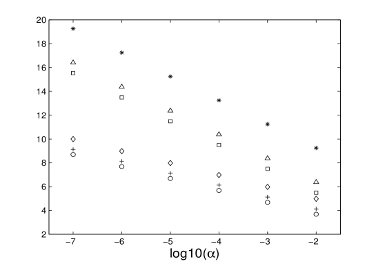
Figure 1: $log_{10}(\kappa^{\text{rel}}_{g}(A,b))$ (${+}$), $log_{10}(\underline{\kappa}^{\text{rel}}_{2})$ ($\circ$), $log_{10}(\bar{\kappa}^{\text{rel}}_{2})$ ($\diamond$), $log_{10}(\bar{\kappa}^{\text{rel}}_{1})$ ($\Box$), $log_{10}(\bar{\kappa}^{\text{rel}}(A,b))$ $(\Delta)$ and $log_{10}(\kappa^{\rm rel}_{TLS}(A,b))$ (${*}$) for $(m,n)=(500,350)$.

Example 3. Keep in mind that the distance between $\sigma_{n+1}$ and $\hat{\sigma}_{n}$ can control the conditioning of the TLS problem; see Theorems 8–9 or (78) and (79). In this example, we compare the bounds $\underline{\kappa}^{\text{rel}}_{2}$, $\bar{\kappa}^{\text{rel}}_{2}$, $\bar{\kappa}^{\text{rel}}_{1}$, $\kappa^{\rm rel}_{TLS}(A,b)$ and $\bar{\kappa}^{\rm rel}(A,b)$ for various distances between $\sigma_{n+1}$ and $\hat{\sigma}_{n}$. On the other hand, keep (61) in mind. Lemma 4.3 in [6] gives

$$\frac{|\hat{u}^{T}_{n}b|}{2\|x_{TLS}\|}\leq\hat{\sigma}_{n}-\sigma_{n+1}\leq\frac{\|b\|}{\|x_{TLS}\|},$$ (80)

which tells us that a small $\alpha$ implies that $\hat{\sigma}_{n}$ and $\sigma_{n+1}$ are close in some sense. In view of it, for given $m,n$, we construct $A\in\mathbb{R}^{m\times n}$ and $b\in\mathbb{R}^{n}$ with different distances between $\sigma_{n+1}$ and $\hat{\sigma}_{n}$ by taking different values of $\alpha$.

To do this, we first generate two $n\times n$ random orthogonal matrices $\bar{U}$ and $\bar{V}$ in the standard normal distribution. Then we take $\alpha=10^{-2},10^{-3},\ldots,10^{-7}$ and run the following function

$$V={\text{{{generator}}}}(n,\alpha,\bar{U},\bar{V})$$

$$u=\bar{U}(:,n);$$

$$vt=\bar{V}(:,n)^{\prime};$$

$$V_{11}=\bar{U}(:,1:n-1)*\bar{V}(:,1:n-1)^{\prime}+\alpha*u*vt;$$

$$t={\text{sqrt}}(1-\alpha*\alpha);$$

$$V=\left[~{}[V_{11},t*u];[t*vt,-\alpha]~{}\right];$$

respectively. In such a way, we get six orthogonal matrices $V\in\mathbb{R}^{(n+1)\times(n+1)}$ with $V(n+1,n+1)=-\alpha$ and $\alpha=10^{-2},10^{-3},\ldots,10^{-7}$, respectively. The idea of construction comes from Proposition 1. We generate randomly one $m\times(n+1)$ matrix $C_{1}$, and compute $C_{1}=U\Sigma V_{1}^{T}$ , the thin SVD of $C_{1}$. With the matrices $U$ and $\Sigma$ unchanged, we construct six matrices $C=U\Sigma V^{T}$ by replacing $V_{1}$ by the six orthogonal matrices $V$’s generated above. Set $A=C(:,1:n)$, $b=C(:,n+1)$, respectively. Then we get six different TLS problems. For each of them, $[A,\,b]=U\Sigma V^{T}$ is the thin SVD of $[A,\,b]$ and $V(n+1,n+1)=-\alpha$, where $\alpha=10^{-2},10^{-3},\ldots,10^{-7}$, respectively.

In such a way, with $(m,n)=(500,350)$ and $(1000,750)$, we generate $100$ samples for each $\alpha$, respectively. For each set of TLS problems with the same $\alpha$, we compute $\kappa^{\text{rel}}_{g}(A,b)$, $\underline{\kappa}^{\text{rel}}_{2}$, $\bar{\kappa}^{\text{rel}}_{2}$, $\bar{\kappa}^{\text{rel}}_{1}$, $\kappa^{\rm rel}_{TLS}(A,b)$ and $\bar{\kappa}^{\rm rel}(A,b)$. We plot the ($\log$ scale) averages of these quantities and the corresponding (log scale) $\alpha$ in Figures 1–2. We also report the averages of $1-\frac{\sigma_{n+1}}{\hat{\sigma}_{n}}$, a measure of the distance between $\sigma_{n+1}$ and $\hat{\sigma}_{n}$, in Table 5. We comment that the averages of $\frac{\sigma_{n+1}}{\sigma_{n}}$ for $(m,n)=(500,350)$ and $(1000,750)$ are $0.943$ and $0.958$, respectively.

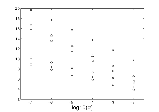
Figure 2: $log_{10}(\kappa^{\text{rel}}_{g}(A,b))$ ($+$), $log_{10}(\underline{\kappa}^{\text{rel}}_{2})$ ($\circ$), $log_{10}(\bar{\kappa}^{\text{rel}}_{2})$ ($\diamond$), $log_{10}(\bar{\kappa}^{\text{rel}}_{1})$ ($\Box$), $log_{10}(\bar{\kappa}^{\text{rel}}(A,b))$ $(\Delta)$ and $log_{10}(\kappa^{\rm rel}_{TLS}(A,b))$ (${*}$) for $(m,n)=(1000,750)$.

${(m,n)=(500,350)}$
$\alpha$	$~{}10^{-2}~{}$	$~{}10^{-3}~{}$	$~{}10^{-4}~{}$	$~{}10^{-5}~{}$	$~{}10^{-6}~{}$	$~{}10^{-7}~{}$
$1-\frac{\sigma_{n+1}}{\hat{\sigma}_{n}}$	$2.91\times 10^{-4}$	$2.92\times 10^{-6}$	$2.92\times 10^{-8}$	$2.92\times 10^{-10}$	$2.92\times 10^{-12}$	$2.88\times 10^{-14}$
${(m,n)=(1000,750)}$
$\alpha$	$10^{-2}$	$10^{-3}$	$10^{-4}$	$10^{-5}$	$10^{-6}$	$10^{-7}$
$1-\frac{\sigma_{n+1}}{\hat{\sigma}_{n}}$	$3.65\times 10^{-4}$	$3.66\times 10^{-6}$	$3.66\times 10^{-8}$	$3.66\times 10^{-10}$	$3.66\times 10^{-12}$	$3.52\times 10^{-14}$

Table 5: Example 3

We can see from Figures 1–2 and Table 5 that as $\alpha$ decreases, $\hat{\sigma}_{n}$ and $\sigma_{n+1}$ become closer, and the TLS problem becomes worse conditioned. $\kappa^{\rm rel}_{TLS}(A,b)$ always severely overestimates $\kappa^{\rm rel}_{g}(A,b)$. For $\alpha=10^{-2}$ in which $\hat{\sigma}_{n}$ and $\sigma_{n+1}$ are not very close, $\bar{\kappa}^{\rm rel}_{1}$ is tight and estimate $\kappa^{\rm rel}_{g}(A,b)$ accurately. For $\alpha=10^{-3}$, $\hat{\sigma}_{n}$ and $\sigma_{n+1}$ are closer. In this case, $\bar{\kappa}^{\rm rel}_{1}$ is no longer tight and estimate $\kappa^{\rm rel}_{g}(A,b)$ poorly but it still improves $\kappa^{\rm rel}_{TLS}(A,b)$ and $\bar{\kappa}^{\rm rel}(A,b)$ by about four orders and one order, respectively. We observe from Figures 1–2 that $\bar{\kappa}^{\rm rel}_{1}$, $\kappa^{\rm rel}_{TLS}(A,b)$ and $\bar{\kappa}^{\rm rel}(A,b)$ estimate $\kappa^{\rm rel}_{g}(A,b)$ more poorly as $\alpha$ decreases. Even so, $\bar{\kappa}^{\rm rel}_{1}$ is always smaller than $\kappa^{\rm rel}_{TLS}(A,b)$ and $\bar{\kappa}^{\rm rel}(A,b)$ by about four orders and one order, respectively. Remarkably, for all the cases, since ${\sigma}_{n}$ and $\sigma_{n+1}$ are not so close, $\underline{\kappa}^{\rm rel}_{2}$ and $\bar{\kappa}^{\rm rel}_{2}$ always estimate $\kappa^{\rm rel}_{g}(A,b)$ accurately.

$(m,n)$	$\kappa^{\text{rel}}_{g}(A,b)$	$\underline{\kappa}^{\text{rel}}_{2}$	$\bar{\kappa}^{\text{rel}}_{2}$	$\bar{\kappa}^{\text{rel}}_{1}$	$\bar{\kappa}^{\text{rel}}(A,b)$	$\kappa^{\rm rel}_{TLS}(A,b)$
$~{}(200,75)~{}$	$~{}1.46\times 10^{3}~{}$	$~{}5.59\times 10^{2}~{}$	$~{}8.58\times 10^{3}~{}$	$~{}3.19\times 10^{5}~{}$	$~{}1.01\times 10^{6}~{}$	$~{}2.48\times 10^{8}~{}$
$~{}(500,350)~{}$	$9.16\times 10^{3}$	$3.46\times 10^{3}$	$7.22\times 10^{4}$	$1.23\times 10^{6}$	$9.45\times 10^{6}$	$8.16\times 10^{9}$
$~{}(1000,75)~{}$	$3.14\times 10^{3}$	$6.19\times 10^{2}$	$2.22\times 10^{4}$	$2.57\times 10^{5}$	$3.58\times 10^{5}$	$2.13\times 10^{9}$
$~{}(1000,750)~{}$	$9.73\times 10^{4}$	$3.13\times 10^{4}$	$6.41\times 10^{5}$	$3.25\times 10^{8}$	$3.15\times 10^{9}$	$1.10\times 10^{12}$

Table 6: Example 4

Example 4. In this example, we generate the entries of $A$ and $b$ as random variables normally distributed with mean zero and variance one and observe $\underline{\kappa}^{\text{rel}}_{2}$, $\bar{\kappa}^{\text{rel}}_{2}$, $\bar{\kappa}^{\text{rel}}_{1}$, $\kappa^{\rm rel}_{TLS}(A,b)$ and $\bar{\kappa}^{\rm rel}(A,b)$. For each $(m,n)$, we conducted 100 random experiments. We report the average results of 100 experiments in Table 6. We observe that, as estimates of $\kappa^{\text{rel}}_{g}(A,b)$, both $\underline{\kappa}^{\text{rel}}_{2}$ and $\bar{\kappa}^{\text{rel}}_{2}$ are tight. The upper bound $\bar{\kappa}^{\text{rel}}_{2}$ improves $\bar{\kappa}^{\text{rel}}_{1}$ by one to two orders and improves $\kappa^{\rm rel}_{TLS}(A,b)$ and $\bar{\kappa}^{\rm rel}(A,b)$ by about five orders and one to four orders, respectively. $\bar{\kappa}_{1}^{\rm rel}$ is always smaller than $\bar{\kappa}^{\rm rel}(A,b)$. Clearly, the test TLS problems are quite well conditioned, but $\kappa^{\rm rel}_{TLS}(A,b)$ is a rather poor upper bound and overestimate $\kappa^{\rm rel}_{g}(A,b)$ too much.

7 Concluding Remarks

In the paper, we have studied the SVD-based condition number theory of the TLS problem. For the TLS condition number, we have established a new closed formula. Starting with it, we have derived sharp lower and upper bounds. Importantly and more practically, we have presented both lower and upper bounds that use only the smallest two singular values of $A$ and $[A,\ b]$. Numerical experiments have demonstrated the tightness of our bounds and the improvements of them over the two upper bounds in [1, 6]. Throughout the paper, the considered TLS problem is assumed to satisfy condition (2) and has a unique TLS solution. It is significant and important to extend the results presented in the paper to a general generic TLS problem [20, 21] that has non-unique TLS solutions or to the non-generic TLS problem [20]. We will consider these problems in forthcoming papers. Besides, it might be worthwhile to investigate how to apply the core problem theory [18] to study the TLS condition number.

Acknowledgements

The authors wish to thank the anonymous referees and the editor Professor Lothar Reichel for their suggestions and comments, which made us improve the presentation of the paper.

References

[1]
M. Baboulin, S. Gratton, A contribution to the conditioning of
the total least squares problem, SIAM J. Matrix Anal. Appl., 32 (2011)
685–699.
[2]
Å. Björck, Numerical Methods For Least Squares
Problems, SIAM, Philadelphia, PA, 1996.
[3]
Å. Björck, P. Heggernes, P. Matstoms, Methods for large
scale total least squares problems, SIAM J. Matrix Anal. Appl., 22
(2000) 413–429.
[4]
R. D. Fierro, J. R. Bunch, Perturbation theory for orthogonal
projection methods with applications to least squares and total
least squares, Linear Algebra Appl., 234 (1996) 71–96.
[5]
I. Gohberg, I. Koltracht, Mixed, componentwise, and structured
condition numbers, SIAM J. Matrix. Anal. Appl., 14 (1993) 688–704.
[6]
G. H. Golub, C. F. Van Loan, An analysis of the total least
squares problem, SIAM J. Numer. Anal., 17 (1980) 883–893.
[7]
G. H. Golub, C. F. Van Loan, Matrix Computations, 3rd Edition, Johns
Hopkins University Press, Baltimore, MD, 1996.
[8]
A. Graham, Kronecker Products and Matrix Calculus with Application,
Wiley, New York, 1981.
[9]
I. Hntynkov, M. Pleinger,
D. Maria Sima, Z. Strako, S. Van Huffel,
The total least squares problem in : A new
classification with the relationship to the classical works,
SIAM J. Matrix. Anal. Appl., 32 (2011) 748–770.
[10]
R. A. Horn, C. R. Johnson, Matrix Analysis, Cambridge
University Press, New York, 1985.
[11] Z. Jia, D. Niu, An implicitly restarted refined
bidiagonalization Lanczos method for computing a partial singular value
decomposition, SIAM J. Matrix Anal. Appl., 25 (2003) 246–265.
[12] Z. Jia, D. Niu, A refined harmonic Lanczos
bidiagonalization method and an implicitly restarted algorithm for
computing the smallest singular triplets of large matrices,
SIAM J. Sci. Comput., 32 (2010) 714–744.
[13]
J. Kamm, J. G. Nagy, A total least squares method for
Toeplitz system of equations, BIT, 38 (1998) 560–582.
[14]
B. Li, Z. Jia, Some results on condition numbers of the scaled
total least squares problem, Linear Algebra Appl., 435 (2011) 674–686.
[15]
X. Liu, On the solvability and perturbation analysis for total
least squares problem, Acta Mathematicae Applicatae Sinica, 19
(1996) 253–262 (in Chinese).
[16]
A. N. Malyshev, A unified theory of conditioning for linear
least squares and Tikhonov regularization solutions, SIAM J.
Matrix. Anal. Appl., 24 (2003) 1186–1196.
[17]
C. C. Paige, Z. Strako, Scaled total least squares
fundamentals, Numer. Math., 91 (2002) 117–146.
[18]
C. C. Paige, Z. Strako, Core problems in linear algebraic systems,
SIAM J. Matrix. Anal. Appl., 27 (2006) 861–875.
[19]
J. R. Rice, A theory of condition, SIAM J. Numer. Anal., 3
(1966) 287–310.
[20]
S. Van Huffel, J. Vandewalle, The Total Least Squares Problem:
Computational Aspects and Analysis, SIAM, Philadelphia, PA, 1991.
[21]
M. Wei, The analysis for the total least squares problem with
more than one solution, SIAM J. Matrix. Anal. Appl., 13 (1992)
746–763.
[22]
L. Zhou, L. Lin, Y. Wei, S. Qiao, Perturbation analysis and
condition numbers of scaled total least squares problems, Numer.
Algor., 51 (2009) 381–399.