Isospectral graphs with identical nodal counts

Abstract

According to a recent conjecture, isospectral objects have different nodal count sequences [20]. We study generalized Laplacians on discrete graphs, and use them to construct the first non-trivial counter-examples to this conjecture.
In addition, these examples demonstrate a surprising connection between isospectral discrete and quantum graphs.

1 Introduction

Nodal structures on continuous manifolds have been investigated ever since the days of Chladni. His work was experimental and involved the observation of nodal lines on vibrating plates. His research was resumed on a more rigorous footing by the pioneering works of Sturm [1, 2, 3], Courant [4] and Pleijel [5].
In recent years a surge of research has begun on inverse nodal problems, i.e. learning about the geometry of a system by observing its nodal features [16, 17, 18, 19, 25]. This research follows what is already known for many years in the regime of inverse spectral problems: one can deduce geometrical information about a system by observing its spectrum.
A key question in the framework of inverse spectral theory was posed by Mark Kac who asked (1966):“can one hear the shape of a drum?” [6]. Generally speaking, this question raises the issue of whether this information is unique. In other words, are there non-congruent systems with the exact same spectrum? (these are called isospectral systems). It turns out that the answer to this question is positive. Milnor was the first to show that there are isospectral systems in the case of flat tori in 16 dimensions [7]. After him we should mark a few names who contributed significantly to the study of the subject: Sunada [8] (Riemannian manifolds), Gordon ,Webb and Wolpert [9] as well as Buser et al. [10] (domains in $\mathbb{R}^{2}$), Band et al. [11] (quantum graphs) and Godsil and McKay [12] as well as Brooks [13] (discrete graphs).
As a matter of fact, in the context of graphs, Günthard and Primas [14] preceded Kac, raising the same question regarding the spectra of graphs with relation to Hückel’s theory (1956). A year later Collatz and Sinogowitz presented the first pair of isospectral trees [15].

As mentioned, aside from the spectrum, one can also try to mine information from the eigenfunctions of a given system. Today, it is known that there exists geometrical information in the nodal structures and nodal domains of eigenfunctions of manifolds, billiards and graphs [16, 17, 18, 19]. Furthermore, it is known that this geometrical information is different from the information one can deduce solely by observing the spectrum. The pioneering work began with Gnutzmann et al. [20, 21], and continued with many other papers, such as [22] for example.

In particular, Gnutzmann et al. [20] conjectured that isospectral systems could be differentiated by their nodal domain counts (we shall refer to it simply as the ‘conjecture’ throughout the paper). This conjecture has proven to be quite a strong one with many numerical and analytical evidence to back it up. In particular, in the case of graphs, both quantum and discrete there exist much numerical evidence as well as rigorous proofs for the validity of the aforementioned conjecture, see for example [23, 24, 25]. In addition, the conjecture was proven to hold for a family of isospectral four dimensional tori [22]. However, it was found recently that for a different method of counting, there exist a family of isospectral pairs of flat tori, sharing the same nodal domain counts [26]. This serves as a first counter-example to the conjecture.

In this paper, we would like to focus on the conjecture within the context of discrete graphs. We shall first demonstrate its strength and present some known results. Our main topic, however, is to display the first counter-example to the conjecture. To this end we will need to broaden our view from the usual operators defined on graphs, to the more general setting of weighted graphs.

In addition we would like to report a peculiarity which involves the discrete graphs of the counter-example. It turns out that this pair of isospectral (discrete) graphs are also isospectral as quantum graphs. This is intriguing since we have not been able to underatsnd this phenomena, nor could we build this isospectral pair using any of the (many) known methods which produce isospectral quantum graphs.

1.1 Discrete nodal domain theorems

Sturm [1, 2, 3], and Courant [4] after him, were the first to give analytical results about nodal domain counts on continuous systems. Denoting the nodal count sequence by $\{\nu_{n}\}$, Courant’s nodal domain theorem can be generally phrased as $\nu_{n}\leq n$.
In 1950 Gantmacher and Krein [27] investigated the sign patterns of eigenvectors of tridiagonal graphs, and in the 1970’s Fiedler wrote a couple of papers about the sign pattern of eigenvectors of acyclic matrices (matrices which are defined on trees) [28, 29]. Both Gantmacher and Krein, as well as Fiedler did not formulate their findings in the language of nodal domains. It took almost thirty years for the discrete counterpart of the Courant nodal domain theorem to appear. Gladwell et al. [30] and Davies et al. [31] were the first to discover this analogue, and soon afterwards they were followed by Biyikoglu [32] (who formulated a nodal domain theorem for trees). Recently a lower bound for the nodal count was derived by Berkolaiko [33]. This bound is given explicitly by $n-l\leq\nu_{n}$, where $l$ is the number of independent cycles of the graph.

Trees are an extremal class of graphs in the sense that for a given number of vertices, they are the smallest connected graph (least number of edges). For trees, assuming some generic conditions (which are manifested by the fact that the eigenvectors do not vanish on any of the vertices), it was proven that the nodal domain count of the $n^{th}$ eigenvector of the Laplacian matrix has exactly $n$ nodal domains [32, 33]. Therefore all trees (with the same number of vertices) share the same nodal domain count sequence. Furthermore, it is known that almost all tree graphs are isospectral [34] (meaning that almost any tree has a isospectral mate). This means that we cannot resolve the isospectrality using nodal domain counts, when it comes to trees. This shortcoming of the conjecture is well known, and to the best of our knowledge, occurs only for trees.
If we introduce weighted graphs, then there exist two more trivial counter-examples: complete graphs and polygon graphs (connected graphs in which all vertices have degree 2). In the case of complete weighted graphs, the first eigenvector has only one nodal domain and all other eigenvectors have exactly 2 nodal domains. Hence, they are an obvious counter-example. It should be noted that complete graphs are also extremal in the sense that for a given number of vertices, they are the largest connected graph (largest number of edges). For polygons, it can be shown (using the Courant bound [4] and Berkolaiko’s bound [33]) that polygons always have the same nodal count.

As far as the authors know, these three cases are the only counter-examples to the conjecture.

Aside from this extreme cases, in all isospectral graph pairs which were compared (analytically and numerically), different nodal domain sequences were observed [49]. In addition we have a proof for the conjecture for a certain class of discrete graphs [24].

Up until now, we only discussed isospectrality of the traditional matrices defined on graphs, most notably the adjacency matrix and the Laplacian. Additional work was done on less studied matrices such as the signless Laplacian and the normalized Laplacian.
However, since nodal domain theorems were proven for a more general class of matrices (generalized Laplacians), it is natural to test the conjecture for this class as well.

The paper is organized as follows. We will begin with some background and necessary definitions. The following section will describe the method of construction of isospectral weighted graphs. Then we will present the counter-example to the conjecture and finally prove the isospectrality of the quantum analogue of our discrete graphs.

2 Definitions

2.1 Discrete graphs

A graph $G$ is a set $\mathcal{V}$ of vertices connected by a set $\mathcal{E}$ of edges. The number of vertices is denoted by $V=|\mathcal{V}|$ and the number of edges is $E=|\mathcal{E}|$. The degree (valency) of a vertex is the number of edges which are connected to it. The number of independent cycles of a graph is denoted by $l$ and is given by $l=E-V+C$, where $C$ is the number of connected components of the graph.

The weighted adjacency matrix (connectivity) of $G$ is the symmetric $V\times V$ matrix $A=A(G)$ whose entries are given by:

$$A_{ij}=\left\{\begin{array}[]{ll}w_{ij},&\textrm{if $i$ and $j$ are adjacent}\\ 0,&\textrm{otherwise}\end{array}\right.$$

The $w_{ij}$’s values are called weights and are usually taken to be positive. For non-weighted graphs, all the weights are equal to unity. A diagonal element in $A$ corresponds to a loop, which is an edge connecting a vertex to itself. We shall only discuss graphs without loops.

A generalized Laplacian, $L(G)$, also known as a Schrödinger operator of $G$, is a matrix

$$L_{ij}=\left\{\begin{array}[]{ll}-w_{ij},&\textrm{if $i$ and $j$ are adjacent}\\ P_{i},&\textrm{if $i=j$}\\ 0,&\textrm{otherwise}\end{array}\right.$$

where $P_{i}$ is an arbitrary on-site potential which can assume any real value and $w_{ij}>0$. The combinatorial Laplacian results by taking all weights to be unity, and $P_{i}=-\sum_{j}w_{ij}=-deg(i)$, where $deg(i)$ is the degree of the vertex $i$. This way, the sum of each row, or column is equal to zero.
The eigenvalues of $L(G)$ together with their multiplicities, are known as the spectrum of $G$. To the $n^{th}$ eigenvalue, $\lambda_{n}$, corresponds (at least one) eigenvector whose entries are labeled by the vertex indices, i.e., $\phi_{n}=(\phi_{n}(1),\phi_{n}(2),\ldots,\phi_{n}(V))$. A nodal domain is a maximally connected subgraph of $G$ such that all vertices have the same sign with respect to $\phi_{n}$. The number of nodal domains of an eigenvector $\phi_{n}$ is called a nodal domain count, and will be denoted by $\nu_{n}$. The nodal count sequence of a graph is the number of nodal domains of eigenvectors of the Laplacian, arranged by increasing eigenvalues. This sequence will be denoted by $\{\nu_{n}\}_{n=1}^{V}$.
We recall that the known bounds for the nodal count [30, 31, 33] are

$$n-l\leq\nu_{n}\leq n.$$ (1)

2.2 Quantum graphs

To define quantum graphs a metric is associated to $G$. That is, each edge is assigned a positive length: $L_{e}\in(0,\infty)$. The total length of the graph will be denoted by $\mathcal{L}=\sum_{e\in\mathcal{E}}L_{E}$. This enables to define the metric Laplacian (or Schrödinger) operator on the graph as the Laplacian in 1-d $-\frac{{\rm d}^{2}\ }{{\rm d}x^{2}}$ on each bond. The domain of the Schrödinger operator on the graph is the space of functions which belong to the Sobolev space $H^{2}(e)$ on each edge $e$ and satisfy certain vertex conditions. These vertex conditions involve vertex values of functions and their derivatives, and they are imposed to render the operator self adjoint. We shall consider in this paper only the so-called Neumann vertex conditions:

$${\rm Neumann}\ \ \ \ \forall v\ \ :\ \ \ \sum_{e\in S^{(v)}}\left.\frac{{\rm d}\ \ \ }{{\rm d}x_{e}}\ \psi_{e}(x_{e})\right|_{x_{e}=0}\ =\ 0\ \$$ (2)

where $S^{(v)}$ is the set of all edges connected to the vertex $v$. The derivatives in (2) are directed out of the vertex $v$. The eigenfunctions are the solutions of the edge Schrödinger equations:

$$\ \ \forall e\in E\ \ -\frac{{\rm d}^{2}\ }{{\rm d}x^{2}}\psi_{e}=k^{2}\psi_{e},$$ (3)

which satisfy at each vertex the Neumann conditions (2). The spectrum $\{k_{n}^{2}\}_{n=1}^{\infty}$ is discrete, non-negative and unbounded. One can generalize the Schrödinger operator by including potential and magnetic flux defined on the bonds. Other forms of vertex conditions can also be used. However, these generalizations will not be addressed here, and the interested reader is referred to two recent reviews [35, 36].

Finally, Two graphs, $G_{1}$ and $G_{2}$, are said to be isospectral if they posses the same spectrum (same eigenvalues with the same multiplicities). In perfect analogy, two graphs with the same nodal domain sequence will be referred to as isonodal. These two definitions hold both for discrete and quantum graphs.

3 Isospectrality and isonodality

3.1 Isospectral graphs construction

Our method for constructing isospectral graphs is a variation of a method described in [38], called the line graph construction. This method uses the gallery of isospectral billiards of Buser et al. [10] in order to build isopectral discrete graphs. A similar idea was used by Gutkin et al. [37] to construct isospectral discrete and quantum graphs.
A line graph is built from a “parent” graph in the following way: each edge becomes a vertex, and two vertices in the line graph are adjacent if and only if their corresponding edges shared a vertex in the parent graph. In [38] an example is given, based on the first family of isospectral domains in [10] called the $7_{1}$ family. Our method is simpler than the one in [38]. It results with graphs with the same topology as in [38], but with different Laplacian matrices.

Instead of using the gallery of billiards as it appears in [10], we use a graph representation of them as it is described in [39]. In particular, the $7_{1}$ family is shown in figure 1.

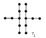
Figure 1: The $7_{1}$ family in the representation presented in [39].

We consider the two graphs in figure 1 as parent graphs and apply the line graph construction on them. We still have to specify how we assign weights in the resulting line graphs. We start by assigning three different weights: $a,b,c>0$ to each of the three types of edges in the parent graphs. Suppose that in the parent graph, an edge of weight $a$ shared a vertex with an edge of weight $b$ ($a\neq b$). Then, in the line graph, the corresponding vertices would be connected by an edge of the remaining weight $c\neq a,b$.
The two resulting weighted line graphs are shown in figure 2. Let us denote the left graph by $G_{1}$ and the right one by $G_{2}$.

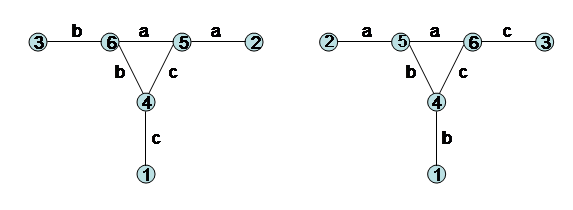
Figure 2: Two isospectral graphs constructed through the line graph construction from the $7_{1}$ billiards.

The generalized Laplacians of the two graphs are given explicitly by following matrices:

$$L_{1}=-\left(\begin{array}[]{cccccc}0&0&0&c&0&0\\ 0&0&0&0&a&0\\ 0&0&0&0&0&b\\ c&0&0&0&c&b\\ 0&a&0&c&0&a\\ 0&0&b&b&a&0\\ \end{array}\right)L_{2}=-\left(\begin{array}[]{cccccc}0&0&0&b&0&0\\ 0&0&0&0&a&0\\ 0&0&0&0&0&c\\ b&0&0&0&b&c\\ 0&a&0&b&0&a\\ 0&0&c&c&a&0\\ \end{array}\right)$$ (16)

It is not hard to check that for any $a,b,c$, the characteristic polynomials of $L_{1}$ and $L_{2}$ are identical and hence the graphs are isospectral. Another way to prove the isospectrality is to construct the transplantation matrix $T$ such that $T^{-1}L_{1}T=L_{2}$. Then it is clear that the two matrices are similar and therefore isospectral. The transplantation matrix between $L_{1}$ and $L_{2}$ is

$$T=\left(\begin{array}[]{cccccc}0&-1&0&0&0&1\\ -1&0&0&0&1&0\\ 0&0&-1&1&0&0\\ 0&0&1&1&0&0\\ 0&1&0&0&0&1\\ 1&0&0&0&1&0\\ \end{array}\right)$$ (17)

The same construction can be carried out for any graph in the gallery of [39].
We can construct many more isospectral graphs by using polynomials in $L_{1}$ and $L_{2}$. Namely, for any polynomial $P$, we will consider $P(L_{1})$ and $P(L_{2})$ as the Laplacian matrices of two new weighted graphs (assuming that $P(L_{1})$ and $P(L_{2})$ are indeed generalized Laplacians as defined in section 2.1). These two graphs might be topologically different than the original $G_{1}$ and $G_{2}$. Since we have a transplantation matrix, it is clear that $P(L_{1})$ and $P(L_{2})$ are similar matrices and therefore the resulting graphs are also isospectral.

3.2 Failure of the conjecture regarding nodal domain counts

We have introduced the conjecture that the isospectrality between graphs can be resolved by counting nodal domains. We have also said that three known cases (trees, polygons and complete graphs) are exceptions to this conjecture. We now prove that $G_{1}$ and $G_{2}$ cannot be resolved by counting nodal domains. This is a non-trivial exception to the conjecture.

We define the vertices with degree larger than one as the interior vertices (vertices $4,5,6$), and the rest as boundary vertices (vertices $1,2,3$).
We begin by checking the relations between the interior and boundary vertices.
Let $\phi_{n}^{1}$ be the $n^{th}$ eigenfunction of $L_{1}$, and $\phi_{n}^{2}$ be the $n^{th}$ eigenfunction of $L_{2}$. For the first graph, we get the following relations:

$$\phi_{n}^{1}(1)=\frac{-c}{\lambda_{i}}\phi_{n}^{1}(4)\\ \phi_{n}^{1}(2)=\frac{-a}{\lambda_{i}}\phi_{n}^{1}(5)\\ \phi_{n}^{1}(3)=\frac{-b}{\lambda_{i}}\phi_{n}^{1}(6)$$ (18)

For the second graph, we get the same relations with $b$ and $c$ replaced. Therefore, since the weights are positive, if $\lambda_{n}<0$ then each boundary vertex has the same sign as the interior vertex connected to it. This means that for $\lambda_{n}<0$, the boundary vertices will not contribute to the nodal domain count. On the other hand, if $\lambda_{n}>0$, each boundary vertex has an opposite sign than the interior vertex connected to it. This means that for $\lambda_{n}>0$, the boundary vertices will contribute three to the nodal domain count. The most important point is that the contribution of the boundary vertices to the nodal count depends on the spectrum, and since the two graphs are isospectral, it is the same for both graphs. As a result, it is enough to compare only the nodal count sequence of the interior vertices.
The interior vertices form a triangle. Therefore the nodal domain count of any vector, on the subgraph induced by the interior vertices, is either one or two. By computing the rest of the equations, and with the aid of (18), we can formulate the conditions for having one or two nodal domains.
The interior nodal domain count of a vector $\phi_{i}$ (of any of the graphs) is one if and only if one of the following is true:

$$\{\lambda_{n}<0\ \textrm{and}\ \left|\lambda_{n}\right|>\max{(a,b,c)}\}\ \textrm{or}$$

$$\{\lambda_{n}>0\ \textrm{and}\ \lambda_{n}<\min{(a,b,c)}\}.$$ (19)

In any other case, the nodal domain count is two.
In other words, a nodal domain count of a specific vector, is determined uniquely by the corresponding eigenvalue. Therefore, the entire nodal domain counts of the graphs are determined by the spectrum, and since the two graphs are isospectral, the nodal count sequence does not resolve the isospectrality.

As we have shown in subsection 3.1, for any polynomial $P$, the two graphs represented by $P(L_{1})$ and $P(L_{2})$ are isospectral. We will now show that these graphs are also isonodal, thus extending our family of counter-examples to the conjecture.
Assuming that the weights $a,b,c$ are rationally incommensurate, the following observations can be easily proven:

• If the polynomial consists only of a second degree term ($P(x)=cx^{2}$), then the obtained graphs $P(L_{1})$ and $P(L_{2})$ are given by figure 3.

• If $P(x)=c_{1}x+c_{2}x^{2}$, then the obtained graphs $P(L_{1})$ and $P(L_{2})$ are given by figure 4.

• Polynomials of third degree or larger represent weighted, complete graphs, which are trivial counter-examples to the conjecture (see section 1.1).

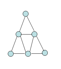
Figure 3: The graph obtained by applying a polynomial $P(x)=cx^{2}$.

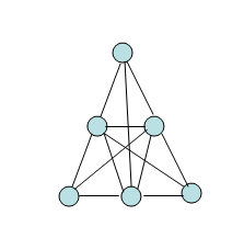
Figure 4: The graph obtained by applying a polynomial $P(x)=c_{1}x+c_{2}x^{2}$

For these reasons, we only need to check the first two cases above.
The resulting graphs, In both cases, clearly have the same eigenvectors as $G_{1}$ and $G_{2}$. Then, using (18) and (19), it can be easily shown that in both types of graphs, the nodal count is determined by the spectrum, precisely as is the case with $G_{1}$ and $G_{2}$.
We conclude that both types of graphs are isonodal and as a consequence, they are also non-trivial counter-examples to the conjecture.

Remark: Applying the line graph construction to other families from the gallery in Buser et al. [10], one can build many pairs of isospectral graphs. Some of these pairs are isonodal (such as the $7_{2}$ and $7_{3}$ families) and some are not (such as the $13_{2}$ family).

4 Isospectral quantum graphs

When we come to discuss quantum graphs, we need to define the lengths of the different edges. The weights we put on the weighted discrete graphs can be viewed as coupling constants. Thus, the most intuitive notion is to associate a length which is inversely proportional to the weights. If we also specify the vertex conditions, we go from the realm of discrete graphs into the realm of quantum graphs.
We then come to ask the following interesting question: is the isospectrality preserved when we enter the world of quantum graphs? This question is only a small part of a much broader subject - the spectral relations between quantum graphs and the underlying discrete graphs. This subject was addressed by several authors in the past, see for example [40, 41, 42, 43]. However, most of these references have a complete analysis only for equilateral quantum graphs, with Neumann vertex conditions. The graphs $G_{1}$ and $G_{2}$ are not equilateral, and therefore we cannot make an a-priori prediction whether or not the isospectrality is preserved.

Nevertheless, we will show by direct computation that $G_{1}$ and $G_{2}$ are indeed isospectral as quantum graphs, once Neumann vertex conditions are considered at all vertices.
A function $\psi$ on the graph, which is continuous on the vertices, can be written as:

$$\psi|_{(i,j)}=\frac{1}{\sin{kL_{ij}}}\left[\phi(i)\sin{k(L_{ij}-x)}+\phi(j)\sin{kx}\right],$$ (20)

where $\phi(i)$ is the value of the function on the vertex $i$ and $L_{ij}$ is the length of the edge $(i,j)$. Note, that we still use the notations $a,b,c$ to denote the lengths of the edges.

The Neumann vertex conditions on the boundary vertices for $G_{1}$, dictate these relations:

$$\phi(1)=\frac{\phi(4)}{\cos{kc}}\\ \phi(2)=\frac{\phi(5)}{\cos{ka}}\\ \phi(3)=\frac{\phi(6)}{\cos{kb}}$$ (21)

The Neumann conditions on the interior vertices are (we make use of (21)):

$$-\frac{1}{\sin{kc}}\left[-\frac{\phi(4)}{\cos{kc}}+\phi(4)\cos{kc}\right]+\frac{1}{\sin{kc}}\left[-\phi(4)\cos{kc}+\phi(5)\right]+\frac{1}{\sin{kb}}\left[-\phi(4)\cos{kb}+\phi(6)\right]=0$$ (22)

$$\frac{1}{\sin{ka}}\left[-\frac{\phi(5)}{\cos{ka}}+\phi(5)\cos{ka}\right]+\frac{1}{\sin{kc}}\left[\phi(5)\cos{kc}-\phi(4)\right]-\frac{1}{\sin{ka}}\left[-\phi(5)\cos{ka}+\phi(6)\right]=0$$ (23)

$$\frac{1}{\sin{kb}}\left[-\frac{\phi(6)}{\cos{kb}}+\phi(6)\cos{kb}\right]+\frac{1}{\sin{kb}}\left[\phi(6)\cos{kb}-\phi(4)\right]+\frac{1}{\sin{ka}}\left[\phi(6)\cos{ka}-\phi(5)\right]=0$$ (24)

This can be written more conveniently as a matrix-vector product:

$$A^{1}(k)\bm{\phi}=0$$ (25)

Where $1$ comes to represent that this is the matrix corresponding to $G_{1}$, and $\bm{\phi}=(\phi(4),\phi(5),\phi(6))$.
The matrix $A^{1}(k)$ is:

$$A^{1}(k)=\left(\begin{array}[]{ccc}2\cot{2kc}+\cot{kb}&\frac{-1}{sin{kc}}&\frac{-1}{sin{kb}}\\ \frac{-1}{sin{kc}}&2\cot{2ka}+\cot{kc}&\frac{-1}{sin{ka}}\\ \frac{-1}{sin{kb}}&\frac{-1}{sin{ka}}&2\cot{2kb}+\cot{ka}\\ \end{array}\right)$$

(25) has a solution if and only if

$$h^{1}(k)\equiv\det{A^{1}(k)}=0$$ (26)

$h^{1}(k)$ is called the secular function, and equation (26) is called the secular equation. It is fulfilled at the values $k$ which are in the spectrum of the Laplacian of the graph. We can get $A^{2}(k)$ by switching the lengths $b$ and $c$ in $A^{1}(k)$. It can be easily checked that $h^{1}(k)=h^{2}(k)\equiv h(k)$, hence the graphs are isospectral.

Although we have proven that $G_{1}$ and $G_{2}$ are isospectral as quantum graphs, the profound reason for this is still a riddle for us. The recent papers on isospectrality [11, 45] generalize former seminal papers such as those of Sunada [8] and Buser et al. [10], and can produce many of the known examples of isopectral quantum graphs. However, we were not able to build the two graphs $G_{1}$ and $G_{2}$ using the constructions described in [11, 45]. Furthermore, We were unable to build a transplantation matrix for the quantum graphs (although there is a transplantation matrix for the discrete case - see (17)). It should be emphasized that all isospectral quantum graphs which are built using any of the methods in [8, 10, 11, 45] posses a transplantation matrix between the two graphs. In [44], the authors consider the two graphs in the present paper and turn them into scattering systems. They prove that there is no transplantation which involves the values of the eigenfunctions on the vertices. They do not, however, eliminate the possibility of having any other form of transplantation. All these pieces of evidence suggest that $G_{1}$ and $G_{2}$ might belong to a new class of isospectral quantum graphs.

Remark: Unlike the graphs $G_{1}$ and $G_{2}$ which correspond the the $7_{1}$ family, the isospectrality is not preserved in the $7_{2}$ and $7_{3}$ graphs (i.e., the corresponding quantum graphs are not isospectral). This leads us to contemplate the issue of converting isospectral weighted discrete graphs into their isospectral quantum analogues. How to do so, or whether at all it is possible, remains an open problem.

5 Summary

The conjecture that isospectrality can be lifted by comparing nodal domain counts was originally stated for flat tori of dimension larger than three [20]. Later on, this conjecture was proven for four-dimensional flat tori [22]. However, using a different counting method, a family of both isosepctral and isonodal pairs of flat tori was discovered [26].

The conjecture was imported into the realm of graphs where it was proven for some quantum and discrete graphs [23, 24]. In addition, there exist much numerical evidence for the validity of the conjecture in discrete graphs [49] (using a construction by Godsil and McKay [12]).

In this paper we show that for discrete graphs, the conjecture is not true in its most general form. What we demonstrate is that if we use generalized Laplacians, the conjecture ceases to be valid even for graphs which are not extremal. One should keep in mind that if we restrict ourselves only to the traditional matrices - the adjacency and Laplacian matrices - then the only known counter-examples to the conjecture are trees.

The paper also presents an intriguing connection between isospectral discrete and quantum graphs. The fact that both the discrete graphs, and their quantum analogues are isospectral, calls for more study on the relation between these two regimes.

6 Acknowledgements

The authors warmly thank Uzy Smilansky for his continuous support, significant encouragement and for many invaluable discussions. The work was supported by ISF grant 169/09. RB is supported by EPSRC, grant number EP/H028803/1.

References

References

- [1] C. Sturm, M’moire sur les équations différentielles linéaires du second ordre, J. Math. Pures Appl., 1:106 186, 1836.
- [2] C. Sturm, M‘moire sur une classe d équations à différences partielles, J. Math. Pures Appl., 1:373 444, 1836.
- [3] D. Hinton, Sturm s 1836 oscillation results: evolution of the theory, In Sturm-Liouville theory, pages 1 27. Birkh user, Basel, 2005.
- [4] R. Courant and D. Hilbert, Methods of Mathematical Physics, Vol. 1, Interscience, New York, 1953.
- [5] A. Pleijel, Remarks on Courant’s nodal line theorem, Comm. Pure Appl. Math. 9, 543-550, 1956.
- [6] M. Kac, Can one hear the shape of a drum?, American Mathematical Monthly 73 (4, part 2), 1 23, 1966.
- [7] J. Milnor, Eigenvalues of the Laplace operator on certain manifolds, Proceedings of the National Academy of Sciences of the United States of America 51, 542ff, 1964.
- [8] T. Sunada, Riemannian coverings and isospectral manifolds, Ann. Of Math. (2) 121 (1), 169 186, 1985.
- [9] C. Gordon, D. Webb, S. Wolpert, One Cannot Hear the Shape of a Drum, Bulletin of the American Mathematical Society 27 (1), 134 138, 1992.
- [10] P. Buser, J. Conway, P. Doyle and K. D. Semmler, Some planar isospectral domains, International Mathematics Research Notices 9: 391ff’ 1994.
- [11] R. Band, O. Parzanchevski and G. Ben-Shach, The isospectral fruits of representation theory: quantum graphs and drums, J. Phys. A: Math. Theor. 42 175202, 2009.
- [12] C. D. Godsil and B. D. McKay, Constructing cospectral graphs, Aequationes Mathematicae 25, 257-268, 1982.
- [13] R. Brooks, Non-Sunada graphs, Ann. Inst. Fourier 49 707 25, 1999.
- [14] Hs. H. Gunthard and H. Primas, Zusammenhang von Graphentheorie und MO-Theorie von Molekeln mit Systemen konjugierter Bindungen, Helv. Chim. Acta 39, pp. 1645 1653, 1956.
- [15] L. Collatz and U. Sinogowitz, Spektren endlicher Grafen, Abh. Math. Sem. Univ. Hamburg. 21, pp. 63 77, 1957.
- [16] S. Gnutzmann, P.D. Karageorge, U. Smilansky, Can One Count the Shape of a drum?, Phys. Rev. Lett. 97, 090201 (2006).
- [17] S. Gnutzmann, P.D. Karageorge, U. Smilansky, A trace formula for the nodal count sequence – Towards counting the shape of separable drums, Eur. Phys. J. Special Topics 145, 217 (2007)
- [18] P.D. Karageorge, U. Smilansky, Counting nodal domains on surfaces of revolution, J. Phys. A 41, 205102 (2008).
- [19] D. Klawonn, Inverse Nodal Problems, J. Phys. A 42, 175209 (2009).
- [20] S. Gnutzmann, U. Smilansky and N. Sondergaard, Resolving isospectral ‘drums’ by counting nodal domains, J. Phys. A: Math. Gen. 38 8921 33, 2005.
- [21] S. Gnutzmann, P. D. Karageorge and U. Smilansky, Can One Count the Shape of a Drum?, Phys. Rev. Lett. 97 090201, 2006.
- [22] J. Brüning, D. Klawonn, and C. Puhle, Remarks on ”Resolving isospectral ‘drums’ by counting nodal domains”, J. Phys. A, 40(50):15143-15147, 2007.
- [23] R. Band, T. Shapira and U. Smilansky, Nodal domains on isospectral quantum graphs: the resolution of isospectrality?, J. Phys. A.: Math. Gen. 39 13999-4014, 2006.
- [24] I. Oren, Nodal domain counts and the chromatic number of graphs, J. Phys. A: Math. Theor. 40 9825, 2007.
- [25] R. Band, I. Oren, and U. Smilansky, Nodal domains on graphs - How to count them and why?, in [47].
- [26] J. Brüning, D. Fajman, On the nodal count for flat tori, to appear in Comm. Math. Phys., 2011.
- [27] F. R. Gantmacher and M. G. Krein, Oscillation Matrices and Kernels and Small Vibrations of Mechanical Systems, State Publishing House of Technical-Theoretical Literature, Moscow, Leningrad, 1950. English Translation by US Atomic Energy Commission, Washington D. C. 1961.
- [28] M. Fiedler, Eigenvectors of acyclic matrices, Czechoslovak Math. J., 25, 607-618, 1975.
- [29] M. Fiedler, A property of eigenvectors of non-negative symmetric matrices and its application to graph theory, Czechoslovak Math. J., 25, 619-633, 1975.
- [30] G. M. L. Gladwell and H. Zhu, Courant s nodal line theorem and its discrete counterparts’ Quart. J. Mech. Appl. Math., 55(1), 1 15, 2002.
- [31] E. B. Davies, G. M.L. Gladwell, J. Leydold and P. F. Stadler, Discrete Nodal Domain Theorems, Linear Algebra and its Applications Vol. 336, October, pp. 51-60, 2001.
- [32] T. Biyikolu, A discrete nodal domain theorem for trees, Linear Algebra Appl. 360, 197-205, 2003.
- [33] G. Berkolaiko, A lower bound for nodal count on discrete and metric graphs, Comm. Math. Phys., 278(3), 803 819, 2008.
- [34] A.J. Schwenk, Almost all trees are cospectral, In: New Directions in the Theory of Graphs, F. Harary, Editor, Academic Press, New York, pp. 275 307, 1973.
- [35] S. Gnutzmann and U. Smilansky, Quantum graphs: Applications to quantum chaos and universal spectral statistics, Advances in Physics, 55 (5-6), 527-625, 2006.
- [36] P. Kuchment, Quantum graphs: an introduction and a brief survey, In Analysis on graphs and its applications, volume 77 of Proc. Sympos. Pure Math., Amer. Math. Soc., Providence, RI, 291-312 , 2008.
- [37] B. Gutkin and U. Smilansky, Can one hear the shape of a graph?, J. Phys. A: Math. Gen. 31 6061 8, 2001.
- [38] P. McDonald and R. Meyers, Isospectral polygons, planar graphs and heat content, Proceedings of the American mathematical society, Vol. 131, Number 11, Pages 3589-3599 S 0002-9939(03)07123-5 Article electronically published on June 18, 2003.
- [39] Y. Okada and A. Shudo 2001 J. Phys. A: Math. Gen. 34 5911 22.
- [40] J. von Below, A Characteristic Equation Associated to an Eigenvalue Problem on -Networks, Linear Algebra and its Applications, 71: 309-325 (1985).
- [41] J. von Below, Can one hear the shape of a network?, in [48], 19-36, 2001.
- [42] C. Cattaneo, The spectrum of the continuous Laplacian on a graph, Monatsh. Math. 124 (1997), no. 3, 215 235.
- [43] O. Post, Equilateral quantum graphs and boundary triples, in [47].
- [44] R. Band, A. Sawicki and U. Smilansky, Scattering from isospectral quantum graphs, J. Phys. A: Math. Theor. 43 415201, 2010.
- [45] O. Parzanchevski and R. Band, Linear Representations and Isospectrality with Boundary Conditions, J. Geom. Anal. 20 439-71, 2010.
- [46] J.P Roth, Le spectre du Laplacien sur un graphe Th eorie du Potentiel Lect Not. Math. vol. 1096 (Berlin: Springer) 521-539, 1983.
- [47] P. Exner, J. P. Keating, P. Kuchment, T. Sunada, and A. Teplyaev (Editors), Analysis on Graphs and its Applications, Proc. Symp. Pure Math., AMS.
- [48] F.A. Mehmeti, J. von Below, and S. Nicaise (Editors), Partial differential equations on multistructures, Proceedings of the International Conference held in Luminy, April 19 24, 1999, Lecture Notes in Pure and Applied Mathematics, 219. Marcel Dekker, Inc., New York, 2001.
- [49] I. Oren and U. Smilansky, private communication.