Scalar Quantum Field Theory on Fractals

Arnab Kar111arnabkar@pas.rochester.edu  and S. G. Rajeev 222rajeev@pas.rochester.edu 333Also at the Department of Mathematics
Abstract

We construct a family of measures for random fields based on the iterated subdivision of simple geometric shapes (triangles, squares, tetrahedrons) into a finite number of similar shapes. The intent is to construct continuum limits of scale invariant scalar field theories, by imitating Wiener’s construction of the measure on the space of functions of one variable. These are Gaussian measures, except for one example of a non-Gaussian fixed point for the Ising model on a fractal. In the continuum limits what we construct have correlation functions that vary as a power of distance. In most cases this is a positive power (as for the Wiener measure) but we also find a few examples with negative exponent. In all cases the exponent is an irrational number, which depends on the particular subdivision scheme used. This suggests that the continuum limits corresponds to quantum field theories (random fields) on spaces of fractional dimension.

Department of Physics and Astronomy

University of Rochester

Rochester NY 14627

USA

1 Introduction

Wiener constructed a Gaussian measure on functions of one variable by subdividing the interval and imposing the scale invariance of the measure[1]. By subdividing the plane into triangles, and space into tetrahedrons, we construct analogous measures for functions of several variables. These are field theoretic analogues of the hierarchical models[2] commonly studied in spin systems[3]. They can also be viewed as the quantum analogues of the Laplace equation on fractals studied by Strichartz[4]. The method we use is to seek fixed points of the “real space renormalization group”, which has been in use in statistical physics for many years[5].

There are other approaches to constructing quantum field theories in fractional dimensions [6], in part motivated by the success of dimensional regularization. But our construction appears to be more direct, being based on a finite element method. It does not appear to be possible to construct scale invariant Gaussian measures of quantum field theories in integer space dimension greater than one by our method of iterating finite integrals. We extend our ideas of scale invariance to other systems like the Ising model, to find a non trivial unstable fixed point for a fractal of dimension greater than two. The critical exponents are calculated in this case using ideas of statistical mechanics.

In the continuum limit what we construct is a quantum field theory of fractional scaling dimension, with a correlation function that varies as a power of distance; this power is often positive, but we also find a few cases where it is negative. An example of a system with growing correlation function would be that of Brownian motion. The average distance two points undergoing Brownian motion increases with time as $<\left[x(t_{1})-x(t_{2})\right]^{2}>\sim|t_{1}-t_{2}|$.

Physicists denote the Wiener measure by

$$\int{\cal D}\phi e^{-\frac{1}{2}\int\phi^{\prime 2}dx}$$

Exactly what does this mean? There certainly is no Lebesgue measure which can be called $\mathcal{D}\phi$ in the space of functions because that space is infinite dimensional. Also, the functions $\phi$ are, with probability one under the Wiener measure, not differentiable. $\phi^{\prime}$ is at best a distribution. So it does not have a sensible product: $\phi^{\prime 2}$ is by itself meaningless.

Recall that the derivative $\frac{dy}{dx}$ in calculus is to be understood as a limit constructed using epsilons and deltas of modern analysis, and not as some infinitesimal divided by another. Similarly, the path integral is to be understood as a limit of finite dimensional integrals. The action being the integral of a local Lagrangian ( a function of the field and its derivative) is not to be taken literally. Indeed, a limit of a sequence of local measures (that depends only on nearest neighbors of the triangulation) may not tend even formally to a local action principle.

In order to construct the scale invariant measures in higher dimensions, the field variable could acquire an anomalous dimension. As a consequence, the correlation functions have irrational numbers as their scaling exponent. In the simplest examples, $G(x_{1},x_{2})=<[\phi(x_{1})-\phi(x_{2})]^{2}>$ scales as $|x_{1}-x_{2}|^{0.611516}$ for the subdivision of right angled triangled triangles and as $|x_{1}-x_{2}|^{0.329351}$ for tetrahedrons. These exponents are not universal as other subdivision methods lead to other exponents.We suggest that this exponent of the correlation function of the Gaussian be used as a measure of the dimension of a fractal, analogous to the Hausdorff dimension: it is more relevant for the behavior of randomness in quantum systems.

2 Subdividing the Real Line

Suppose that $\phi_{0}$ and $\phi_{1}$ are the boundary values of the field on the interval $[x_{0},x_{1}]$ of length $a=x_{1}-x_{0}.$ Integrating out the field everywhere on the inside of the interval induces some measure $h(\phi_{1},x_{1}|\phi_{0},x_{0})d\phi_{0}d\phi_{1}$ on the boundary values. The simplest possibility is a Gaussian that is translation invariant in field values

$$h(\phi_{1},x_{1}|\phi_{0},x_{0})=C_{a}e^{-\frac{1}{2}\alpha_{a}(\phi_{1}-\phi_{0})^{2}}$$

for some $\alpha_{a}$ and $C_{a}$ which can depend on $|x_{1}-x_{0}|$. If we subdivide the interval into two (for example, at its midpoint $x_{01}=\frac{1}{2}(x_{1}+x_{0})$) and integrate over the field at the new point, we should get back the original measure.

$$\int h(\phi_{1},x_{1}|\phi_{01},x_{01})h(\phi_{01},x_{01}|\phi_{0},x_{0})d\phi_{10}=h(\phi_{1},x_{1}|\phi_{0},x_{0})$$

This leads to the conditions

$\displaystyle C_{\frac{a}{2}}^{2}\int\exp\left\{-\frac{1}{2}\alpha_{\frac{a}{2}}\left[(\phi_{1}-\phi_{01})^{2}+(\phi_{01}-\phi_{0})^{2}\right]\right\}d\phi_{10}$ $\displaystyle=$ $\displaystyle C_{a}\exp\left\{-\frac{1}{2}\alpha_{a}(\phi_{1}-\phi_{0})^{2}\right\}$
$\displaystyle C_{a}$ $\displaystyle=$ $\displaystyle C_{\frac{a}{2}}^{2}$

By completing the square,

$$C_{\frac{a}{2}}^{2}\int\exp\left\{-\frac{1}{2}\alpha_{\frac{a}{2}}\left[2\left(\phi_{01}-\frac{\phi_{0}+\phi_{1}}{2}\right)^{2}\right]\right\}d\phi_{10}\exp\left\{-\frac{1}{2}\alpha_{\frac{a}{2}}\frac{(\phi_{1}-\phi_{0})^{2}}{2}\right\}=C_{a}\exp\left\{-\frac{1}{2}\alpha_{a}(\phi_{1}-\phi_{0})^{2}\right\}$$

Thus,

$\displaystyle\frac{1}{2}\alpha_{\frac{a}{2}}$ $\displaystyle=$ $\displaystyle\alpha_{a}$
$\displaystyle C_{\frac{a}{2}}^{2}\sqrt{\frac{\pi}{\alpha_{\frac{a}{2}}}}$ $\displaystyle=$ $\displaystyle C_{a}$

Solving

$\displaystyle\alpha_{a}$ $\displaystyle=$ $\displaystyle\frac{\alpha}{a}$
$\displaystyle C_{a}$ $\displaystyle=$ $\displaystyle\sqrt{\frac{\alpha}{2\pi a}}$
$\displaystyle h(\phi_{1},x_{1}|\phi_{0},x_{0})$ $\displaystyle=$ $\displaystyle\frac{\sqrt{\alpha}}{\sqrt{2\pi(x_{1}-x_{0})}}e^{-\frac{\alpha}{2(x_{1}-x_{0})}(\phi_{1}-\phi_{0})^{2}}$

By repeated subdivisions of the interval we would get the integral

$$\int\prod_{i}d\phi_{i}e^{-\frac{\alpha}{2}\sum_{i}\frac{(\phi_{i+1}-\phi_{i})^{2}}{x_{i+1}-x_{i}}}$$

In the limit of small size of the interval, the exponent can be interpreted as

$$\frac{\alpha}{2}\int\phi^{\prime 2}dx$$

justifying the physicists’ notation

$$\int\prod_{i}d\phi_{i}e^{-\frac{\alpha}{2}\sum_{i}\frac{(\phi_{i+1}-\phi_{i})^{2}}{x_{i+1}-x_{i}}}\to\int{\cal D}\phi e^{-\frac{\alpha}{2}\int\phi^{\prime 2}dx}.$$

But we reiterate that, this is not to be taken literally: $\lim_{x_{i+1}\to x_{i}}\frac{\phi_{i+1}-\phi_{i}}{x_{i+1}-x_{i}}$ almost never exists and so $\phi^{\prime 2}$ is actually meaningless. The quantity $\alpha$ may be related to mass divided by $\hbar$ in some physical system or it may represent the inverse of the diffusion coefficient for a different system.

A higher dimensional analogue of this process of subdivision would involve triangulating space-time. We would subdivide each triangle (or more generally simplex) to get smaller ones by introducing extra vertices. Integrating out the field at the extra vertices should give back the original measure.

3 Subdividing Triangles

Our idea is to approximate the functional integral of the quantum field theory by an integration of the scalar values at the vertices of a triangulation:

$$\int\mathcal{D}\phi e^{-S[\phi]}A\left(\phi(x_{1}),\cdots\phi(x_{n})\right)\approx\int\prod_{i}d\phi_{i}\prod_{f}F_{a}\left(\phi(f)\right)A\left(\phi(x_{1}),\cdots\phi(x_{n})\right)$$

A triangulation is chosen with the points $x_{\alpha},\alpha=1,\cdots n$ in the argument of $A$ among the vertices. The measure of integration is assumed to be local; i.e., can be expressed as a product of factors $\ F_{f}\left(\phi_{0},\phi_{1},\phi_{2}\right)$ each depending only on the field values at the vertices of a single face $f$ of the triangulation. The basic idea is that if we subdivide a triangle by introducing new vertices, and integrate over the field at these new vertices, we must get back the contribution of the original triangle.

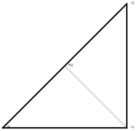
What kind of triangle can be sub-divided into two equal triangles which are each similar to the original one? A moment’s reflection shows that a right angled isosceles triangle has this property. Let us work this out in two dimensions to get a feel for the method before going to the much harder higher dimensional cases. However, it has been shown that for higher dimensions, one can subdivide a $d$ simplex in $n$ dimensions into $n^{d}$ similar simplexes. [7]

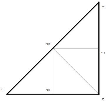
We start with the triangle (Figure 3.1) with vertices $x_{0}=(0,0),\ x_{1}=(a,0),\ x_{2}=(a,a)$. Let

$$F_{a}(\phi_{0},\phi_{1},\phi_{2})=C_{a}e^{-Q_{a}(\phi_{0},\phi_{1},\phi_{2})}$$

be the factor corresponding to such a triangle, for some normalization constant $C_{a}$ and quadratic form $Q_{a}$. We assume that it is invariant under translations in the field variables for simplicity. It is likely that “massless” scalar fields may have this property. If the quadratic term was independent of cross terms between two vertices, it may explain scalar fields in the “infinite mass” limit. Also the interchange of the vertices $1,\>2$ must be a symmetry. Thus we have

$$Q_{a}(\phi_{0},\phi_{1},\phi_{2})=\alpha_{a}\left((\text{$\phi$}_{0}-\phi_{1})^{2}+(\text{$\phi$}_{2}-\text{$\phi$}_{1})^{2}\right)+\beta_{a}(\text{$\phi$}_{0}-\text{$\phi$}_{2})^{2}$$

for some constants $\alpha_{a},\>\beta_{a}.$ This can also be expressed in matrix form as

$$Q_{a}(\phi_{0},\phi_{1},\phi_{2})=\phi^{T}\hat{Q}_{a}\phi,\quad\hat{Q}_{a}=\left(\begin{array}[]{ccc}\alpha_{a}+\beta_{a}&-\alpha_{a}&-\beta_{a}\\ -\alpha_{a}&2\alpha_{a}&-\alpha_{a}\\ -\beta_{a}&-\alpha_{a}&\alpha_{a}+\beta_{a}\end{array}\right)$$

If we choose the new internal vertices to be midpoints of the sides of the original triangle $x_{0}x_{1}x_{2}$

$$x_{ij}=\frac{1}{2}(x_{i}+x_{j}),\quad i,j=0,1,2$$

it divides the original triangle into the four equal triangles that are similar to the original. The new triangles $(x_{0}x_{01}x_{02,}\>x_{02}x_{01}x_{1},\>x_{1}x_{12}x_{02},\>x_{02}x_{12}x_{2})$ have orthogonal edges which are half the length of the original triangle.

Figure 3.1: Refer to caption

The reproducibility condition obtained after integrating out the field variables at the new vertices is

$$e^{-Q_{2a}(\phi_{0},\phi_{1},\phi_{2})}=\int e^{-R_{a}(\phi_{0},\phi_{1},\phi_{2},\phi_{01},\phi_{02},\phi_{12})}d\phi_{01}d\phi_{02}d\phi_{02}$$

where, (up to a normalization constant)

$$R_{a}(\phi_{0},\phi_{1},\phi_{2},\phi_{02})=Q_{a}(\phi_{0},\phi_{01},\phi_{02})+Q_{a}(\phi_{02},\phi_{01},\phi_{1})+Q_{a}(\phi_{1},\phi_{12},\phi_{02})+Q_{a}(\phi_{02},\phi_{12},\phi_{2})$$

This can be expressed in terms of a matrix form as

$$R_{a}(\phi_{0},\phi_{1},\phi_{2},\phi_{01},\phi_{02},\phi_{12})=\phi^{T}\hat{R}_{a}\phi$$

The result of integrating out the new variables $\phi_{01},\phi_{02},\phi_{12}$ is best understood by splitting the matrix $R$ into a block $L$ that acts on the original variables $\left(\phi_{0},\phi_{1},\phi_{2}\right)$ another $K$ acting on the new variables $\left(\phi_{01},\phi_{02},\phi_{12}\right)$ and a third matrix $J$ that mixes the two.

$$\hat{R}_{a}=\left(\begin{array}[]{cc}L&J\\ J^{T}&K\end{array}\right)$$
$$L=\left(\begin{array}[]{ccc}\alpha_{a}+\beta_{a}&0&0\\ 0&2\alpha_{a}+2\beta_{a}&0\\ 0&0&\alpha_{a}+\beta_{a}\end{array}\right)$$
$$K=\left(\begin{array}[]{ccc}4\alpha_{a}&-2\alpha_{a}&0\\ -2\alpha_{a}&4\alpha_{a}+4\beta_{a}&-2\alpha_{a}\\ 0&-2\alpha_{a}&4\alpha_{a}\end{array}\right)$$
$$J=-\left(\begin{array}[]{ccc}\alpha_{a}&\beta_{a}&0\\ \alpha_{a}&2\beta_{a}&\alpha_{a}\\ 0&\beta_{a}&\alpha_{a}\end{array}\right)$$

The exponent in the above Gaussian can also be written as

$$R_{a}(\phi_{0},\phi_{1},\phi_{2},\phi_{01},\phi_{02},\phi_{12})=\phi_{e}^{T}L\phi_{e}+2\phi_{e}^{T}J\phi_{i}+\phi_{i}^{T}K\phi_{i}$$

$\phi_{i}$ and $\phi_{e}$ denote the set of internal (new) and external (original) vertices of the triangle. On completion of squares we get

$$R_{a}=\phi_{e}^{T}L\phi_{e}+(\phi_{i}^{T}+\phi_{e}^{T}J^{T}K^{-1})K(\phi_{i}+K^{-1}J\phi_{e})-\phi_{e}^{T}J^{T}K^{-1}J\phi_{e}$$

The result of the integral over the internal vertices then turns out to be

$$\hat{Q}_{2a}=L_{a}-J_{a}^{T}K_{a}^{-1}J_{a}$$
$$=\left(\begin{array}[]{ccc}\frac{1}{8}(5\alpha_{a}+6\beta_{a})&\frac{1}{2}(-\alpha_{a}-\beta_{a})&\frac{1}{8}(-\alpha_{a}-2\beta_{a})\\ \frac{1}{2}(-\alpha_{a}-\beta_{a})&\alpha_{a}+\beta_{a}&\frac{1}{2}(-\alpha_{a}-\beta_{a})\\ \frac{1}{8}(-\alpha_{a}-2\beta_{a})&\frac{1}{2}(-\alpha_{a}-\beta_{a})&\frac{1}{8}(5\alpha_{a}+6\beta_{a})\end{array}\right)$$

3.1 Fixed Points of the transformation

The above result should be equal to the quadratic form

$$\alpha_{2a}\left[\left(\phi_{0}-\phi_{1}\right)^{2}+\left(\phi_{1}-\phi_{2}\right)^{2}\right]+\beta_{2a}(\phi_{0}-\phi_{2})^{2}=\phi^{T}Q_{2a}\phi$$

On comparing its form we get

$$\alpha_{2a}=\frac{1}{2}(\alpha_{a}+\beta_{a}),\quad\beta_{2a}=\frac{1}{8}(\alpha_{a}+2\beta_{a})$$

If we define the ratio $x_{a}=\frac{\beta_{a}}{\alpha_{a}}$ we can write these relations as

$$x_{2a}=f(x_{a}),\quad f(x)=\frac{1+2x}{4(1+x)}$$
$$\alpha_{2a}=\lambda(x)\alpha_{a},\quad\lambda(x)=\frac{1}{2}(1+x)$$

We now seek a fixed point of the transformation $x_{a}\mapsto x_{2a}$ which is a quadratic equation with two roots

$\displaystyle f(x)$ $\displaystyle=$ $\displaystyle x$
$\displaystyle x$ $\displaystyle=$ $\displaystyle\frac{-1\pm\sqrt{5}}{4}$

The solution with negative $x$ should be discarded as it does not give an integrable Gaussian. The positive root corresponds to the scaling relation

$$\alpha_{2a}=\lambda\alpha_{a},\quad\lambda=\frac{1}{8}\left(3+\sqrt{5}\right)$$

Thus we set

$$x=\frac{\sqrt{5}-1}{4},\quad\lambda=\frac{1}{8}\left(3+\sqrt{5}\right)$$

If we make the ansatz $\alpha_{a}=a^{-\mu}\alpha_{1}$ we get

$$2^{-\mu}=\frac{3+\sqrt{5}}{8}$$

or

$$\mu=\frac{\log(\lambda^{-1})}{\log 2}=\frac{\log\left(\frac{8}{3+\sqrt{5}}\right)}{\log 2}\approx 0.611516$$

In summary, we have a scale covariant solution to the reproducibility condition

$$F_{a}(\phi_{0},\phi_{1},\phi_{2})=C_{a}\exp\left[-a^{-\mu}\alpha_{1}\left\{(\text{$\phi$}_{0}-\phi_{1})^{2}+(\text{$\phi$}_{2}-\text{$\phi$}_{1})^{2}+\frac{\sqrt{5}-1}{4}(\text{$\phi$}_{0}-\text{$\phi$}_{2})^{2}\right\}\right]$$

We can also determine the normalization constant using the relation

$$C_{a}^{4}\sqrt{\frac{\pi^{3}}{32(\alpha_{a}^{3}+2\alpha_{a}^{2}\beta_{a})}}=C_{2a}$$

but that is less interesting.

3.2 Correlation function

Choose two points $x_{1},x_{2}$ on the plane separated by some distance $L=|x_{1}-x_{2}|.$ Draw an iso- right triangle with the line connecting these points as a hypotnuse. We then bisect the right angle to get two iso-right triangles, and subdivide them and so on. After a large number of subdivisions we will get triangles of very small sides. We then integrate out all vertices expect the original triangle to calculate the correlation function:

$$G(x_{1,},x_{2})=\frac{\int\prod_{i}d\phi_{i}\prod_{f}F_{a}\left(\phi(f)\right)\left[\phi(x_{1})-\phi(x_{2})\right]^{2}}{\prod_{i}d\phi_{i}\prod_{f}F_{a}\left(\phi(f)\right)}$$

The integrals can be evaluated using the reproducibility property above. In the end we will end up with an integral over the two vertices of the original large triangle whose side is $L$ :

$$G(x_{1,},x_{2})=\frac{\int d\phi_{0}d\phi_{1}d\phi_{2}\left[\phi_{1}-\phi_{2}\right]^{2}\exp\left[-\frac{L^{-\mu}}{2}\alpha_{1}\left\{\left((\text{$\phi$}_{0}-\phi_{1})^{2}+(\text{$\phi$}_{2}-\text{$\phi$}_{1})^{2}\right)+\frac{\sqrt{5}-1}{4}(\text{$\phi$}_{0}-\text{$\phi$}_{2})^{2})\right\}\right]}{\int d\phi_{1}d\phi_{2}\exp\left[-\frac{L^{-\mu}}{2}\alpha_{1}\left\{\left((\text{$\phi$}_{0}-\phi_{1})^{2}+(\text{$\phi$}_{2}-\text{$\phi$}_{1})^{2}\right)+\frac{\sqrt{5}-1}{4}(\text{$\phi$}_{0}-\text{$\phi$}_{2})^{2})\right\}\right]}\quad$$

Thus, for some positive constant $G$,

$$G(x_{1},x_{2})=G|x_{1}-x_{2}|^{\mu}\sim|x_{1}-x_{2}|^{0.611516}$$

Note that the magnitude of the correlations increase with distance. This is similar to the behavior of the average distance between two points on a Brownian motion. On the other hand this is not the behavior expected from a two dimensional quantum field theory with action $S=-\frac{1}{2}\int|\nabla\phi|^{2}d^{2}x=\frac{1}{2}(\phi,\Delta\phi)$. The correlations behave logarithmically then

$$\int\frac{d^{2}k}{(2\pi)^{2}}\frac{1}{|k|^{2}}e^{ik\cdot(x_{1}-x_{2})}\sim\log|x_{1}-x_{2}|$$

An interpretation is that it is a quantum field theory in a space of fractal dimension in between one and two.

4 Subdividing Tetrahedrons

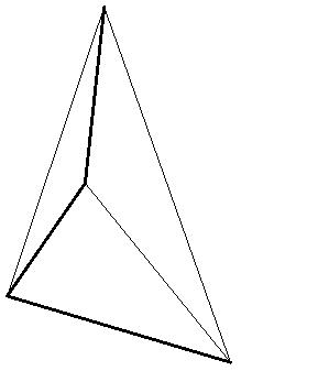
It is not possible to subdivide a tetrahedron into two that are similar to itself by a simple bisection: that would be equivalent to the ancient problem of doubling the cube which is impossible by ruler-compass methods (i.e., the cube root of $2$ cannot be found by such “Platonic” constructions.) But it is possible to subdivide a tetrahedron into eight tetrahedrons, each similar to the original. The trick is to choose right isosceles tetrahedra, whose faces are all right angled triangles, based on three mutually orthogonal edges of equal length[8]. The figure 4.1 shows an example of such a tetrahedron, the three mutually orthogonal edges being shown in bold lines.

Figure 4.1: Refer to caption

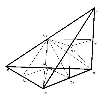
To be more specific, the vertices

$$x_{0}=(0,0,0),\quad x_{1}=(a,0,0),\quad x_{2}=(a,a,0),\quad x_{3}=(a,a,a)$$

gives a right isosceles tetrahedron of smallest side $a$ (Figure 4.2). Every face is a right angled triangle. There are three kinds of edges, of squared lengths $a{}^{2},2a^{2},3a^{2}$. In fact, the squared length of the edge $x_{ij}$ is just $|i-j|a^{2}$, for $i,j=0,1,2,3$. To each such tetrahedron we associate a function $T_{a}(\phi_{0},\phi_{1},\phi_{2},\phi_{3})$ which represents the result of integrating out the field in its interior.

The internal vertices of the subdivision are the six points $x_{ij}=\frac{1}{2}(x_{i}+x_{j})$ for $0\leq i<j\leq 3$.

Figure 4.2: Refer to caption

The reproducibility condition is the integral equation

$\displaystyle T_{2a}(\phi_{0},\phi_{1},\phi_{2},\phi_{3})$ $\displaystyle=$ $\displaystyle\int T_{a}(\phi_{0},\phi_{01},\phi_{02},\phi_{03})T_{a}(\phi_{1},\phi_{01},\phi_{02},\phi_{03})$
$\displaystyle T_{a}(\phi_{1},\phi_{12},\phi_{02},\phi_{03})T_{a}(\phi_{1},\phi_{12},\phi_{13},\phi_{03})T_{a}(\phi_{2},\phi_{12},\phi_{02},\phi_{03})$
$\displaystyle T_{a}(\phi_{2},\phi_{12},\phi_{13},\phi_{03})T_{a}(\phi_{2},\phi_{23},\phi_{13},\phi_{03})T_{a}(\phi_{3},\phi_{23},\phi_{13},\phi_{03})$
$\displaystyle d\phi_{01}d\phi_{02}d\phi_{03}d\phi_{12}d\phi_{13}d\phi_{23}$
Remark 1.

It is important to have the correct order of arguments in the $T_{a}$ as we are not dealing with a regular tetrahedron. We have verified that with the orders given above, (different in detail from the reference above) the distance matrices are exactly half the distance matrix of the original tetrahedron.

We assume a translation symmetry in field space (a global symmetry we expect for massless fields)

$$T_{a}(\phi_{0}+\phi,\phi_{1}+\phi,\phi_{2}+\phi,\phi_{3}+\phi)=T_{a}(\phi_{0},\phi_{1},\phi_{2},\phi_{3})$$

Also, assume a Gaussian ansatz for $T_{a}$.

$\displaystyle T_{a}(\phi_{0},\phi_{1},\phi_{2},\phi_{3})$ $\displaystyle=$ $\displaystyle e^{-Q_{a}(\phi_{0},\phi_{1},\phi_{2},\phi_{3})}$
$\displaystyle Q_{a}(\phi_{0},\phi_{1},\phi_{2},\phi_{3})$ $\displaystyle=$ $\displaystyle\alpha\left((\text{$\phi_{0}$}-\text{$\phi_{1}$})^{2}+(\phi_{3}-\text{$\phi_{2}$})^{2}\right)+\beta\left((\text{$\phi_{0}$}-\text{$\phi_{2}$})^{2}+(\text{$\phi_{3}$}-\text{$\phi_{1}$})^{2}\right)$
$\displaystyle+\gamma(\text{$\phi_{0}$}-\text{$\phi_{3}$})^{2}+\delta(\text{$\phi_{1}$}-\text{$\phi_{2}$})^{2}$

This builds in the translation invariance as well as the reflection symmetry $(0123)\rightleftarrows(3210)$ of the right isosceles tetrahedron.

The exponent of the integral (4) is a quadratic function of ten variables:

$\displaystyle R_{a}(\phi_{0},\phi_{1},\phi_{2},\phi_{3},\phi_{01},\phi_{02},\phi_{03},\phi_{12},\phi_{13},\phi_{23})$ $\displaystyle=$ $\displaystyle Q_{a}(\phi_{0},\phi_{01},\phi_{02},\phi_{03})+Q_{a}(\phi_{1},\phi_{01},\phi_{02},\phi_{03})$
$\displaystyle+Q_{a}(\phi_{1},\phi_{12},\phi_{02},\phi_{03})+Q_{a}(\phi_{1},\phi_{12},\phi_{13},\phi_{03})$
$\displaystyle+Q_{a}(\phi_{2},\phi_{12},\phi_{02},\phi_{03})+Q_{a}(\phi_{2},\phi_{12},\phi_{13},\phi_{03})$
$\displaystyle+Q_{a}(\phi_{2},\phi_{23},\phi_{13},\phi_{03})+Q_{a}(\phi_{3},\phi_{23},\phi_{13},\phi_{03})$

This is equal to $\frac{1}{2}\phi^{T}\hat{R}\phi$ for some $10\times 10$ symmetric matrix $\hat{R}$, which can be calculated by evaluating the second derivatives (Hessian), a straightforward procedure in Mathematica. This matrix can be split into blocks

$$\hat{R}=\left(\begin{array}[]{cc}L&J\\ J^{T}&K\end{array}\right)$$

where $K$ is a matrix in the six dimensional subspace of the internal variables $\left(\phi_{01},\cdots,\phi_{23}\right)$, $L$ is a matrix in the four dimensional subspace of the external variables $\left(\phi_{0},\cdots,\phi_{3}\right)$ and $J$ is a $4\times 6$ matrix that mixes them. The result of evaluating the integral over the internal variables by completing the squares is again a Gaussian with the Hessian matrix

$$L-J^{T}K^{-1}J$$

4.1 Fixed Points of the transformation

Thus we can write the renormalization group transformation as

$$\hat{Q}_{2a}=L_{a}-J_{a}^{T}K_{a}^{-1}J_{a}$$

On comparing with the form of $Q_{a}$, the parameters $\alpha_{2a}\cdots\delta_{2a}$ will be determined as some homogeneous rational functions of $\alpha_{a}\cdots\delta_{a}.$The ratios

$$\frac{\beta_{2a}}{\alpha_{2a}},\frac{\gamma_{2a}}{\alpha_{2a}},\frac{\delta_{2a}}{\alpha_{2a}}$$

depend only on the ratios $x=\frac{\beta_{a}}{\alpha_{a}},y=\frac{\gamma_{a}}{\alpha_{a}},z=\frac{\delta_{a}}{\alpha_{a}}$; i.e. $\alpha_{a}$ and $\alpha_{2a}$ can be scaled out. Thus we get a map of the projective space $P^{3}$ to itself. Each fixed point $(x^{*},y^{*},z^{*})$ of this map is a Gaussian that is mapped into itself under our transformation, except for an overall multiplication of the quadratic form by $\frac{\alpha_{2a}}{\alpha_{a}}$ (the “eigenvalue” $\lambda$) evaluated at $(x^{*},y^{*},z^{*})$. A sensible solution must have a positive eigenvalue and also the parameters $(x^{*},y^{*},z^{*})$ must define a positive quadratic form $Q_{a}$. The equations for the fixed points can be reduced to a polynomial for $x$

$$-2+22x+132x^{2}+380x^{3}+699x^{4}+188x^{5}-1639x^{6}-2488x^{7}-948x^{8}+594x^{9}+608x^{10}+152x^{11}=0$$

The fixed point values for the other variables are determined in terms of this root.

$\displaystyle y$ $\displaystyle=$ $\displaystyle\frac{1}{107606064063}(-88214437948-533552485049x-1626406118465x^{2}-3995440895007x^{3}$
$\displaystyle-4531514030431x^{4}+6599814153205x^{5}+18490138345312x^{6}+10764883382910x^{7}$
$\displaystyle-3123153862430x^{8}-5175977687624x^{9}-1495324502248x^{10})$
$\displaystyle z$ $\displaystyle=$ $\displaystyle\frac{1}{35868688021}(-16477061906-533552485049x-1626406118465x^{2}-3995440895007x^{3}$
$\displaystyle-4531514030431x^{4}+6599814153205x^{5}+18490138345312x^{6}+10764883382910x^{7}$
$\displaystyle-3123153862430x^{8}-5175977687624x^{9}-1495324502248x^{10})$

Of the eleven solutions, only five are real and among them exactly one leads to a positive quadratic form $Q_{a}$

$$x\approx 0.699787174329122,\quad y\approx 0.182495561519144,\quad z\approx 2.547486684557433$$

The eigenvalue i.e. the ratio for this solution is $\frac{\alpha_{2a}}{\alpha_{a}}=\lambda\approx 0.7958942$.

As for the right angled triangles, the correlation function can now be calculated. We can choose any two vertices on the original tetrahedron for this purpose and find the correlation between them. The choice of vertices is not so important as the distance between them is very large compared to the sides of the tetrahedrons obtained by subdivision. The field variables in those vertices obtained by subdivision is integrated out. The correlations will scale as $\lambda^{-1}$ when the distance is doubled. That is,

$$G(x_{1},x_{2})\sim|x_{1}-x_{2}|^{\frac{\log\lambda}{\log 2}}\sim|x_{1}-x_{2}|^{0.329351}$$

5 Additional Examples

5.1 Gaussian Measures

In both cases above we get a correlation function that increases with distance. Are these exponents universal? Is it possible to find another subdivision procedure that will produce a correlation that decreases with distance? To answer these questions we worked out several additional examples of subdivision. It turns out that each subdivision of the plane (into squares, triangles of different shapes etc.) gives a different exponent for the correlation function. Also, in most cases (except two) we get correlation functions that grow with distance.

5.1.1 Subdividing a Square

We can also subdivide the plane into squares (Figure 5.1). To each square of side $a$ we can associate a Gaussian weight with quadratic form

$\displaystyle Q_{a}(\phi_{1},\phi_{2},\phi_{3},\phi_{4})$ $\displaystyle=$ $\displaystyle\alpha_{a}\left[(\phi_{1}-\phi_{2})^{2}+(\phi_{2}-\phi_{3})^{2}+(\phi_{3}-\phi_{4})+(\phi_{4}-\phi_{1})^{2}\right]$
$\displaystyle+\beta_{a}\left[(\phi_{1}-\phi_{3})^{2}+(\phi_{2}-\phi_{4})^{2}\right]$
Figure 5.1: Refer to caption

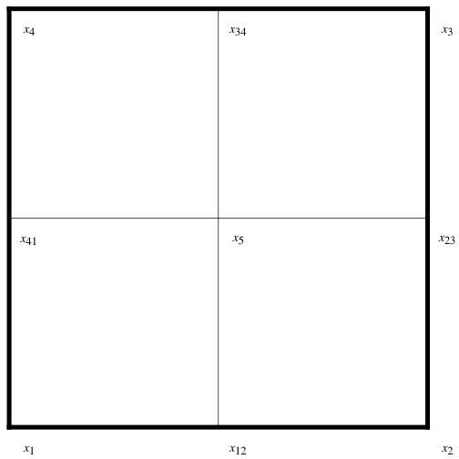
We subdivide each square by connecting the centroid $x_{5}$ to the midpoints of the sides, $x_{12},x_{23},x_{34},x_{41}$. If we then integrate out the five new vertices, we will get the transformations as

$$\alpha_{2a}=\frac{1}{4}(2\alpha_{a}+\beta_{a}),\quad\beta_{2a}=\frac{2\alpha_{a}^{2}+4\alpha_{a}\beta_{a}+\beta_{a}^{2}}{8\alpha_{a}+4\beta_{a}}$$
Fixed Points and Correlation Function

We get the condition for a fixed point of by setting $f(x_{a})=x_{2a}$ where $x_{a}=\frac{\beta_{a}}{\alpha_{a}}$:

$$\frac{4\left(2+4x+x^{2}\right)}{(2+x)(8+4x)}=x$$

Of the three solutions, only $x=-1,\sqrt{3}-1$ lead to positive eigenvalues.

$$\alpha_{2a}=\lambda\alpha_{a},\quad\lambda=\frac{1}{4},\mathrm{or}\ \frac{1}{4}\left(1+\sqrt{3}\right)$$

These two fixed points both give growing correlations

$$G(x_{1}-x_{2})\sim|x_{1}-x_{2}|^{\mu},\quad\mu=2,\mathrm{or}\ 0.550016$$

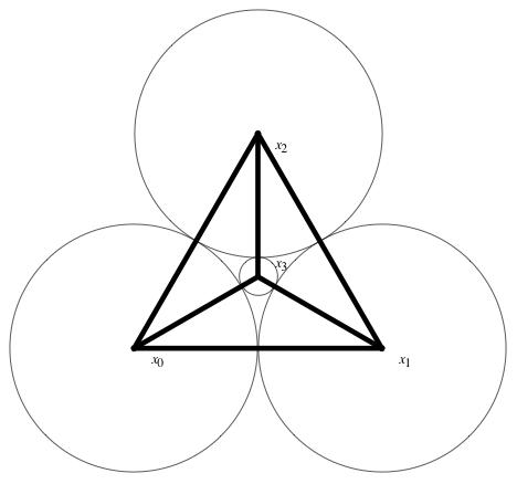
5.1.2 Apollonian Subdivision

Another example of a decreasing correlation function is the iterated Apollonian subdivision of a triangle: we join the vertices to an interior point, thereby subdividing the triangle into three triangles (Figure 5.2). Another interpretation is in terms of circles: we can regard the plane as being subdivided into three mutually tangent circles centered at the vertices of a triangle. Then we can insert a new circle in the interstitial region that is tangent to the other three circle. This process can then be repeated. Every tangency of a pair of circles corresponds to an edge connecting their centers.

Figure 5.2: Refer to caption

The scaling law of the correlation function can be computed just as before by computing the Gaussian integral over the new vertex $x_{3}$

$$e^{-\alpha_{\sqrt{3}a}\left[(\phi_{0}-\phi_{1})^{2}+(\phi_{0}-\phi_{2})^{2}+(\phi_{1}-\phi_{2})^{2}\right]}\propto$$
$$\int e^{-\alpha_{a}\left[(\phi_{0}-\phi_{1})^{2}+(\phi_{0}-\phi_{2})^{2}+(\phi_{1}-\phi_{2})^{2}+2(\phi_{0}-\phi_{3})^{2}+2(\phi_{1}-\phi_{3})^{2}+2(\phi_{2}-\phi_{3})^{2}\right]}d\phi_{3}$$

Each side emanating from vertex $x_{3}$ is shared by two triangles, which explains the factor of two in those terms. The proportionality is given as the scaling is not done rigorously here. We say that one third of the vertices are integrated out roughly after each step and we get $\sqrt{3}$ as the scale factor in two dimensions.

Fixed Points and Correlation Function

This leads to the transformation

$$\alpha_{\sqrt{3}a}=\frac{5}{3}\alpha_{a}$$

and a correlation function with exponent

$$G(x_{1},x_{2})\sim|x_{1}-x_{2}|^{\mu},\quad\mu=\frac{\log\frac{3}{5}}{\log\sqrt{3}}\approx-0.929947$$

Finally we see an example of a correlation decreasing with distance. This may be interpreted as a fractal with dimension greater than two.

5.1.3 Dividing a triangle into six similar triangles

Another example of a decreasing correlation function is the division of an equilateral triangle divided up into six equilateral triangles (Figure 5.3). Topologically this is the same as the barycentric subdivision, or the bisection of the angles of the triangles[9]: we add a new point at the centroid (on the in-center) and connect it to the original vertices and midpoints of the sides. But as long as the six smaller triangles occupy the same plane as the original one, it is not possible for them all to be equilateral. But we can assign equal lengths to all the edges as long as we do not insist that the graph has an isometric embedding in Euclidean space. By iterating the subdivision process, we will get a fractal which makes sense as a metric space, but not as a sub-manifold of Euclidean space.

Figure 5.3: Refer to caption

To each of the equilateral triangle we associate the Gaussian weight

$$Q_{a}(\phi_{0},\phi_{1},\phi_{2})=\alpha_{a}\left[(\phi_{0}-\phi_{1})^{2}+(\phi_{1}-\phi_{2})^{2}+(\phi_{2}-\phi_{0})^{2}\right]$$

The field variables at the vertices $\left(x_{01},x_{02},x_{12}\right)$ and the center of the original triangle $(x_{3})$ are integrated over to give a bigger equilateral triangle with the vertices $\left(x_{0},x_{1},x_{2}\right).$ A side of the newly formed triangle is bigger than the original triangle’s side by a factor of $\sqrt{6}.$

$$e^{-Q_{\sqrt{6}a}(\phi_{0},\phi_{1},\phi_{2})}=\int e^{-R_{a}(\phi_{0},\phi_{1},\phi_{2},\phi_{3},\phi_{01},\phi_{02},\phi_{12})}d\phi_{3}d\phi_{01}d\phi_{12}d\phi_{12}$$

with

$\displaystyle R_{a}(\phi_{0},\phi_{1},\phi_{2},\phi_{3},\phi_{01},\phi_{02},\phi_{12})$ $\displaystyle=$ $\displaystyle Q_{a}(\phi_{0},\phi_{01},\phi_{3})+Q_{a}(\phi_{0},\phi_{3},\phi_{02})+Q_{a}(\phi_{1},\phi_{3},\phi_{01})$
$\displaystyle+Q_{a}(\phi_{1},\phi_{12},\phi_{3})+Q_{a}(\phi_{2},\phi_{3},\phi_{12})+Q_{a}(\phi_{2},\phi_{02},\phi_{3})$
Fixed Points and Correlation Function

On computing the Gaussian integral and comparing it with the Gaussian form expected we get the following transformation

$$\alpha_{\sqrt{6}a}=\frac{5}{4}\alpha_{a}$$

The new quadratic form for the triangle formed will be

$$Q_{\sqrt{6}a}(\phi_{0},\phi_{1},\phi_{2})=\frac{5}{4}\alpha_{a}\left[(\phi_{1}-\phi_{0})^{2}+(\phi_{0}-\phi_{2})^{2}+(\phi_{1}-\phi_{2})^{2}\right]$$

Thus the correlation function scales with exponent as

$$G(x_{1}-x_{2})\sim|x_{1}-x_{2}|^{\mu},\quad\mu=\frac{\log\frac{4}{5}}{\log\sqrt{6}}\approx-0.249078$$

Thus it is possible to get a correlation function that decreases with distance as well.

5.2 Ising Models

5.2.1 The One dimensional Ising Model

We carry out the idea of sub division of the real line once more. However we are now interested in the Ising model now and our field values $(\sigma_{i})$ at the end points of the of the interval can be $\pm 1.$ Instead of integrals we end up doing a discrete sum. Let the function associated with an interval be

$\displaystyle F_{a}(\sigma_{0},\sigma_{1})$ $\displaystyle=$ $\displaystyle e^{Q_{a}(\sigma_{0},\sigma_{1})}$
$\displaystyle Q_{a}(\sigma_{0},\sigma_{1})$ $\displaystyle=$ $\displaystyle\alpha_{a}(\sigma_{0}\sigma_{1})+\gamma_{a}$

There will not be any higher order terms of $\sigma_{i}$ since $\sigma_{i}^{2}=1$ and $\sigma_{i}\sigma_{j}=i\epsilon_{ijk}\sigma_{k}$. We divide the interval into two halves now and the new variable is summed over.

$\displaystyle\sum_{\sigma_{01}}e^{Q_{a}(\sigma_{0},\sigma_{01})}e^{Q_{a}(\sigma_{01},\sigma_{1})}$ $\displaystyle=$ $\displaystyle\sum_{\sigma_{01}}e^{\alpha_{a}\sigma_{01}(\sigma_{0}+\sigma_{1})+2\gamma_{a}}$
$\displaystyle=$ $\displaystyle\left[e^{\alpha_{a}(\sigma_{0}+\sigma_{1})}+e^{-\alpha_{a}(\sigma_{0}+\sigma_{1})}\right]e^{2\gamma_{a}}$
Fixed Points and Correlation Function

On comparing with the function associated with the whole interval

$$F_{2a}(\sigma_{0},\sigma_{1})=e^{\alpha_{2a}(\sigma_{0}\sigma_{1})+\gamma_{2a}}$$

we get the following pair of equations considering all the combinations formed by the pair $\left(\sigma_{0},\sigma_{1}\right)$

$\displaystyle 2e^{2\gamma_{a}}$ $\displaystyle=$ $\displaystyle e^{\gamma_{2a}-\alpha_{2a}}$
$\displaystyle e^{2\gamma_{a}}\left(e^{2\alpha_{a}}+e^{-2\alpha_{a}}\right)$ $\displaystyle=$ $\displaystyle e^{\gamma_{2a}+\alpha_{2a}}$

The transformation obtained from these equations is

$$e^{2\alpha_{2a}}=\frac{e^{2\alpha_{a}}+e^{-2\alpha_{a}}}{2}$$

The trivial fixed point $\alpha_{a}=0$ is obtained by setting $\alpha_{2a}=\alpha_{a}.$ The normalization constant can be determined from the relation between $\gamma_{a}$ and $\gamma_{2a}$.

5.2.2 Ising Model on the Fractal Subdivision of a Right Angled Triangle

We carry out the idea of sub division for a triangle now (Figure 5.4). Let the function associated with the triangle be

$\displaystyle F_{a}(\sigma_{0},\sigma_{1},\sigma_{2})$ $\displaystyle=$ $\displaystyle e^{Q_{a}(\sigma_{0},\sigma_{1},\sigma_{2})}$
$\displaystyle Q_{a}(\sigma_{0},\sigma_{1},\sigma_{2})$ $\displaystyle=$ $\displaystyle\alpha_{a}(\sigma_{0}\sigma_{1}+\sigma_{1}\sigma_{2})+\beta_{a}(\sigma_{0}\sigma_{2})+\gamma_{a}$
Figure 5.4: Refer to caption

We now divide the original triangle in two new similar triangles. The new vertex is summed over and the total contribution from the two triangles is computed.

$\displaystyle\sum_{\sigma_{02}}e^{Q_{a}(\sigma_{1},\sigma_{02},\sigma_{0})}e^{Q_{a}(\sigma_{2},\sigma_{02},\sigma_{1})}$ $\displaystyle=$ $\displaystyle\sum_{\sigma_{02}}e^{\alpha_{a}\sigma_{02}(\sigma_{0}+\sigma_{2}+2\sigma_{1})+\beta_{a}\sigma_{1}(\sigma_{0}+\sigma_{2})+2\gamma_{a}}$
$\displaystyle=$ $\displaystyle\left[e^{\alpha_{a}(\sigma_{0}+\sigma_{2}+2\sigma_{1})}+e^{-\alpha_{a}(\sigma_{0}+\sigma_{2}+2\sigma_{1})}\right]e^{\beta_{a}\sigma_{1}(\sigma_{0}+\sigma_{2})+2\gamma_{a}}$
Fixed Points and Correlation Function

On comparing it with the form of the energy associated with the bigger triangle

$$F_{\sqrt{2}a}(\sigma_{0},\sigma_{1},\sigma_{2})=e^{\alpha_{\sqrt{2}a}\sigma_{1}(\sigma_{0}+\sigma_{2})+\beta_{\sqrt{2}a}(\sigma_{0}\sigma_{2})+\gamma_{\sqrt{2}a}}$$

we get the following pairs of equations

$\displaystyle e^{2(\gamma_{a}+\beta_{a})}\left(e^{4\alpha_{a}}+e^{-4\alpha_{a}}\right)$ $\displaystyle=$ $\displaystyle e^{2\alpha_{\sqrt{2}a}+\beta_{\sqrt{2}a}+\gamma_{\sqrt{2}a}}$
$\displaystyle e^{2\gamma_{a}}\left(e^{2\alpha_{a}}+e^{-2\alpha_{a}}\right)$ $\displaystyle=$ $\displaystyle e^{-\beta_{\sqrt{2}a}+\gamma_{\sqrt{2}a}}$
$\displaystyle 2e^{2(\gamma_{a}-\beta_{a})}$ $\displaystyle=$ $\displaystyle e^{-2\alpha_{\sqrt{2}a}+\beta_{\sqrt{2}a}+\gamma_{\sqrt{2}a}}$

In order to obtain these equations we look into all the tuples formed by assigning values to $\left(\sigma_{0},\sigma_{1},\sigma_{2}\right).$ Out of the set of eight equations we get only three independent equations. The transformations obtained from these equations are

$\displaystyle e^{4\alpha_{\sqrt{2}a}}$ $\displaystyle=$ $\displaystyle\frac{e^{4\beta_{a}}\left(e^{4\alpha_{a}}+e^{-4\alpha_{a}}\right)}{2}$
$\displaystyle e^{4\beta_{\sqrt{2}\alpha}}$ $\displaystyle=$ $\displaystyle\frac{2\left(e^{4\alpha_{a}}+e^{-4\alpha_{a}}\right)}{\left(e^{2\alpha_{a}}+e^{-2\alpha_{a}}\right)^{2}}$

The trivial fixed points $\alpha_{a}=0,\>\beta_{a}=0$ are obtained by setting $\alpha_{\sqrt{2}a}=\alpha_{a},\>\beta_{\sqrt{2}a}=\beta_{a}$. $\gamma_{a}$ and $\gamma_{\sqrt{2}a}$ determine the normalization factor.

5.2.3 Ising Model on sixfold subdivision of the triangle

After having found trivial fixed points $\alpha_{a}=0$ till now we take up the example of the sixfold subdivision of the triangle to see if it has a non trivial fixed point. And indeed it has one. To each of the equilateral triangles we associate a function as shown below.

$\displaystyle F_{a}(\sigma_{0},\sigma_{1},\sigma_{2})$ $\displaystyle=$ $\displaystyle e^{Q_{a}(\sigma_{0},\sigma_{1},\sigma_{2})}$
$\displaystyle Q_{a}(\sigma_{0},\sigma_{1},\sigma_{2})$ $\displaystyle=$ $\displaystyle\alpha_{a}(\sigma_{0}\sigma_{1}+\sigma_{1}\sigma_{2}+\sigma_{2}\sigma_{0})+\gamma_{a}$

A sum is now carried over the vertices $(\sigma_{01},\sigma_{02},\sigma_{12},\sigma_{3})$ to form a bigger equilateral triangle with the vertices $(\sigma_{0},\sigma_{1},\sigma_{2})$.

$\displaystyle\sum_{\sigma_{01}}\sum_{\sigma_{02}}\sum_{\sigma_{12}}\sum_{\sigma_{3}}e^{Q_{a}(\sigma_{1},\sigma_{12},\sigma_{3})}e^{Q_{a}(\sigma_{2},\sigma_{12},\sigma_{3})}e^{Q_{a}(\sigma_{2},\sigma_{02},\sigma_{3})}e^{Q_{a}(\sigma_{0},\sigma_{02},\sigma_{3})}e^{Q_{a}(\sigma_{0},\sigma_{01},\sigma_{3})}e^{Q_{a}(\sigma_{1},\sigma_{01},\sigma_{3})}$
$\displaystyle=$ $\displaystyle e^{-6\alpha_{a}+6\gamma_{a}}(2+e^{-2(-2+\sigma_{2}+\sigma_{0})\alpha_{a}}+e^{2(2+\sigma_{2}+\sigma_{0})\alpha_{a}}+e^{-2(-2+\sigma_{2}+\sigma_{1})\alpha_{a}}+e^{2(2+\sigma_{2}+\sigma_{1})\alpha_{a}}$
$\displaystyle+e^{-2(-2+\sigma_{0}+\sigma_{1})\alpha_{a}}+e^{2(2+\sigma_{0}+\sigma_{1})\alpha_{a}}+e^{-4(-3+\sigma_{2}+\sigma_{0}+\sigma_{1})\alpha_{a}}+e^{4(3+\sigma_{2}+\sigma_{0}+\sigma_{1})\alpha_{a}}$
$\displaystyle+e^{-2(-4+2\sigma_{2}+\sigma_{0}+\sigma_{1})\alpha_{a}}+e^{2(4+2\sigma_{2}+\sigma_{0}+\sigma_{1})\alpha_{a}}+e^{-2(-4+\sigma_{2}+2\sigma_{0}+\sigma_{1})\alpha_{a}}+e^{2(4+\sigma_{2}+2\sigma_{0}+\sigma_{1})\alpha_{a}}$
$\displaystyle+e^{-2(-4+\sigma_{2}+\sigma_{0}+2\sigma_{1})\alpha_{a}}+e^{2(4+\sigma_{2}+\sigma_{0}+2\sigma_{1})\alpha_{a}})$
Fixed Points and Correlation Function

The function associated with the bigger triangle should be of the form

$$F_{\sqrt{6}a}(\sigma_{0},\sigma_{1},\sigma_{2})=e^{\alpha_{\sqrt{6}a}(\sigma_{1}\sigma_{0}+\sigma_{0}\sigma_{2}+\sigma_{2}\sigma_{1})+\gamma_{\sqrt{6}a}}$$

We get the following pairs of equations on comparing the two results.

$\displaystyle e^{-\alpha_{\sqrt{6}a}+\gamma_{\sqrt{6}a}}$ $\displaystyle=$ $\displaystyle e^{-6(\alpha_{a}-\gamma_{a})}\left(3+6e^{4\alpha_{a}}+4e^{8\alpha_{a}}+2e^{12\alpha_{a}}+e^{16\alpha_{a}}\right)$
$\displaystyle e^{3\alpha_{\sqrt{6}a}+\gamma_{\sqrt{6}a}}$ $\displaystyle=$ $\displaystyle e^{-6(\alpha_{a}-\gamma_{a})}\left(9+3e^{8\alpha_{a}}+3e^{16\alpha_{a}}+e^{24\alpha_{a}}\right)$

Thus the renormalization group transformation on $\alpha$ is the iteration of the function

$$f(\alpha)=\frac{-1}{4}\text{log}\left[\frac{3+6e^{4\alpha_{a}}+4e^{8\alpha_{a}}+2e^{12\alpha_{a}}+e^{16\alpha_{a}}}{9+3e^{8\alpha_{a}}+3e^{16\alpha_{a}}+e^{24\alpha_{a}}}\right]$$

There is a trivial fixed point for the equation $\alpha_{a}=f(\alpha_{a})$ at $\alpha_{a}=0$ and a non trivial fixed point at $\alpha_{a*}=0.159579$. The normalization constants are determined by $\gamma_{a}$ and $\gamma_{\sqrt{6}a}.$

To find the critical exponents we linearize the recursion relation at the fixed point[5].

$$f^{\prime}(\alpha_{a*})=1.93411$$

This shows that the fixed point is unstable. The scaling factor for this transformation is $\sqrt{6}.$ Using these numbers we can calculate the thermal exponent $y_{t}\simeq\frac{\log(1.93411)}{\log(\sqrt{6})}=0.736312$. This leads to the critical exponents for the correlation length and specific heat to be $\nu=\frac{1}{y_{t}}=1.35812,\>\alpha=2(1-\nu)=-0.716239$.

6 Acknowledgement

It is a pleasure to thank Sreedhar B. Dutta, Tamar Friedman, Govind Krishnaswami, Yannick Meurice, Fred Moolekamp, Ambar Sengupta and S. Shankaranarayanan for discussions. This work was supported in part by a grant from the US Department of Energy under contract DE-FG02-91ER40685.

References

  • [1] K. Ito, Lectures on Stochastic Processes, Notes by M.Rao, TIFR (1961)
  • [2] H. A. Bethe, Proc. Roy. Soc. London Ser A, 150 ( 1935 ), pp. 552-575
  • [3] For a review, see Y. Meurice, J. Phys. A: Math. Theor. 40 (2007) R39–R102
  • [4] R. Strichartz , Analysis on Fractals, Notices Amer. Math. Soc. 46 (1999), 1199–1208
  • [5] M. Kardar, Statistical Physics of Fields,Cambridge University Press (2007).
  • [6] G. Calcagni, JHEP03(2010)120[arXiv:1004.5144v2]; K. Svozil, J. Phys. A: Math. Gen. 20 (1987) 3861-3875
  • [7] H. Edelsbrunner,and D. R. Grayson, Discrete & Computational Geometry Volume 24, Number 4, 707-719
  • [8] A. Plazaa, M.A. Padr?nb, J.P. Su?rezc, S. Falc?na Finite Elements in Analysis and Design 41 (2004) 253–265
  • [9] S. Butler and Graham arXiv:1007.2301v1