Nature of the antiferromagnetic quantum phase transition on the honeycomb lattice

Abstract

We address the nature of the antiferromagnetic quantum phase transition that separates a semimetal from an antiferromagnet in the repulsive Hubbard model defined on the honeycomb lattice. At the critical point, the fermions acquire an anomalous dimension $\eta$ due to their strong coupling to the fluctuations of the order parameter $\phi$. The finite $\eta$ in turn induces a singular $\phi^{4}$ term and a non-analytical spin susceptibility signaling the breakdown of Hertz’s $\phi^{4}$ theory. As a result, the continuous antiferromagnetic quantum phase transition is internally unstable and turns into a first order transition.

Quantum phase transitions are believed to be present in a wide variety of correlated quantum matter ranging from strongly correlated electron systems to ultracold quantum gases on engineered lattices understand . Such quantum phase transitions occur at zero temperature as a function of a non-thermal tuning parameter Sachdevbook ; understand ; Vojta ; Sachdev . Understanding the nature of possible quantum phase transitions of a given system and describing the ensuing physical behaviors present a great challenge of modern materials science. In particular, the possible zero-temperature phase transitions in various models of interacting electrons on the two-dimensional honeycomb lattice have recently generated intense theoretical and numerical interests Herbut06 ; Herbut09 ; Honerkamp ; Sorella ; Hermele ; Wangfa ; Ran ; Wen ; Meng ; Sachdev ; Fritz . While it is well-established that the ground state of the repulsive Hubbard model is a semimetal (SM) at weak coupling and a Mott-insulating antiferromagnet (AFM) at strong coupling, the nature of the transition between these two phases is still not well understood.

There are generally two scenarios for the transition from a SM to an AFM. Herbut Herbut06 ; Herbut09 studied the repulsive Hubbard model on a honeycomb lattice by means of a renormalization group (RG) method in the large-$N$ limit and argued that the strong on-site interaction drives a direct, continuous SM-AFM quantum phase transition, which is in qualitative agreement with the results obtained by a functional RG calculation Honerkamp and early quantum Monte Carlo (MC) simulations Sorella . Treatments of the Hubbard models based on auxiliary-particle methods on the contrary seem to indicate that various exotic quantum spin liquid phases may exist between the SM and AFM phases Hermele ; Wangfa ; Ran ; Wen . Particularly, a recent quantum MC simulation Meng found an intermediate gapped spin liquid phase. These two scenarios are apparently contradictory, and no consensus has been reached so far.

The theoretical study of quantum phase transitions was pioneered by Hertz Hertz , who developed a field-theoretic approach to describe the (anti-)ferromagnetic phase transition in an itinerant electron system. In this approach, the fermionic degrees of freedom are completely integrated out, yielding an effective $\phi^{4}$ action soley in terms of an order parameter $\phi$. Hertz’s theory and its generalizations Millis ; Moriya have been applied to numerous quantum phase transitions Sachdevbook ; Vojta . Recently, however, the general validity of this approach has been called into question Vojta ; Belitz ; Abanov ; Chubukov as it has become clear that it is not always eligible to integrate out all fermionic degrees of freedom in an itinerant electron system. Indeed, the singular interaction between gapless itinerant fermions and order parameter fluctuations can lead to important features that are beyond a simple $\phi^{4}$ description Vojta ; Belitz ; Abanov ; Chubukov .

In this Letter we address the nature of the quantum phase transition between an antiferromagnet and a semimetal on the honeycomb lattice. We approach the problem by assuming that the SM-AFM phase transition is a continuous one and then examining whether it is stable or not. To this end, we maintain the fermionic degrees of freedom of the system, described as massless Dirac fermions, within a Yukawa-type field theory to describe the SM-AFM quantum critical point. This allows for a careful study of the singular interaction between Dirac fermions and order parameter fluctuations.

We first compute the fermion anomalous dimension after incorporating the damping effects of both Dirac fermions and order parameter. We then calculate the coefficient of an effective quartic $\phi^{4}$ term and the spin susceptibility, and show that both of these two quantities are non-analytical. As it turns out, the non-analytical spin susceptibility leads to an effective energy of $\phi$ that has a minimum at a finite momentum $q_{c}$, so a nonzero AFM order parameter is generated at the transition point. This order parameter is nonuniform and spatially modulated as $\langle\phi\rangle=\phi_{0}e^{\mathbf{q}_{c}\cdot\mathbf{x}}$. All these unusual behaviors indicate that, the original Hertz $\phi^{4}$ theory breaks down and the Dirac fermions and order parameter fluctuations should be treated equally. As we demonstrate below, the putative continuous SM-AFM quantum phase transition is destroyed by the critical order parameter fluctuations and consequently becomes first order.

We begin with the half-filled Hubbard model

$$\mathcal{H}=-\sum_{<i,j>}tc_{i\sigma}^{\dagger}c_{j\sigma}+\sum_{i}U\left(n_{i\uparrow}-\frac{1}{2}\right)\left(n_{i\uparrow}-\frac{1}{2}\right)$$ (1)

defined on a two-dimensional honeycomb lattice. Here, $n_{i\alpha}=c_{i\sigma}^{\dagger}c_{i\sigma}$ and $c_{i\sigma}^{\dagger}$ ($c_{i,\sigma}$) creates (destroys) an electron of spin projection $\sigma$ at site $i$. The sum $<i,j>$ is over nearest neighbors and the hoping $t$ is taken to be a constant. A band structure analysis shows that the conduction band touches the valence band at discrete points, so the low-energy excitations are massless Dirac fermions. Around the touching Dirac points, the kinetic term can be converted to a free Lagrangian term

$$\mathcal{L}_{0}=\sum_{\sigma}\bar{\Psi}_{\sigma}(\partial_{\tau}\gamma_{0}-iv_{F}\partial_{x}\gamma_{1}-iv_{F}\partial_{y}\gamma_{2})\Psi_{\sigma},$$ (2)

where $\gamma_{0}=\mathbbm{1}\otimes\tau_{3}$, $\gamma_{1}=\mathbbm{1}\otimes i\tau_{1}$, and $\gamma_{2}=\tau_{3}\otimes i\tau_{2}$. The $4$-component spinor $\Psi_{\sigma}$ represents Dirac fermion, and is arranged as $\Psi_{\sigma}=(c_{AK\sigma},c_{BK\sigma},c_{AK^{\prime}\sigma},c_{BK^{\prime}\sigma})^{T}$ with sublattice indices $A,B$ and valley indices $K,K^{\prime}$. Its conjugate is $\bar{\Psi}_{\sigma}=\Psi^{\dagger}_{\sigma}\gamma_{0}$. The on-site Hubbard interaction can be rewritten as the sum of a number of continuum four-fermion interaction terms, among which only the following term turns out to be relevant in the RG sense Herbut06 ,

$$\mathcal{L}_{\mathrm{int}}=-\frac{2g}{N}\Big{(}\sum_{\sigma}\sigma\bar{\Psi}_{\sigma}(\tau,\mathbf{r})\Psi_{\sigma}(\tau,\mathbf{r})\Big{)}^{2},$$ (3)

where $g=Ua^{2}/8$ and $a$ is the lattice constant.

We first sketch Hertz’s approach Hertz . It is convenient to introduce a scalar field $\phi$ and perform a Hubbard-Stratonovich transformation, yielding

$$\mathcal{L}=\mathcal{L}_{0}+\frac{N}{2}\left[(\partial_{\tau}\phi)^{2}+(\mathbf{\nabla}\phi)^{2}+r\phi^{2}\right]-\phi\sum_{\sigma}\sigma\bar{\Psi}_{\sigma}\Psi_{\sigma}.$$ (4)

Integrating out the fermion fields $\bar{\Psi},\Psi$ and taking the saddle point approximation leads to a gap equation Rosenstein

$$\frac{\langle\phi\rangle}{g}=16\int_{\omega,\mathbf{k}}\frac{\langle\phi\rangle}{\omega^{2}+{\mathbf{k}}^{2}+\langle\phi\rangle^{2}}.$$ (5)

The critical point separating zero and finite expectation value $\langle\phi\rangle$ is given by $\frac{1}{g_{c}}=16\int_{\omega,\mathbf{k}}\frac{1}{\omega^{2}+\mathbf{k}^{2}}$. For $g<g_{c}$, the system is in the gapless SM phase with $\langle\phi\rangle=0$. For $g>g_{c}$, $\langle\phi\rangle\neq 0$, so the Dirac fermions acquire a finite mass gap and the system is turned to a Mott insulator. Such excitonic-type insulating transition is a condensed-matter analog of the dynamical fermion-mass generation mechanism proposed originally in particle physics Nambu . The order parameter can be expressed in terms of fermion operators as $\langle\phi\rangle=\langle\sum_{\sigma}\sigma\bar{\Psi}_{\sigma}\Psi_{\sigma}\rangle$, so the Mott insulator is indeed an AFM. Close to $g_{c}$, the fermion gap is approximated by $\langle\phi\rangle=\frac{\pi}{4}\left(\frac{1}{g_{c}}-\frac{1}{g}\right)$, which suggests that the SM-AFM transition is continuous. This phase transition is tuned by the parameter $r=\frac{1}{4}\left(\frac{1}{g}-\frac{1}{g_{c}}\right)$, with $g_{c}$ defining the zero-temperature quantum critical point.

Figure 1: (a) the dressed boson propagator; (b) the one-loop diagram for the polarization function; (c) the fermion self-energy diagram.

We will now demonstrate that Hertz’ scenario of the SM-AFM transition on the honeycomb lattice can be fundamentally altered by the coupling between Dirac fermions and critical order parameter fluctuations. This coupling describes the decay of composite order parameter into single fermionic excitations as well as the formation of order parameter by fermion pairing. Since it affects the dynamics of both fermions and bosons, we are led to maintain the fermions in the Yukawa-type theory, Eq. (4), and study the fermions and bosons on equal footings. This will be done by analyzing the Yukawa interaction by means of an $1/N$ expansion where $N$ represents the fermion flavor (spin).

Due to the Lorentz invariance of the action in the low-energy sector, the dynamical exponent is $z=1$. The free fermion propagator is $G_{0}(\omega,\mathbf{k})=\frac{1}{i\omega\gamma_{0}-\mathbf{\gamma\cdot k}}$. In leading order of $1/N$ expansion, the polarization is given by

$$\Pi_{0}(\Omega,\mathbf{q})=\int_{\omega,\mathbf{k}}\mathrm{Tr}\left[G_{0}(\omega,\mathbf{k})G_{0}(\omega+\Omega,\mathbf{k+q})\right],$$ (6)

and shown in Fig. 1(b). It follows that $\Pi_{0}(\Omega,\mathbf{q})=\frac{1}{4}\sqrt{\Omega^{2}+\mathbf{q}^{2}}$. The bosonic propagator at the same order in $1/N$ is therefore $D^{-1}(\Omega,\mathbf{q})=N\left[\Omega^{2}+q^{2}+\Pi_{0}(\Omega,\mathbf{q})\right]$. In the low energy regime, the free terms turn out to be unimportant, so $D(\Omega,\mathbf{q})=\frac{4}{N\sqrt{\Omega^{2}+\mathbf{q}^{2}}}$. The leading fermion self-energy diagram is shown in Fig. 1(c). Retaining the most divergent part leads to $\Sigma_{0}(\omega,\mathbf{k})=-\frac{2}{3\pi^{2}N}(i\omega\gamma_{0}-\mathbf{\gamma\cdot k})\ln\left(\frac{\Lambda}{\sqrt{\omega^{2}+\mathbf{k}^{2}}}\right)$. From the Dyson equation, $G^{-1}(\omega,\mathbf{k})=i\omega\gamma_{0}-\mathbf{\gamma\cdot k}-\Sigma_{0}(\omega,\mathbf{k})$, this results in a dressed fermion propagator

$$G(\omega,\mathbf{k})=-\frac{i\omega\gamma_{0}-\mathbf{\gamma\cdot k}}{(\omega^{2}+\mathbf{k}^{2})^{1-\frac{\eta}{2}}},$$ (7)

with anomalous dimension $\eta=\frac{2}{3\pi^{2}N}$. This propagator implies the absence of a well-defined quasiparticle pole.

So far, our calculation is on the level of random phase approximation since the polarization $\Pi_{0}(\Omega,\mathbf{q})$ has been obtained from the free propagator $G_{0}(\omega,\mathbf{k})$. However, $\Pi_{0}(\Omega,\mathbf{q})$ may be considerably modified when the feedback of fermion dressing is included. Replacing $G_{0}(\omega,\mathbf{k})$ by $G(\omega,\mathbf{k})$ shown in Eq.(7), we obtain a new polarization

$$\Pi_{0}^{\prime}(\Omega,\mathbf{q})=A(\eta)(\Omega^{2}+\mathbf{q}^{2})^{\frac{1}{2}+\eta},$$ (8)

where $A(\eta)$ is a well-defined function of $\eta$ . The fermion self-energy and anomalous dimension $\eta$ may also be altered, so it is necessary to recalculate the fermion self-energy by including the dressing effects of both fermions and bosons. Using the dressed expressions, Eqs. (7) and (8), we get a new fermion self-energy $\Sigma(\omega,\mathbf{k})=-\frac{B(\eta)}{8\pi^{3}NA(\eta)}\frac{i\omega\gamma_{0}-\mathbf{\gamma\cdot k}}{(\omega^{2}+\mathbf{k}^{2})^{\frac{\eta}{2}}}$, where $B(\eta)$ is another function of $\eta$ . Replacing $\Sigma_{0}(\omega,\mathbf{k})$ by $\Sigma(\omega,\mathbf{k})$, we are again lead to Eq.(7). The dressed fermion propagator $G(\omega,\mathbf{k})$ thus survives the self-consistency analysis.

We are now in a position to examine the validity of Hertz’s $\phi^{4}$ theory and the stability of the continuous SM-AFM quantum phase transition. According to Hertz Hertz , one can formally integrate out all fermionic degrees of freedom and obtain an effective action as a function of the order parameter $\phi$:

$$S_{\mathrm{eff}}[\phi]=\int_{\Omega,\mathbf{q}}\left[\chi_{2}(\Omega,\mathbf{q})\phi^{2}+\chi_{4}(\Omega,\mathbf{q})\phi^{4}+O(\phi^{6})\right].$$ (9)

Here, the quadratic coefficient is determined by the spin susceptibility: $\chi_{2}(\Omega,\mathbf{q})=\Omega^{2}+\mathbf{q}^{2}+\Pi(\Omega,\mathbf{q})$. The validity of this $\phi^{4}$ theory is rooted on the basic assumption that the coefficients $\chi_{2}(\Omega,\mathbf{q})$ and $\chi_{4}(\Omega,\mathbf{q})$ are regular in $\Omega,\mathbf{q}$.

We first consider the coefficient of the quartic $\phi^{4}$ term. According to the leading diagram shown in Fig. 2, it is

$$\chi_{4}(\Omega,\mathbf{q}) = \int\frac{d\omega d^{2}\mathbf{k}}{(2\pi)^{3}}\mathrm{Tr}\left[G(\omega,\mathbf{k})G(\omega+\Omega,\mathbf{k+q})\right.$$ (10)

$$\left.\times G(\omega,\mathbf{k})G(\omega+\Omega,\mathbf{k+q})\right].$$

Using the dressed fermion propagator Eq.(7) and carrying out some tedious calculations, one can show that

$$\chi_{4}(\Omega,\mathbf{q})=\frac{F(\eta)}{(\Omega^{2}+\mathbf{q}^{2})^{\frac{1}{2}-2\eta}},$$ (11)

with

$$F(\eta) \propto \frac{2\Gamma(4-2\eta)}{\Gamma^{2}(2-\eta)}\left[\frac{3}{2}\frac{\Gamma(\frac{1}{2}-2\eta)}{\Gamma(3-2\eta)}+\frac{\Gamma(\frac{5}{2}-2\eta)}{\Gamma(4-2\eta)}\right.$$

$$\left.-\frac{13}{2}\frac{\Gamma(\frac{3}{2}-2\eta)}{\Gamma(4-2\eta)}\right]\int_{0}^{1}\frac{dx}{[x(1-x)]^{-\frac{1}{2}-\eta}}$$

$$+\left[\frac{\Gamma(\frac{3}{2}-2\eta)}{\Gamma^{2}(2-\eta)}-\frac{\Gamma(\frac{1}{2}-2\eta)}{\Gamma^{2}(1-\eta)}\right]\int_{0}^{1}\frac{dx}{[x(1-x)]^{\frac{1}{2}-\eta}}.$$

The function $F(\eta)$ is finite for any finite $\eta$ and it is easy to see that $\chi_{4}(\Omega,\mathbf{q})$ is divergent in the $\Omega,\mathbf{q}\rightarrow 0$ limit. In other words, the quartic $\phi^{4}$ term is singular. An important feature of $F(\eta)$ is that it vanishes in the absence of fermion anomalous dimension, i.e., $F(\eta=0)=0$, thus, this singularity is absent if the free propagator $G_{0}(\omega,\mathbf{k})$ is used. Therefore, the singularity in $\chi_{4}(\Omega,\mathbf{q})$ arises directly from the critical order parameter fluctuations, which is reflected in the finiteness of $\eta$.

Figure 2: $\phi^{4}$ vertex correction at the one-loop level.

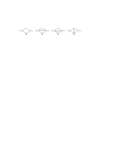
Figure 3: Polarization functions up to the two-loop level.

We now turn to analyze the spin susceptibility at the quantum critical point. For the effective $\phi^{4}$ theory to be applicable and the continuous SM-AFM transition to be stable, the static spin susceptibility $\chi_{2}(\mathbf{q})$ should have a regular momentum dependence. It is commonly believed that the spin susceptibility of a Fermi liquid is regular. Interestingly, Belitz et al. demonstrated that a nonanalytic spin susceptibility in a clean Fermi liquid system can occur Belitz . Subsequently, Chubukov et al. obtained a negative, nonanalytic spin susceptibility for a ferromagnetic quantum phase transition system with dynamical exponent $z=3$ Chubukov . It is therefore necessary to check whether the spin susceptibility is regular or singular.

The spin susceptibility actually corresponds to the polarization function $\Pi(q)$. The leading diagram is shown as Fig. 3(a), with $\Pi_{2}^{a}(\Omega,\mathbf{q})$ being already given by Eq.(8). The two-loop contributions are represented by the three diagrams (b), (c), and (d) of Fig. 3. Using Eqs. (7) and (8), we find that the sum of (b) and (c) is

$$\Pi_{2}^{b+c}(\Omega,\mathbf{q})=-2C_{1}(\eta)\Pi_{2}^{a}(\Omega,\mathbf{q}),$$ (12)

where $C_{1}(\eta)=\frac{B(\eta)}{8\pi^{3}NA(\eta)}$. Employing a method used in Franz and then performing a lengthy computation, we find

$$\Pi_{2}^{d}(\Omega,\mathbf{q})=-2C_{2}(\eta)\ln\Big{(}\frac{\Lambda}{\sqrt{\Omega^{2}+\mathbf{q}^{2}}}\Big{)}\Pi_{2}^{a}(\Omega,\mathbf{q}),$$ (13)

where $C_{2}(\eta)$ is a function of $\eta$. Adding $\Pi_{2}^{a}$, $\Pi_{2}^{b+c}$, and $\Pi_{2}^{d}$ together one arrives at the expression

$$\Pi_{2}(\Omega,\mathbf{q}) = \left(\Omega^{2}+\mathbf{q}^{2}\right)^{-\frac{\eta^{\prime}}{2}}\Pi_{2}^{a}(\Omega,\mathbf{q})-2C_{1}(\eta)\Pi_{2}^{a}(\Omega,\mathbf{q})$$

$$\propto \Big{[}\left(\Omega^{2}+\mathbf{q}^{2}\right)^{-\frac{\eta^{\prime}}{2}}-2C_{1}(\eta)\Big{]}\left(\Omega^{2}+\mathbf{q}^{2}\right)^{\frac{1}{2}+\eta},$$

where $\eta^{\prime}=-2C_{2}(\eta)$. Since $\eta^{\prime}<0$, the function $\Pi_{2}(\Omega,\mathbf{q})$ is positive for large $\Omega,\mathbf{q}$ but becomes negative for $\Omega,\mathbf{q}$ below a given threshold. As a result, the corresponding spin susceptibility $\chi_{2}(\Omega,\mathbf{q})$ is non-analytical.

As with the $\chi_{4}$ term, this non-analyticity is directly related to the fermion anomalous dimension: If we assume $\eta=0$ and apply the free fermion propagator $G_{0}(\omega,\mathbf{k})$, then $\Pi_{2}^{a}(\Omega,\mathbf{q})$ is identical to $\Pi^{0}(\Omega,\mathbf{q})$ given by Eq.(6), and both $\Pi_{2}^{b+c}(\Omega,\mathbf{q})$ and $\Pi_{2}^{d}(\Omega,\mathbf{q})$ are proportional to $\ln\Big{(}\frac{\Lambda}{\sqrt{\Omega^{2}+\mathbf{q}^{2}}}\Big{)}\Pi^{0}(\Omega,\mathbf{q})$. The total polarization for $\eta=0$ will be $\Pi_{2}(\Omega,\mathbf{q},\eta=0)\propto(\Omega^{2}+\mathbf{q}^{2})^{\frac{1}{2}+\frac{8}{3\pi^{2}N}}$, which is positive and analytical.

Based on the above analysis, we arrive at a key conclusion: the non-analyticities in $\chi_{4}(\Omega,\mathbf{q})$ and $\chi_{2}(\Omega,\mathbf{q})$ clearly signal the breakdown of Hertz’s $\phi^{4}$ theory. Moreover, the non-analytical spin susceptibility will alter the nature of the SM-AFM transition. To demonstrate this, we write the effective action for $\phi$ as $S_{\mathrm{eff}}[\phi]=\int_{q}\left[\left(q^{2}+\Pi_{2}(q)\right)\phi^{2}+\chi_{4}(q)\phi^{4}\right]$ with $\Pi_{2}(q)$ given by Eq.(14). To determine its ground state, one needs to find the minimum of the total energy. The absolute minimum of kinetic energy $E_{q}=q^{2}+\Pi_{2}(q)$ is located at a finite momentum $q_{c}$, which is one of the solutions of equation $dE_{q}/dq=0$. Though it is hard to derive an analytical expression of $q_{c}$, its finiteness can be easily confirmed by numerical computation. Inserting $q_{c}$ to $E_{q}$, we find that the non-analytical spin susceptibility leads to a negative minimal kinetic energy, i.e., $E_{q_{c}}^{\mathrm{min}}<0$. Around $q_{c}$, $E_{q}$ can be approximated by $E_{q}\approx E_{q_{c}}^{\mathrm{min}}+\kappa(q-q_{c})^{2}$ with certain constant $\kappa$. Originally, at the critical point $g=g_{c}$, the scalar field $\phi$ has a vanishing mass, $r=0$, so the potential energy is simply $V[\phi]\propto\phi^{4}$ and one should expect $\langle\phi\rangle=0$. However, the finite $E_{q_{c}}^{\mathrm{min}}$ induced by non-analytical spin susceptibility serves as an effective, negative mass. Moreover, $\chi_{4}(q)$ is regular for finite $q_{c}$, and hence can be safely replaced by a constant. Consequently, the effective potential becomes $V[\phi]=-\left|E_{q_{c}}^{\mathrm{min}}\right|\phi^{2}+\chi_{4}(q_{c})\phi^{4}$, which yields a finite expectation value, $\langle\phi\rangle=\left[-E_{q_{c}}^{\mathrm{min}}/2\chi_{4}(q_{c})\right]^{\frac{1}{2}}$, even if $r=0$. According to the generic analysis of Brazovskii Brazovskii , this nonzero order parameter $\langle\phi\rangle$ should be nonuniform. By minimizing the corresponding free energy, we find the order parameter is spatially modulated as $\phi(\mathbf{x})=\phi_{0}e^{i\mathbf{q}_{c}\cdot\mathbf{x}}$.

In the SM phase with $r>0$, the order parameter fluctuation is gapped, so the Yukawa interaction does not generate any fermion anomalous dimension. As explained in the above discussions, $\chi_{2}(\omega,\mathbf{q})$ and $\chi_{4}(\omega,\mathbf{q})$ exhibit no singular behaviors when $\eta=0$, thus the spin susceptibility is analytical for $r>0$ and non-analytical only at the critical point $r=0$. Therefore, $\langle\phi\rangle$ vanishes for any positive $r$, but develops a finite magnitude at $r=0$ discontinuously because of the negativeness of $E_{q_{c}}^{\mathrm{min}}$. Apparently, although SM-AFM phase transition is shown to be continuous by the gap equation analysis, it is ultimately driven first order due to singular interaction between order parameter and massless Dirac fermions.

In summary, we analyzed the nature of the quantum phase transition between a semimetal and an antiferromagnet on a honeycomb lattice. We demonstrated that the strong interaction between massless Dirac fermions and critical order parameter fluctuations generates unexpected properties. As a consequence, the original Hertz $\phi^{4}$ theory is incomplete for this problem and the massless fermions should be treated on equal footing with the critically fluctuating order parameter. This behavior arises from the non-vanishing fermion anomalous dimension, which in turn reflects strong damping effects that need to be included. Our results indicate that, although the SM-AFM transition is continuous at the mean-field level, it is destroyed by the critical order parameter fluctuations and actually gives way to a first order transition with a spatially modulated order parameter. The anticipated quantum critical phenomena of continuous SM-AFM transition Sachdev ; Herbut06 ; Herbut09 ; Fritz are not expected to exist.

G.Z.L. acknowledges support by the National Natural Science Foundation of China under grant No.11074234 and the Visitors Program of MPIPKS at Dresden.

References

- (1) Understanding Quantum Phase Transitions, edited by L. D. Carr (CRC Press, 2011).
- (2) S. Sachdev, Quantum Phase Transitions (Cambridge University Press, 2000).
- (3) Ar. Abanov et al., Adv. Phys. 52, 119 (2003); M. Vojta, Rep. Prog. Phys. 66, 2069 (2003); D. Belitz et al., Rev. Mod. Phys. 77, 579 (2005); H. v. Lhneysen et al., Rev. Mod. Phys. 79, 1015 (2008); P. Gegenwart et al., Nat. Phys. 4, 186 (2008).
- (4) S. Sachdev, arXiv:1012.0299v3.
- (5) I. F. Herbut, Phys. Rev. Lett. 97, 146401 (2006).
- (6) I. F. Herbut et al., Phys. Rev. B 79, 085116 (2009); Phys. Rev. B 80, 075432 (2009).
- (7) L. Fritz, Phys. Rev. B 83, 035125 (2011).
- (8) C. Honerkamp, Phys. Rev. Lett. 100, 146404 (2008).
- (9) S. Sorella and E. Tosatti, Europhys. Lett. 19, 699 (1992); T. Pavia et al., Phys. Rev. B 72, 085123 (2005).
- (10) M. Hermele, Phys. Rev. B 76, 035125 (2007).
- (11) F. Wang, Phys. Rev. B 82, 024419 (2010).
- (12) Y. M. Lu and Y. Ran, Phys. Rev. B 84, 024420 (2011).
- (13) A. Vaezi and X.-G. Wen, arXiv:1010.5744.
- (14) Z. Y. Meng et al., Nature (London) 464, 847 (2010).
- (15) J. Hertz, Phys. Rev. B 14, 1165 (1976).
- (16) A. J. Millis, Phys. Rev. B 48, 7183 (1993).
- (17) T. Moriya, Spin Fluctuations in Itinerant Electron Magnetism (Springer-Verlag, Berlin, New York, 1995).
- (18) D. Belitz et al., Phys. Rev. B 55, 9452 (1997).
- (19) A. V. Chubukov et al., Phys. Rev. Lett. 92, 147003 (2004); J. Rech et al., Phys. Rev. B 74, 195126 (2006).
- (20) A. Abanov and A. V. Chubukov, Phys. Rev. Lett. 93, 255702 (2004).
- (21) B. Rosenstein et al., Phys. Rep. 205, 59 (1991).
- (22) Y. Nambu and G. Jona-Lasinio, Phys. Rev. 122, 345 (1961).
- (23) M. Franz et al., Phys. Rev. B 68, 024518 (2003).
- (24) S. A. Brazovskii, Sov. Phys. JETP 41, 85 (1975).