Preference-based Search using Example-Critiquing with Suggestions

Abstract

We consider interactive tools that help users search for their most preferred item in a large collection of options. In particular, we examine example-critiquing, a technique for enabling users to incrementally construct preference models by critiquing example options that are presented to them. We present novel techniques for improving the example-critiquing technology by adding suggestions to its displayed options. Such suggestions are calculated based on an analysis of users’ current preference model and their potential hidden preferences. We evaluate the performance of our model-based suggestion techniques with both synthetic and real users. Results show that such suggestions are highly attractive to users and can stimulate them to express more preferences to improve the chance of identifying their most preferred item by up to $78\%$.

1 Introduction

The internet makes an unprecedented variety of opportunities available to people. Whether looking for a place to go for vacation, an apartment to rent, or a PC to buy, the potential customer is faced with countless possibilities. Most people have difficulty finding exactly what they are looking for, and the current tools available for searching for desired items are widely considered inadequate. Artificial intelligence provides powerful techniques that can help people address this essential problem. Search engines can be very effective in locating items if users provide the correct queries. However, most users do not know how to map their preferences to a query that will find the item that most closely matches their requirements.

Recommender systems (?, ?, ?) address this problem by mapping explicit or implicit user preferences to items that are likely to fit these preferences. They range from systems that require very little input from the users to more user-involved systems. Many collaborative filtering techniques  (?), infer user preferences from their past actions, such as previously purchased or rated items. On the other hand, popular comparison websites often require that users state at least some preferences on desired attribute values before producing a list of recommended digital cameras, portable computers, etc.

In this article, we consider tools that provide recommendations based on explicitly stated preferences, a task that we call preference-based search. In particular, the problem is defined as:

Given a collection ${\cal O}=\{o_{1},..,o_{n}\}$ of $n$ options, preference-based search (PBS) is an interactive process that helps users identify the most preferred option, called the target option $o_{t}$, based on a set of preferences that they have stated on the attributes of the target.

Tools for preference-based search face a tradeoff between two conflicting design goals:

• decision accuracy, measured as the percentage of time that the user finds the target option when using the tool, and

• user effort, measured as the number of interaction cycles or task time that the user takes to find the option that she believes to be the target using the tool.

By target option, we refer to the option that a user prefers most among the available options. To determine the accuracy of a product search tool, we measure whether the target option a user finds with the tool corresponds to the option that she finds after reviewing all available options in an offline setting. This procedure, also known as the switching task, is used in consumer decision making literature (?). Notice that such procedure is only used to measure the accuracy of a system. We do not suggest that such procedure models human decision behavior.

In one approach, researchers focus purely on accuracy in order to help users find the most preferred choice. For example, Keeney and Raiffa (?) suggested a method to obtain a precise model of the user’s preferences. This method, known as the value function assessment procedure, asks the user to respond to a long list of questions. Consider the case of search for an ideal apartment. Suppose the decision outcome involves trading off some preferred values of the size of an apartment against the distance between the apartment and the city center. A typical assessment question is in the form of “All else being equal, which is better: 30 sqm at 60 minutes distance or 20 sqm at 5 minutes distance?” Even though the results obtained in this way provide a precise model to determine the most preferred outcome for the user, this process is often cognitively arduous. It requires the decision maker to have a full knowledge of the value function in order to articulate answers to the value function assessment questions. Without training and expertise, even professionals are known to produce incomplete, erroneous, and inconsistent answers (?). Therefore, such techniques are most useful for well-informed decision makers, but less so for users who need the help of a recommender system.

Recently, researches have made significant improvement to this method. ? (?) consider a prior probability distribution of a user’s utility function and only ask questions having the highest value of information on attributes that will give the highest expected utility. Even though it was developed for decision problems under uncertainty, this adaptive elicitation principle can be used for preference elicitation for product search which is often modeled as decision with multiple objectives (see in the related work section the approach of ?). ? (?) and ? (?) further improved this method by taking into account the value assigned to future preference elicitation questions in order to further reduce user effort by modeling the maximum possible regret as a stopping criterion.

In another extreme, researchers have emphasized providing recommendations with as little effort as possible from the users. Collaborative filtering techniques (?), for example, infer an implicit model of a user’s preferences from items that they have rated. An example of such a technique is Amazon’s “people who bought this item also bought…” recommendation. However, users may still have to make a significant effort in assigning ratings in order to obtain accurate recommendations, especially as a new user to such systems (known as the new user problem). Other techniques produce recommendations based on a user’s demographic data (?, ?).

1.1 Mixed Initiative Based Product Search and Recommender Systems

In between these two extremes, mixed-initiative dialogue systems have emerged as promising solutions because they can flexibly scale user’s effort in specifying their preferences according to the benefits they perceive in revealing and refining preferences already stated. They have been also referred to as utility and knowledge-based recommender systems according to Burke (?), and utility-based decision support interface systems (DSIS) according to Spiekermann and Paraschiv (?). In a mixed-initiative system, the user takes the initiative to state preferences, typically in reaction to example options displayed by the tool. Thus, the user can provide explicit preferences as in decision-theoretic methods, but is free to flexibly choose what information to provide, as in recommender systems.

The success of these systems depends not only on the AI techniques in supporting the search and recommending task, but also on an effective user-system interaction model that motivates users to state complete and accurate preferences. It must strike the right compromise between the recommendation accuracy it offers and the effort it requires from the users. A key criterion to evaluate these systems is therefore the accuracy vs. effort framework which favors systems that offer maximum accuracy while requiring the same or less user effort. This framework was first proposed by ? (?) while studying user behaviors in high-stake decision making settings and later adapted to online user behaviors in medium-stake decision making environments by Pu and Chen (?) and Zhang and Pu (?).

In current practice, a mixed-initiative product search and recommender system computes its display set (i.e., the items presented to the user) based on the closeness of these items to a user’s preference model. However, this set of items is not likely to provide for diversity and hence may compromise on the decision accuracy. Consider for example a user who is looking for a portable PC and gives a low price and a long battery life as initial preferences. The best matching products are all likely to be standard models with a 14-inch display and a weight around 3 kilograms. The user may thus never get the impression that a good variety is available in weight and size, and may never express any preferences on these criteria. Including a lighter product in the display set may greatly help a user identify her true choice and hence increase her decision accuracy.

Recently, the need for recommending not only the best matches, called the candidates, but also a diverse set of other items, called suggestions, has been recognized. One of the first to recognize the importance of suggestive examples was ATA (?), which explicitly generated examples that showed the extreme values of certain attributes, called extreme examples. In case-based recommender systems, the strategy of generating both similar and diverse cases was used (?, ?). ? (?) investigated algorithms for generating similar and diverse solutions in constraint programming, which can be used to recommend configurable products. The complexity of such algorithms was further analyzed.

So far, the suggestive examples only aim at providing a diverse set of items without analyzing more deeply whether variety actually helps users make better decisions. One exception is the compromise-driven diversity generation strategy by McSherry (?) who proposes to suggest items which are representative of all possible compromises the user might be prepared to consider. As Pu and Li (?) pointed out, tradeoff reasoning (making compromises) can increase decision accuracy, which indicates that the compromise-driven diversity might have a high potential to achieve better decision quality for users. However, no empirical studies have been carried out to prove this.

1.2 Contribution of Our Work

We consider a mixed-initiative framework with an explicit preference model, consisting of an iterative process of showing examples, eliciting critiques and refining the preference model. Users are never forced to answer questions about preferences they do not yet possess. On the other hand, their preferences are volunteered and constructed, not directly asked. This is the key difference between navigation-by-proposing used in the mixed-initiative user interaction model as opposed to value assessment-by-asking used in traditional decision support systems.

With a set of simulated and real-user involved experiments, we argue that including diverse suggestions among the examples shown by a mixed initiative based product recommender is a significant improvement in the state-of-the-art in this field. More specifically, we show that the model-based suggestion techniques that we have developed indeed motivate users to express more preferences and help them achieve a much higher level of decision accuracy without additional effort.

The rest of this article is organized as follows. We first describe a set of model-based techniques for generating suggestions in preference-based search. The novelty of our method includes: 1) it expands a user’s current preference model, 2) it generates a set of suggestions based on an analysis of the likelihood of the missing attributes, and 3) it displays suggested options whose attractiveness stimulates users’ preference expression. To validate our theory, we then examine how suggestion techniques help users identify their target choice in both simulation environments and with real users. We base the evaluation of these experiments on two main criteria. Firstly, we consider the completeness of a user’s preference model as measured by preference enumeration, i.e., the number of features for which a user has stated preferences. The higher the enumeration, the more likely a user has considered all aspects of a decision goal, and therefore the decision is more likely to be rational. Secondly, we consider decision accuracy as measured by the contrary of the switching rate, which is the number of users who did not find their target option using the tool and choose another product after reviewing all options in detail. The smaller the switching rate, the more likely a user is content with what she has chosen using the tool, and thus the higher decision accuracy.

The success of the suggestion techniques is confirmed by experimental evaluations. An online evaluation was performed with real users exploring a student housing database. A supervised user study was additionally carried out with 40 users, performed in a within-subject experiment setup that evaluated the quantitative benefits of model-based suggestion. The results demonstrate that model-based suggestion increased decision accuracy by up to $78\%$, while the user’s effort is about the same as using the example-critiquing search tool without suggestions. Such user studies which consider the particular criteria of accuracy vs. effort have never been carried out by other researchers for validating suggestion strategies or optimal elicitation procedures.

Finally, we end by reviewing related works followed by a conclusion.

2 Example-critiquing

In many cases, users searching for products or information are not very familiar with the available items and their characteristics. Thus, their preferences are not well established, but constructed while learning about the possibilities (?). To allow such construction to take place, a search tool should ask questions with a complete and realistic context, not in an abstract way.

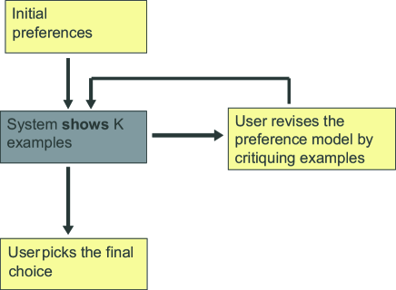
Figure 1: Example-critiquing interaction. The dark box is the computer’s action, the other boxes show actions of the user.

A good way to follow this principle is to implement an example critiquing interaction (see Figure 1). It shows examples of available options and invites users to state their critique of these examples. This allows users to better understand their preferences.

Example-critiquing has been proposed by numerous researchers in two main forms: systems without and with explicit preference models:

• in systems without preference models, the user proceeds by tweaking the current best example (“I like this but cheaper”,“I like this but French cuisine”) to make it fit with his or her preferences better. The preference model is represented implicitly by the currently chosen example and the interaction is that of navigation-by-proposing. Examples of such systems are the FindMe systems (?, ?), the ExpertClerk system (?), and the dynamic critiquing systems (?).

• in systems with preference models, each critique is added to an explicit preference model that is used to refine the query. Examples of systems with explicit preference models include the ATA system (?), SmartClient (?), and more recently incremental critiquing (?).

In this article, we focus on example-critiquing with an explicit preference model for the advantage of effectively resolving users’ preference conflicts. Moreover, this approach not only helps users make a particular choice, but also obtains an accurate preference model for future purchases or cross-domain recommendations.

2.1 Example

As a simple example consider a student looking for housing. Options are characterized by the following 4 attributes:

1. rent in Swiss Francs;

2. type of accommodation: room in a shared apartment, studio, or apartment

3. distance to the university in minutes;

4. furnished/unfurnished.

Assume that the choice is among the following options:

	rent	type-of-accommodation	distance-to-university	furnished
$o_{1}$	400	room	17	yes
$o_{2}$	500	room	32	yes
$o_{3}$	600	apartment	14	no
$o_{4}$	600	studio	5	no
$o_{5}$	650	apartment	32	no
$o_{6}$	700	studio	2	yes
$o_{7}$	800	apartment	7	no

Assume that the user initially only articulates a preference for the lowest price. She also has hidden preferences for an unfurnished accomodation, and a distance of less than 10 minutes to the university. None of the options can satisfy all of these preferences, so the most suitable option requires the user to make a tradeoff among her preferences. Let us assume that the tradeoffs are such that option $o_{4}$ would be the user’s most preferred option. We call this the target option.

The user may start the search with only the first preference (lowest price), and the tool would show the $k$ best options according to the order shown in the table. Here, let $k=1$ so that only option $o_{1}$ is shown.

In an example-critiquing tool without a preference model, the user indicates a critique of the currently shown example, and the system then searches for another example that is as similar as possible to the current one while also satisfying the critique. In this case, the user might critique $o_{1}$ for being furnished, and the tool might then show $o_{3}$ which is most similar to the unfurnished preference. The user might add the critique that the option should be at most 10 minutes from the university, and the system would then return $o_{7}$ as the most similar option that satisfies this critique. The user might again critique this option as being too expensive, in which case the system would return to $o_{3}$ as most similar to the preference on the ”cheaper” option. As there is no memory of earlier critiques, the process is stuck in a cycle, and the user can never discover the target $o_{4}$.

In a tool with a preference model, the user is able to state her preference for an unfurnished option, making $o_{3}$ the best option. Next, she might add the additional preference for a distance of less than 10 minutes to the university, ending up with $o_{4}$ which is her target choice. This illustrates how an explicit preference model ensures the convergence of the process. In fact, decision theory shows that when all preferences have been expressed, a user will always be able to identify the target choice. Note however that more complex scenarios might require explicit tradeoffs among preferences to locate the right target choice (?).

A popular approach to obtain a preference model is to elicit it by asking questions to the user. However, this can lead to means objectives (?) that distract from the true target choice. As an example, the tool might first ask the user whether she prefers a room, a studio or an apartment. If the user truly has no preference, she might try to translate her preference for an unfurnished option into a preference for an apartment, since this is most likely to be unfurnished. However, this is not her true preference and will shift the best tradeoff from $o_{4}$ to $o_{3}$ or even $o_{7}$. This illustrates the importance of a mixed-initiative approach where the user can state preferences in any order on her own initiative.

The example-critiquing framework raises issues of how to model preferences, how to generate the solutions shown to the user, and how to efficiently implement the process. We now briefly summarize the results of our previous work addressing these issues.

2.2 Preference Modeling

When a tool forces users to formulate preferences using particular attributes or a particular order, they can fall prey to means objectives (?) because they do not have the catalog knowledge to relate this to their true intentions. Means objectives are objectives that a person believes to correlate positively to the true objectives. For example, a manufacturer with a reputation for good quality may become an objective when it is impossible to state an objective on the quality itself.

To avoid such means objectives, we require a preference model that allows users to state preferences incrementally using any attribute, in any order they wish. Furthermore, the preference model must be easy to revise at each critiquing cycle by adding or removing preferences.

This rules out commonly used techniques such as question-answer dialogues or selection of a fixed set of preferences that are commonly used on the web today.

An effective formalism that satisfies these criteria is to formulate preferences using soft constraints. A soft constraint is a function from an attribute or a combination of attributes to a number that indicates the degree to which the constraint is violated. More generally, the values of a soft constraint can be elements of a semiring (?). When there are several soft constraints, they are combined into a single preference measure. Examples of combination operators are summing or taking the maximum. The overall preference order of outcomes is then given by this combined measure.

For example, for an attribute that can take values a, b and c, a soft constraint indicating a preference for value b could map a and c to 1, and b to 0, thus indicating that only b does not violate the preference. A preference for the surface area to be at least 30 square meters, where a small violation of up to 5 square meters could be acceptable, can be expressed by a piecewise linear function:

$$1 \mbox{if }x<25$$

$$0.2(30-x) \mbox{if }25\leq x\leq 30$$

$$0 \mbox{if }x>30$$

In example-critiquing, each critique can be expressed as a soft constraint, and the preference model is incrementally constructed by simply collecting the critiques. Note that it is also possible for a user to express several preferences involving the same attributes, for example to express in one soft constraint that the surface area should be at least 30 square meters (as above), and in another soft constraint that it should be no more than 50 square meters. If the soft constraints are combined by summing their effects, this result leads to a piecewise linear function:

$$1 \mbox{if }x<25$$

$$0.2(30-x) \mbox{if }25\leq x\leq 30$$

$$0 \mbox{if }30<x<50$$

$$0.2(x-50) \mbox{if }50\leq x\leq 55$$

$$1 \mbox{if }x>55$$

Thus, soft constraints allow users to express relatively complex preferences in an intuitive manner. This makes soft constraints a useful model for example-critiquing preference models. Furthermore, there exist numerous algorithms that combine branch-and-bound with constraint consistency techniques to efficiently find the most preferred options in the combined order. More details on how to use soft constraints for preference models are provided by Pu & Faltings (?).

However soft constraints are a technique that allows a user to partially and incrementally specify her preferences. The advantage over utility functions is that it is not necessary to elicit a user’s preference for every attribute. Only attributes whose values concern the current decision context are elicited. For example, if a user is not interested in a certain brand of notebooks, then she does not have to concern herself with stating preferences on those products. This parsimonious approach is similar to the adaptive elicitation method proposed by Chajewska et al. (?). However, in example-critiquing for preference-based search, user’s preferences are volunteered as reactions to the displayed examples, not elicited; users are never forced to answer questions about preferences without the benefit of a concrete decision context.

2.3 Generating Candidate Choices

In general, users are not able to state each of their preferences with numerical precision. Instead, a practical tool needs to use an approximate preference model where users can specify their preferences in a qualitative way.

A good way to implement such a preference model is to use standardized soft constraints where numerical parameters are chosen to fit most users. Such models will necessarily be inaccurate for certain users. However, this inaccuracy can be compensated by showing not just one, but a set of $k$ best candidate solutions. The user then chooses the most preferred one from this set, thus compensating for the preference model’s inaccuracy. This technique is commonly used in most search engines.

We have analyzed this technique for several types of preference models: weighted soft constraints, fuzzy-lexicographic soft constraints, and simple dominance relations (?).

A remarkable result is that for both weighted and fuzzy-lexicographic constraint models, assuming a bound on the possible error (deviation between true value and the one used by the application) of the soft constraints modeling the preferences, the probability that the true most preferred solution is within $k$ depends only on the number of the preferences and the error bound of the soft constraints but not on the overall size of the solution set. Thus, it is particularly suitable when searching a very large space of items.

We also found that if the preference model contains many different soft constraints, the probability of finding the most preferred option among the $k$ best quickly decreases. Thus, compensating model inaccuracy by showing many solutions is only useful when preference models are relatively simple. Fortunately, this is often the case in preference-based search, where people usually lack the patience to input complex models.

As a result, the most desirable process in practice might be a two-stage process where example-critiquing with a preference model is used in the first stage to narrow down the set of options from a large (thousands) space of possibilities to a small (20) most promising subset. The second phase would use a tweaking interaction where no preference model is maintained to find the best choice. Pu and Chen (?) have shown tradeoff strategies in a tweaking interaction that provide excellent decision accuracy even when user preferences are very complex.

2.4 Practical Implementation

Another challenge for implementing example-critiquing in large scale practical settings is that it requires solutions to be computed specifically for the preference model of a particular user. This may be a challenge for web sites with many users.

However, it has been shown (?, ?) that the computation and data necessary for computing solutions can be coded in very compact form and run as an applet on the user’s computer. This allows a completely scaleable architecture where the load for the central servers is no higher than for a conventional web site. Torrens, Faltings & Pu (?) describe an implementation of example-critiquing using this architecture in a tool for planning travel arrangements. It has been commercialized as part of a tool for business travelers (?).

3 Suggestions

In the basic example-critiquing cycle, we can expect users to state any additional preference as long as they perceive it to bring a better solution. The process ends when users can no longer see potential improvements by stating additional preferences and have thus reached an optimum. However, since the process is one of hill-climbing, this optimum may only be a local optimum. Consider again the example of a user looking for a notebook computer with a low price range. Since all of the presented products have about the same weight, say around 3 kg, she might never bother to look for lighter products. In marketing science literature, this is called the anchoring effect (?). Buyers are likely to make comparisons of products against a reference product, in this case the set of displayed heavy products. Therefore, a buyer might not consider the possibility of a lighter notebook that might fit her requirements better, and accept a sub-optimal result.

Just as in hillclimbing, such local minima can be avoided by randomizing the search process. Consequently, several authors have proposed including additional examples selected in order to educate the user about other opportunities present in the choice of options (?, ?, ?, ?). Thus, the displayed examples would include:

• candidate examples that are optimal for the current preference query, and

• suggested examples that are chosen to stimulate the expression of preferences.

Different strategies for suggestions have been proposed in literature. Linden (?) used extreme examples, where some attribute takes an extreme value. Others use diverse examples as suggestions (?, ?, ?).

Consider again the example of searching for housing mentioned in the previous section. Recall that the choice is among the following options:

	rent	type-of-accommodation	distance-to-university	furnished
$o_{1}$	400	room	17	yes
$o_{2}$	500	room	32	yes
$o_{3}$	600	apartment	14	no
$o_{4}$	600	studio	5	no
$o_{5}$	650	apartment	32	no
$o_{6}$	700	studio	2	yes
$o_{7}$	800	apartment	7	no

In the initial dialogue with the system, the user has stated the preference of lowest price. Consequently, the options are ordered $o_{1}\succ o_{2}\succ o_{3}=o_{4}\succ o_{5}\succ o_{6}\succ o_{7}$.

Assume that the system shows only one candidate, which is the most promising option according to the known preferences: $o_{1}$. What other options should be shown as suggestions to motivate the user to express her remaining preferences?

Linden et al. (?) proposed using extreme examples, defined as examples where some attribute takes an extreme value. For example, consider the distance: $o_{6}$ is the example with the smallest distance. However, it has a much higher price, and being furnished does not satisfy the user’s other hidden preference. Thus, it does not give the user the impression that a closer distance is achievable without compromising her other preferences. Only when the user wants a distance of less than 5 minutes can option $o_{6}$ be a good suggestion, otherwise $o_{4}$ is likely to be better. Another problem with extreme examples is that we need two such examples for each attribute, which is usually more than the user can absorb.

Another strategy (?, ?, ?, ?, ?) is to select suggestions to achieve a certain diversity, while also observing a certain goodness according to currently known preferences. As the tool already shows $o_{1}$ as the optimal example, the most different example is $o_{5}$, which differs in all attributes but does not have an excessive price. So is $o_{5}$ a good suggestion? It shows the user the following opportunities:

• apartment instead of room: however, $o_{3}$ would be a cheaper way to achieve this.

• distance of 32 instead of 17 minutes: however, $o_{2}$ would be a cheaper way to achieve this.

• unfurnished instead of furnished: however, $o_{3}$ would be a cheaper way to achieve this.

Thus, while $o_{5}$ is very diverse, it does not give the user an accurate picture of what the true opportunities are. The problem is that diversity does not consider the already known preferences, in this case price, and the dominance relations they imply on the available options. While this can be mitigated somewhat by combining diversity with similarity measures, for example by using a linear combination of both (?, ?), this does not solve the problem as the effects of diversity should be limited to attributes without known preferences while similarity should only be applied to attributes with known preferences.

We now consider strategies for generating suggestions based on the current preference model. We call such strategies model-based suggestion strategies.

We assume that the user is minimizing his or her own effort and will add preferences to the model only when he or she expects them to have an impact on the solutions. This is the case when:

• the user can see several options that differ in a possible preference, and

• these options are relevant, i.e. they could be acceptable choices, and

• they are not already optimal for the already stated preferences.

In all other cases, stating an additional preference is irrelevant: when all options would evaluate the same way, or when the preference only has an effect on options that would not be eligible anyway or that are already the best choices, stating it would be wasted effort. On the contrary, upon display of a suggested outcome whose optimality becomes clear only if a particular preference is stated, the user can recognize the importance of stating that preference. This seems to be confirmed by our user studies.

This has led us to the following principle, which we call the look-ahead principle, as a basis for model-based suggestion strategies:

Suggestions should not be optimal under the current preference model, but should provide a high likelihood of optimality when an additional preference is added.

We stress that this is a heuristic principle based on assumptions about human behavior that we cannot formally prove. However, it is justified by the fact that suggestion strategies based on the look-ahead principle work very well in real user studies, as we report later in this article.

In the example, $o_{4}$ and $o_{3}$ have the highest probability of satisfying the lookahead principle: both are currently dominated by $o_{1}$. $o_{4}$ becomes Pareto-optimal when the user wants a studio, an unfurnished option, or a distance of less than 14 minutes. $o_{3}$ becomes Pareto-optimal when the user wants an apartment, an unfurnished option, or a distance of less than 17 minutes. Thus, they give a good illustration of what is possible within the set of examples.

We now develop our method for computing suggestions and show that how it can generate these suggestions.

3.1 Assumptions about the Preference Model

To further show how to implement model-based suggestion strategies, we have to define preference models and some minimal assumptions about the shape that user preferences might take. We stress that these assumptions are only made for generating suggestions. The preference model used in the search tool could be more diverse or more specific as required by the application.

We consider a collection of options ${\cal O}=\{o_{1},..,o_{n}\}$ and a fixed set of $k$ attributes $A=\{A_{1},..,A_{k}\}$, associated with domains $D_{1},..,D_{n}$. Each option $o$ is characterized by the values $a_{1}(o),...,a_{k}(o)$; where $a_{i}(o)$ represents the value that $o$ takes for attribute $A_{i}$.

A qualitative domain (the color, the name of neighborhood) consists in an enumerated set of possibilities; a numeric domain has numerical values (as price, distance to center), either discrete or continuous. For numeric domains, we consider a function $range(Att)$ that gives the range on which the attribute domain is defined. For simplicity we call qualitative (respectively numeric) attributes those with qualitative (numeric) domains.

The user’s preferences are assumed to be independent and defined on individual attributes:

Definition 1

A preference $r$ is an order relation $\preceq_{r}$ of the values of an attribute $a$; $\sim_{r}$ expresses that two values are equally preferred. A preference model R is a set of preferences $\{r_{1},..,r_{m}\}$.

Note that $\preceq_{r}$ might be a partial or total order.

If there can be preferences over a combination of attributes, such as the total travel time in a journey, we assume that the model includes additional attributes that model these combinations so that we can make the assumption of independent preferences on each attribute. The drawback is that the designer has to know the preferential dependence in advance. However, this is required for designing the user interface anyway.

As a preference $r_{i}$ always applies to the same attribute $a_{i}$, we simplify the notation and apply $\preceq_{r_{i}}$ and $\sim_{r_{i}}$ to the options directly: $o_{1}\prec_{r_{i}}o_{2}$ iff $a_{i}(o_{1})\prec_{r_{i}}a_{i}(o_{2})$. We use $\prec_{r_{i}}$ to indicate that $\preceq_{r_{i}}$ holds but not $\sim_{r_{i}}$.

Depending on the formalism used for modeling preferences, there are different ways of combining the order relations given by the individual preferences $r_{i}$ in the user’s preference model $R$ into a combined order of the options. For example, each preference may be expressed by a number, and the combination may be formed by summing the numbers corresponding to each preference or by taking their minimum or maximum.

Any rational decision maker will prefer an option to another if the first is at least as good in all criteria and better for at least one. This concept is expressed by the Pareto-dominance (also just called dominance), that is a partial order relation of the options.

Definition 2

An option $o$ is Pareto-dominated by an option $o^{\prime}$ with respect to $R$ if and only if for all $r_{i}\in R$, $o\preceq_{r_{i}}o^{\prime}$ and for at least one $r_{j}\in R$, $o\prec_{r_{j}}o^{\prime}$. We write $o\prec_{R}o^{\prime}$ (equivalently we can say that $o^{\prime}$Pareto-dominates $o$ and write $o^{\prime}\succ_{R}o$).

We also say that $o$ is dominated (without specifying $o^{\prime}$).

Note that we use the same symbol $\prec$ for both individual preferences and sets of preferences. We will do the same with $\sim$, meaning that $o\sim_{R}o^{\prime}$ if $\forall r\in R,o\sim_{r}o^{\prime}$.

In the following, the only assumption we make about this combination is that it is dominance-preserving according to this definition of Pareto-dominance. Pareto dominance is the most general order relation that can be defined based on the individual preferences. Other forms of domination can be defined as extensions of Pareto dominance. In the following, whenever we use “dominance” without further specification, we refer to Pareto-dominance.

Definition 3

A preference combination function is dominance-preserving if and only if whenever an option o’ dominates another option o in all individual orders, then o’ dominates o in the combined order.

Most of the combination functions used in practice are dominance-preserving. An example of a combination that is not dominance-preserving is the case where the preferences are represented as soft constraints and combined using Min(), as in fuzzy CSP (?). In this case, two options with the constraint valuations

• (0.3, 0.5, 0.7)

• (0.3, 0.4, 0.4)

will be considered equally preferred by the combination function as $Min(0.3,0.5,0.7)=0.3=Min(0.3,0.4,0.4)$, even though $o_{1}$ is dominated by $o_{2}$.

3.2 Qualitative Notions of Optimality

The model-based suggestion strategies we are going to introduce are based on the principle of selecting options that have the highest chance of becoming optimal. This is determined by considering possible new preferences and characterizing the likelihood that they make the option optimal. Since we do not know the weight that a new preference will take in the user’s perception, we must evaluate this using a qualitative notion of optimality. We present two qualitative notions, one based only on Pareto-optimality and another based on the combination function used for generating the candidate solutions.

We can obtain suggestion strategies that are valid with any preference modeling formalism, using qualitative optimality criteria based on the concept of Pareto-dominance introduced before.

Definition 4

An option $o$ is Pareto-optimal (PO) if and only if it is not dominated by any other option.

Since dominance is a partial order, Pareto optimal options can be seen as the maximal elements of $O$. Pareto-optimality is useful because it applies to any preference model as long as the combination function is dominance-preserving.

For any dominance-preserving combination function, an option $o^{*}$ that is most preferred in the combined preference order is Pareto-optimal, since any option $o^{\prime}$ that dominates it would be more preferred. Therefore, only Pareto-optimal solutions can be optimal in the combined preference order, no matter what the combination function is. This makes Pareto-optimality a useful heuristic for generating suggestions independently of the true preference combination in the user’s mind.

In example-critiquing, users initially state only a subset $R$ of their eventual preference model $\overline{R}$. When a preference is added, dominated options with respect to $R$ can become Pareto-optimal. On the other hand, no option can loose its Pareto-optimality when preferences are added except that an option that was equally preferred with respect to all the preferences considered can become dominated.

Note that one can also consider this as using weak Pareto-optimality as defined by Chomicki (?), as we consider that all options are equal with respect to attributes where no preference has been stated.

We now introduce the notions of dominating set and equal set:

Definition 5

The dominating set of an option $o$ with respect to a set of preferences $R$ is the set of all options that dominate $o$: $O^{>}_{R}(o)=\{o^{\prime}\in O:o^{\prime}\succ_{R}o\}$. We write $O^{>}(o)$, without specifying $R$, the set of preferences, if $R$ is clear from the context.

The equal set of an option $o$ with respect to $R$ is the set of options that are equally preferred to $o$: $O^{=}_{R}(o)=\{o^{\prime}\in O:o^{\prime}\sim_{R}o\}$. We also use $O^{\geq}$ for $O^{>}\cup O^{=}$.

The following observation is the basis for evaluating the likelihood that a dominated option will become Pareto-optimal when a new preference $r_{i}$ is stated.

Proposition 1

A dominated option $o$ with respect to $R$ becomes Pareto-optimal with respect to $R\cup r_{i}$ if and only if $o$ is

• strictly better with respect to $r_{i}$ than all options that dominate it with respect to $R$ and

• not worse with respect to $r_{i}$ than all options that are equally preferred with respect to $R$.

Proof 1

Suppose there was an option $o^{\prime}$ that dominates $o$ with respect to $R$ and that $o$ is not strictly better than $o^{\prime}$ in the new preference $r_{i}$; then $o^{\prime}$ would still dominate $o$, so $o$ could not be Pareto-optimal. Similarly, suppose that $o$ is equally preferred to $o^{\prime\prime}$ and $o^{\prime\prime}$ is strictly better than $o$ with respect to $r_{i}$; then $o^{\prime\prime}$ would dominate $o$, so $o$ could not be Pareto-optimal.

Thus, the dominating set $O^{>}$ and the equal set $O^{=}$ of a given option are the potential dominators when a new preference is considered.

Utility-dominance

We can consider other forms of dominance as long as they imply Pareto-dominance. In particular, we might use the total order established by the combination function defined in the preference modeling formalism, such as a weighted sum. We call this utility-domination, and the utility-optimal option is the most preferred one.

We may ask when an option can become utility-optimal. A weaker form of Proposition 1 holds for utility domination:

Proposition 2

For dominance-preserving combination functions, a utility-dominated option $o^{\prime}$ with respect to $R$ may become utility-optimal with respect to $R\cup r_{i}$ only if $o^{\prime}$ is strictly better with respect to $r_{i}$ than all options that currently utility-dominate it and not worse than all options that are currently equally preferred.

Proof 2

Suppose there was an option that became utility-optimal without being more preferred according to the new preference; then there would be a violation of the assumption that the combination function was dominance-preserving.

Even though it is not a sufficient condition, Proposition 2 can be used as a heuristic to characterize an option’s chance to become utility-optimal.

3.3 Model-based Suggestion Strategies

We propose model-based suggestion strategies that can be implemented both with the concept of Pareto- and utility-dominance. They are based on the look-ahead principle discussed earlier:

suggestions should not be optimal under the current preference model, but have a high likelihood of becoming optimal when an additional preference is added.

We assume that the system knows a subset $R$ of the user’s preference model $\overline{R}$. An ideal suggestion is an option that is optimal with respect to the full preference model $\overline{R}$ but is dominated in $R$, the current (partial) preference model. To be optimal in the full model, from Propositions 1 and 2 we know that such suggestions have to break the dominance relations with their dominating set. Model-based strategies order possible suggestions by the likelihood of breaking those dominance relations.

3.3.1 Counting Strategy

The first suggestion strategy, the counting strategy, is based on the assumption that dominating options are independently distributed. From Proposition 1 we can compute the probability that a dominated option $o$ becomes Pareto-optimal through a currently hidden preference as:

$$p_{opt}(o)=\prod_{o^{{}^{\prime}}\in O^{>}(o)}p_{d}(o,o^{{}^{\prime}})\prod_{o^{\prime}\in O^{=}(o)}p_{nw}(o,o^{\prime})$$

where $p_{d}$ is the probability that a new preference makes $o$ escape the domination relation with a dominating option $o^{\prime}$, i.e. if $o$ is preferred over $o^{\prime}$ according to the new preference; similarly $p_{nw}$ is the probability that $o$ is not worse than a equally preferred option $o^{\prime}$.

Evaluating this probability requires the exact probability distribution of the possible preferences, which is in general difficult to obtain.

The strategy assumes that $p_{d}=p_{nw}$ is constant for all dominance relations.

$$p_{opt}(o) = \prod_{o^{{}^{\prime}}\in O^{\geq}(o)}p_{d}$$

$$= p_{d}^{|O^{\geq}(o)|}$$

Since $p_{d}\leq 1$, this probability is largest for the smallest set $O^{\geq}(o)$. Consequently, the best suggestions are those with the lowest value of the following counting metric:

$$F_{C}(o)=|O^{\geq}(o)|$$ (1)

The counting strategy selects the option with the lowest value of this metric as the best suggestion.

3.3.2 Probabilistic Strategy

The probabilistic strategy uses a more precise estimate of the chance that a particular solution will become Pareto-optimal.

General assumptions

We assume that each preference $r_{i}$ is expressed by a cost function $c_{i}$. In order to have a well-defined interface, these cost functions will usually be restricted to a family of functions parameterized by one or more parameters. Here we assume a single parameter $\theta$, but the method can be generalized to handle cases of multiple parameters:

$$\mbox{ {\bf c}${}_{i}$}=c_{i}(\theta,a_{i}(o))=c_{i}(\theta,o)$$

We assume that the possible preferences are characterized by the following probability distributions:

• $p_{a_{i}}$, the probability that the user has a preference over an attribute $a_{i}$,

• $p(\theta)$, the probability distribution of the parameter associated with the cost function of the considered attribute

In the user experiments in the last section, we use a uniform distribution for both. The probability that a preference on attribute $i$ makes $o_{1}$ be preferred to $o_{2}$ can be computed integrating over the values of $\theta$ for which the cost of $o_{1}$ is less than $o_{2}$. This can be expressed using the Heavyside step function $H(x)\equiv\mbox{\bf if }(x>0)\mbox{ \bf then }1\mbox{ \bf else }0$:

$$\delta_{i}(o_{1},o_{2})=\int_{\theta}H(c_{i}(\theta,o_{2})-c_{i}(\theta,o_{1}))p(\theta)d\theta$$

For a qualitative domain, we iterate over $\theta$ and sum up the probability contribution of the cases in which the value of $\theta$ makes $o_{1}$ preferred over $o_{2}$:

$$\delta_{i}(o_{1},o_{2})=\sum_{\theta\in D_{i}}H(c_{i}(\theta,o_{2})-c_{i}(\theta,o_{1}))p(\theta)$$

To determine the probability of simultaneously breaking the dominance relation with all dominating or equal options in $O^{\geq}$, a first possibility is to assume independence between the options, and thus calculate $\delta_{i}(o,O^{\geq})=\prod_{o^{\prime}\in O^{\geq}}\delta_{i}(o,o^{\prime})$, where $\delta_{i}$ is the chance of breaking one single domination when the preference is on attribute $i$.

A better estimate can be defined that does not require the independence assumption, and directly considers the distribution of all the dominating options. For breaking the dominance relation with all the options in the dominating set through $a_{i}$, all dominating options must have a less preferred value for $a_{i}$ than that of the considered option.

For numeric domains, we have to integrate over all possible values of $\theta$, check whether the given option $o$ has lower cost than all its dominators in $O^{>}$ and weigh the probability of that particular value of $\theta$.

$$\delta_{i}(o,O^{>})=\int[\prod_{o^{\prime}\in O^{>}}H(c_{i}(\theta,o^{\prime})-c_{i}(\theta,o))]p(\theta)d\theta$$

For qualitative domains, we replace the integral with a summation over $\theta$.

We also need to consider the second condition of Proposition 1, namely that no new dominance relations with options in the equal set should be created. This can be done by adding a second term into the integral:

$$\delta_{i}(o,O^{\geq})=\int[\prod_{o^{\prime}\in O^{>}}H(c_{i}(\theta,o^{\prime})-c_{i}(\theta,o))\prod_{o^{\prime\prime}\in O^{=}}H^{*}(c_{i}(\theta,o^{\prime\prime})-c_{i}(\theta,o))]p(\theta)d\theta$$ (2)

where $H^{*}$ is a modified Heavyside function that assigns value 1 whenever the difference of the two costs is 0 or greater. ($H^{*}(x)\equiv\mbox{\bf if }(x\geq 0)\mbox{ \bf then }1\mbox{ \bf else }0$).

We consider the overall probability of becoming Pareto optimal when a preference is added as the combination of the event that the new preference is on a particular attribute, and the chance that a preference on this attribute will make the option be preferred over all values of the dominating options:

$$F_{P}(o)=1-\prod_{a_{i}\in A_{u}}(1-P_{a_{i}}\delta_{i}(o,O^{\geq}))$$ (3)

If we assume that the user has only one hidden preference, we can use the following simplification:

$$F_{P}(o)=\sum_{a_{i}\in A_{u}}P_{a_{i}}\delta_{i}(o,O^{\geq})$$ (4)

which is also a good approximation when the probabilities for additional preferences are small. In both cases, we select the options with the highest values as suggestions.

The computation depends on the particular choice of preference representation and in many cases it can be greatly simplified by exploiting properties of the cost functions. In general, the designer of the application has to consider what preferences the user can express through the user interface and how to translate them into quantitative cost functions. A similar approach is taken by Kiessling (?) in the design of PREFERENCE SQL, a database system for processing queries with preferences.

We now consider several examples of common preference functions and show how the the suggestions can be computed for these cases.

Preference for a single value in a qualitative domain

Let $\theta$ be the value preferred by the user; the function $c_{i}(\theta,x)$ gives a penalty to every value for attribute $a_{i}$ except $\theta$ . This would allow to express statements like “I prefer German cars”, meaning that cars manufactured in Germany are preferred to cars manufactured in another country.

$$c_{i}(\theta,x)\equiv\mbox{ \bf if }a_{i}(x)=\theta\mbox{ \bf then }0\mbox{ \bf else }1.$$

The probability of breaking a dominance relation between option $o_{1}$ and $o_{2}$ simplifies to the probability that the value of option $o_{1}$ for attribute $i$ is the preferred value, when it differs from the value of $o_{2}$.

$$\delta_{i}(o_{1},o_{2})=\left\{\begin{array}[]{ll}p[\theta=a_{i}(o_{1})]&\mbox{ {\bf if} }a_{i}(o_{1})\neq a_{i}(o_{2})\\ 0&\mbox{{\bf otherwise}}\\ \end{array}\right.$$

Assuming a uniform distribution, $p(\theta)=\left.\begin{array}[]{c}1\\ \hline\cr|D_{i}|\\ \end{array}\right.$ for any $\theta$ (meaning that any value of the domain is equally likely to be the preferred value), the probability becomes $1/|D_{i}|$ when $a_{i}(o_{1})\neq a_{i}(o_{2})$, and 0 otherwise.

The probability of breaking all dominance relations with a set of dominators without creating new dominance relations is the same as that for a single dominator, as long as all these options have a different value for $a_{i}$:

$$\delta_{i}(o,O^{\geq})\left\{\begin{array}[]{ll}1/|D_{i}|&\mbox{{\bf if}}\,(\forall o^{\prime}\in O^{>})\;a_{i}(o)\neq a_{i}(o^{\prime})\\ 0&\mbox{{\bf otherwise}}\\ \end{array}\right.$$ (7)

Note that, given the structure of the preference, $\delta_{i}(o,O^{\geq})=\delta_{i}(o,O^{>})$, because an option $o$ can only break the dominance relations if $a_{i}(o)$ takes the preferred value and in that case, no other option can be strictly better with respect to that preference.

Directional preferences

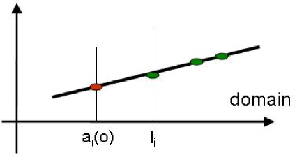
Figure 2: In a directional preference, the cost function is a monotone function of the attribute value. In the case shown here, smaller values are preferred.

A particular case of preferences in numeric domains is when the preference order can be assumed to have a known direction, such as for price (cheaper is always preferred, everything else being equal). In this case, $\delta(o_{1},o_{2})$ can be computed by simply comparing the values that the options take on that attribute (Figure 2).

$$\delta_{i}(o_{1},o_{2})\left\{\begin{array}[]{ll}\mbox{{\bf if} }a_{i}(o_{1})<a_{i}(o_{2})\mbox{ {\bf then} }1\mbox{ {\bf else} }0&\mbox{ }a_{i}\mbox{ numeric, natural preference }<\\ \mbox{{\bf if} }a_{i}(o_{1})>a_{i}(o_{2})\mbox{ {\bf then} }1\mbox{ {\bf else} }0&\mbox{ }a_{i}\mbox{ numeric, natural preference }>\\ \end{array}\right.$$ (10)

For a set of options $O^{\geq}$ whose values on $a_{i}$ lie between $l_{i}$ and $h_{i}$ we have

$$\delta_{i}(o,O^{\geq})\left\{\begin{array}[]{ll}1\,\mbox{ {\bf if} }a_{i}(o)<l_{i}\\ 0\,\mbox{ {\bf otherwise}}\\ \end{array}\right.$$ (13)

when smaller values are always preferred, and

$$\delta_{i}(o,O^{\geq})\left\{\begin{array}[]{ll}1\,\mbox{ {\bf if} }a_{i}(o)>h_{i}\\ 0\,\mbox{ {\bf otherwise}}\\ \end{array}\right.$$ (16)

when larger values are always preferred. Note that in both cases, the expressions are independent of the shape of the cost function as long as it is monotonic.

Threshold preferences in numeric domains

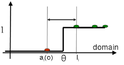
Figure 3: When the preference LessThan($\theta$) is represented by a step function, an option is preferred over a set of options with minimum value $l_{i}$ if the reference value $\theta$ falls in between the values of the given option and $l_{i}$.

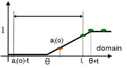
Figure 4: When the preference LessThan($\theta$) is represented by a graded step function, an option is preferred over a set of options with minimum value $l_{i}$ if the reference value $\theta$ falls in the interval between $a_{i}(o)-t$ and $l_{i}$, where $t=1/\alpha$.

Another commonly used preference expression in numeric domains is to define a smallest or largest acceptable threshold, i.e. to express a preference LessThan($\theta$) (the value should be lower than $\theta$) or GreaterThan($\theta$) (the value should be greater than $\theta$). Such a preference is most straightforwardly expressed by a cost function that follows a step curve (Figure 3). To express the fact that there is usually some tolerance for small violations, more generally a graded step function, where the cost gradually increases, might be used (Figure 4).

A possible cost function for LessThan might be the following:

$$c_{less-than}(\theta,x)=\left\{\begin{array}[]{ll}\mbox{Min}(1,\alpha*(x-\theta))&\mbox{ {\bf if} }x>\theta\\ 0&\mbox{{\bf otherwise}}\\ \end{array}\right.$$ (17)

assigning a penalty when the option takes a value greater than the reference value $\theta$; such cost is the difference between the value and the reference, up to a maximum of 1. $\alpha$ is a parameter that expresses the degree to which the violations can be allowed; for the following computations it is convenient to use the length of the ramp from 0 to 1 $t=1/\alpha$.

In this case the computation of $\delta(o_{1},o_{2})$ will be, if $a_{i}(o_{1})<a_{i}(o_{2})$:

$$\delta_{i}(o_{1},o_{2})=\int_{a_{i}(o_{1})-t}^{a_{i}(o_{2})}1p(\theta)d\theta=p[(a_{i}(o_{1})-t)<\theta<a_{i}(o_{2})];$$

and 0 otherwise (since lower values are preferred in Equation  17).

When the transition phase from 0 to 1 is small (the cost function approximates a step function as in Figure 3), $\delta_{i}(o_{1},o_{2})\simeq p[a_{i}(o_{1})-t<\theta<a_{i}(o_{2})]$, approximating the probability of the reference point falling between the two options. Assuming uniform distribution, the probability evaluates to $(a_{i}(o_{2})-a_{i}(o_{1})+t)/range(a_{i})$, where $range(a_{i})$ is that difference between the largest and smallest values of $a_{i}$. The reasoning is illustrated by Figure 4.

The probability computed is conditioned on the knowledge of the polarity of the user’s preference (LessThan in this case), and needs to be weighted by the probability of that polarity. Below, we assume that both polarities are equally likely, and use a weight of 1/2.

All the dominance relations can be broken simultaneously only if the considered option has a value for that attribute that is smaller or bigger than that of all the options in the dominating set. To estimate the probability that the reference value for the new preference falls in such a way that all the dominance relations are broken, it is sufficient to consider the extrema of the values that the dominating options take on the considered attribute:

• $h_{i}=max_{o^{\prime}\in O^{>}}a_{i}(o^{\prime})$

• $l_{i}=min_{o^{\prime}\in O^{>}}a_{i}(o^{\prime})$

If the values for the current option lies outside the interval $[l_{i},h_{i}]$, we can consider the probability of breaking all the relations as in the single dominance case. It will be proportional to the difference between the current option value and the minimum/maximum, scaled by the range of values for $a_{i}$:

$$\delta_{i}(o,O^{\geq})\left\{\begin{array}[]{ll}(a_{i}(o_{1})-h_{i}+t)/2*range(a_{i})&\mbox{if $a_{i}(o_{1})>h_{i}$ }\\ &\\ (l_{i}-a_{i}(o_{1})+t)/2*range(a_{i})&\mbox{if $a_{i}(o_{1})<l_{i}$ }\\ &\\ 0&\mbox{otherwise}\\ \end{array}\right.$$ (23)

Peaked preferences for numeric domains

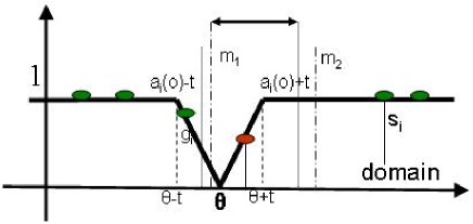
Figure 5: An example of peaked preferences. $g_{i}$ is the greatest value below $a_{i}(o)$ of $a_{i}$ for any option in $O^{\geq}(o)$, $s_{i}$ is the smallest value above $a_{i}(o)$. $m_{1}=(a_{i}(o)+g_{i})/2$, $m_{2}=(a_{i}(o)+s_{i})/2$ are the two midpoints between $a_{i}(o)$ and $g_{i}$, $s_{i}$. To make $o$ be preferred over all options in $O^{\geq}(o)$, $\theta$ has to fall between $max(m_{1},a_{i}(o)-t)$ and $min(m_{2},a_{i}(o)+t)$. As it can be seen graphically, in this case the interval is $]m_{1},a_{i}(o)+t[$.

Another common case is to have preferences for a particular numerical value $\theta$, for example “I prefer to arrive around 12am”. To allow some tolerance for deviation, a cost function might have a slope in both directions:

$$c_{peak}(x,\theta)=\alpha*|a_{i}(o)-\theta|.$$

In this case, an option is preferred to another one if it is closer to $\theta$. For example, letting $m$ be the midpoint between $a_{i}(o_{1})$ and $a_{i}(o_{2})$ and supposing $a_{i}(o_{1})<a_{i}(o_{2})$, we have

$$\delta(o_{1},o_{2})=p[\theta<m]$$

For calculating the probability of simultaneously breaking all the dominance relations without generating new ones, we define $g_{i}$ as the maximum of all dominating or equal options with a value for $a_{i}$ less than $a_{i}(o)$ and $s_{i}$ as the minimum value of all dominating or equal options greater than $a_{i}(o)$. As option $o$ is more preferred whenever $a_{i}(o)$ is closer to $\theta$, and the interval for $\theta$ where this is the case is one half the interval between $s_{i}$ and $g_{i}$, we have:

$$\delta(o,O^{\geq})=\frac{s_{i}-g_{i}}{range(a_{i})}$$

A more realistic cost function would include a “saturation point” from which the cost always evaluates to 1, as shown in Figure 5:

$$c_{peak-with-saturation}(x,\theta)=\mbox{Min}(1,\alpha*|a_{i}(o)-\theta|).$$ (24)

Let $t=1/\alpha$ be the tolerance of the preference to either side, $g_{i}$ be the greatest value below $a_{i}(o)$ of $a_{i}$ for any option in $O^{\geq}(o)$, and $s_{i}$ be the smallest value above $a_{i}(o)$. We define two midpoints $m_{1}=(a_{i}(o)+g_{i})/2$ and $m_{2}=(a_{i}(o)+s_{i})/2$, and we then have:

$$\delta(o,O^{\geq})=p[\mbox{max}(m_{1},a_{i}(o)-t)<\theta<\mbox{min}(m_{2},a_{i}(o)+t)]$$

If the reference point is uniformly distributed, this evaluates to:

$$\delta(o,O^{\geq})=\frac{\min(m_{2},a_{i}(o)+t)-\max(m_{1},a_{i}(o)-t)}{range(a_{i})}$$ (25)

3.4 Example

The following table shows the relevant values for the example shown earlier. Recall that we had earlier identified $o_{4}$ and $o_{3}$ as the most attractive suggestions.

	$O^{+}$	rent	type	$\delta_{2}$	distance	$\delta_{3}$	furnished	$\delta_{4}$	${\bf p_{opt}}$
		($a_{1}$)	($a_{2}$)		($a_{3}$)		($a_{4}$)
$o_{1}$	-	400	room	-	17	-	yes	-	-
$o_{2}$	$o_{1}$	500	room	0	32	0.25	yes	0	0.125
$o_{3}$	$o_{1},o_{2}$	600	apartment	0.5	14	0.05	no	0.5	0.451
$o_{4}$	$o_{1},o_{2}$	600	studio	0.5	5	0.20	no	0.5	0.494
$o_{5}$	$o_{1}-o_{4}$	650	apartment	0	32	0	no	0	0
$o_{6}$	$o_{1}-o_{5}$	700	studio	0	2	0.05	yes	0	0.025
$o_{7}$	$o_{1}-o_{6}$	800	apartment	0	7	0	no	0	0

In the counting strategy, options are ranked according to the size of the set $O^{+}$. Thus, we have $o_{2}$ as the highest ranked suggestion, followed by $o_{3}$ and $o_{4}$.

In the probabilistic strategy, attribute values of an option are compared with the range of values present in its dominators. For each attribute, this leads to the $\delta$ values as indicated in the table. If we assume that the user is equally likely to have a preference on each attribute, with a probability of $P_{a_{i}}=0.5$, the probabilistic strategy scores the options as shown in the last column of the table. Clearly, $o_{4}$ is the best suggestion, followed by $o_{3}$. $o_{2}$ and also $o_{6}$ follow further behind.

Thus, at least in this example, the model-based strategies are successful at identifying good suggestions.

3.5 Optimizing a Set of Several Suggestions

The strategies discussed so far only concern generating single suggestions. However, in practice it is often possible to show a set of $l$ suggestions simultaneously. Suggestions are interdependent, and it is likely that we can obtain better results by choosing suggestions in a diverse way. This need for diversity has also been observed by others (?, ?).

More precisely, we should choose a group $G$ of suggested options by maximizing the probability $p_{opt}(G)$ that at least one of the suggestions in the set $G$ will become optimal through a new user preference:

$$p_{opt}(G)=1-\prod_{a_{i}\in A_{u}}(1-P_{a_{i}}(1-\prod_{o^{\prime}\in G}(1-\delta_{i}(o^{\prime},O^{\geq}(o^{\prime})))))$$ (26)

Explicitly optimizing this measure would lead to combinatorial complexity. Thus, we use an algorithm that adds suggestions one by one in the order of their contribution to this measure given the already chosen suggestions. This is similar to the algorithm used by Smyth and McClave (?) and by Hebrard et al. (?) to generate diverse solutions.

The algorithm first chooses the best single suggestion as the first element of the set $G$. It then evaluates each option $o$ as to how much it would change the combined measure $p_{opt}(G)$ if it were added to the current $G$, and adds the option with the largest increment. This process repeats until the desired size of set $G$ is reached.

3.6 Complexity

Let $n$ be the number of options, $k$ the number of attributes and $m$ the number of preferences, $d$ the number of dominators, $A_{u}$ the attributes on which the user did not state any preference.

All three model-based strategies are based on the dominating set of an option. We use a straightforward algorithm that computes this as the intersection of the set of options that are better with respect to individual preferences. There are $m$ such sets, each with at most $n$ elements, so the complexity of this algorithm is $O(n^{2}m)$. In general, the dominating set of each option is of size $O(n)$ so that the output of this procedure is of size $O(n^{2})$, so it is unlikely that we can find a much better algorithm.

Once the dominating sets are known, the counting strategy has complexity $O(nd)$, while the attribute and probabilistic strategies have complexity $O(ndk_{u})$, where $k_{u}=|A_{u}|$ and $k_{u}<k$. In general, $d$ depends on the data-set. In the worst case it can be proportional to $n$, so the resulting complexity is $O(n^{2})$.

When utility is used as a domination criterion, the dominating set is composed by the options that are higher in the ranking. Therefore the process of computing the dominating set is highly simplified and can be performed while computing the candidates. However the algorithm still has overall worst case complexity $O(n^{2})$: the the last option in the ranking has $n-1$ dominators, and so $d=O(n)$.

When several examples are selected according to their diversity, the complexity increases since the metrics must be recomputed after selecting each suggestion.

In comparison, consider the extreme strategy, proposed initially by Linden et al. in ATA (?). It selects options that have either the smallest or the largest value for an attribute on which the user did not initially state any preference. This strategy needs to scan through all available options once. Its complexity is $O(n)$, where $n$ is the number of options (the size of the catalog). Thus, it is significantly more efficient, but does not appear to provide the same benefits as a model-based strategy, as we shall see in the experiments.

Another strategy considered for comparison, that of generating a maximally diverse set of options (?, ?), has an exponential complexity for the number of available options. However, greedy approximations (?) have a complexity of only $O(n^{2})$ , similar to our model-based strategies.

The greedy algorithm we use for optimizing a set of several suggestions does not add to the complexity; once the distances $\delta_{i}$ have been computed for each attribute, the greedy algorithm for computing the set of suggestions has a complexity proportional to the product of the number of options, the number of attributes, and the square of the number of suggestions to be computed. We suspect that an exact optimization would be NP-hard in the number of suggestions, but we do not have a proof of this.

4 Experimental Results: Simulations

Figure 6: Simulation results on a database of actual apartment offers. For 100 simulated users, each with a randomly chosen preference model of 6 hidden preferences, we plot the number of times that the simulation discovered at least the number of preferences shown on the abscissa. The higher the curve, the more preferences were discovered on average.

Figure 7: Simulation results for randomly generated catalogs. For 100 simulated users, each with a randomly chosen preference model of 8 hidden preferences, we plot the number of times that the simulation discovered at least the number of preferences shown on the abscissa. The higher the curve, the more preferences were discovered on average.

The suggestion strategies we presented are heuristic, and it is not clear which of them performs best under the assumptions underlying their design. Since evaluations with real users can only be carried out for a specific design, we first select the best suggestion strategy by simulating the interaction of a computer generated user with randomly generated preferences. This allows us to compare the different techniques in much greater detail than would be possible in an actual user study, and thus select the most promising techniques for further development. This is followed by real user studies that are discussed in the next section.

In the simulations, users have a randomly generated set of $m$ preferences on the different attributes of items stored in a database. As a measure of accuracy, we are interested in whether the interaction allows the system to obtain a complete model of the user’s preferences. This tests the design objective of the suggestion strategies (to motivate the user to express as many preferences as possible) given that the assumptions about user behavior hold. We verify that these assumptions are reasonable in the study with real users reported in the next section.

The simulation starts by assigning the user a set of randomly generated preferences and selecting one of them as an initial preference. At each stage of the interaction, the simulated user is presented with 5 suggestions.

We implemented 6 different strategies for suggestions, including the three model-based strategies described above as well as the following three strategies for comparison:

• the random strategy suggests randomly chosen options;

• the extremes strategy suggests options where attributes take extreme values, as proposed by Linden (?);

• the diversity strategy computes the 20 best solutions according to the current model and then generates a maximally diverse set of 5 of them, following the proposal of McSherry (?).

The simulated user behaves according to an opportunistic model by stating one of its hidden preferences whenever the suggestions contain an option that would become optimal if that preference was added to the model with the proper weight. The interaction continues until either the preference model is complete, or the simulated user states no further preference. Note that when the complete preference model is discovered, the user finds the target option.

We first ran a simulation on a catalog of student accommodations with 160 options described using 10 attributes. The simulated user was shown 5 suggestions, and had a randomly generated model of 7 preferences, of which one is given by the user initially. The results are shown in Figure 6. For each value of x, it shows the percentage of runs (out of 100) that discover at least x out of the 6 hidden preferences in the complete model. Using random suggestions as the baseline, we see that the extremes strategy performs only slightly better, while diversity provides a significant improvement. The model-based strategies give the best results, with the counting strategy being about equally good as diversity, and the probabilistic strategies providing markedly better results.

In another test, we ran the same simulation for a catalog of 50 randomly generated options with 9 attributes, and a random preference model of 9 preferences, of which one is known initially. The results are shown in Figure 7. We can see that there is now a much more pronounced difference between model-based and non model-based strategies. We attribute this to the fact that attributes are less correlated, and thus the extreme and diversity filters tend to produce solutions that are too scattered in the space of possibilities. Also the probabilistic strategy with both possible implementations (assuming the attributes values independent or not) give very close results.

#P / #A	random	extreme	diversity	counting	prob1	prob2
6/6	0.12	0.09	0.23	0.57	0.59	0.64
6/9	0.12	0.12	0.27	0.65	0.63	0.67
6/12	0.11	0.13	0.24	0.62	0.64	0.63

Table 1: The fraction of preferences that are correctly discovered as a function of the number of attributes; keeping constant the number of preferences (6) to be discovered. All attributes have integer domains.

#P / #A	random	extreme	diversity	counting	prob1	prob2
3/9	0.25	0.36	0.28	0.70	0.71	0.71
6/9	0.11	0.12	0.11	0.67	0.68	0.68
9/9	0.041	0.17	0.05	0.66	0.70	0.73

Table 2: The fraction of preferences that are correctly discovered (on average) as a function of the number of preferences to be discovered. All attributes have integer domains.

We investigated the impact of the number of preferences, the number and type of attributes, and the size of the data set on random data sets. In the following, prob1 refers to the probabilistic strategy with the independence assumption, prob2 to the probabilistic strategy without that assumption.

Surprisingly we discovered that varying the number of attributes only slightly changes the results. Keeping the number of preferences constant at 6 (one being the initial preference), we ran simulations with the number of attributes equal to 6, 9 and 12. The average fraction of discovered preferences varied for each strategy and simulation scenario by no more than $5\%$, as shown in Table 1.

domain	random	extreme	diversity	counting	prob1	prob2
type	choice
mixed	0.048	0.30	0.18	0.81	0.87	0.86
integer	0.04	0.17	0.05	0.66	0.70	0.72

Table 3: The fraction of preferences that are correctly discovered as a function of the different kinds of attribute domains: integer domains against a mix of 5 integer, 2 discrete domains and 2 domains with a natural order. We ran 100 simulations with 9 attributes and 9 preferences.

data	random	extreme	diversity	counting	prob1	prob2
size	choice
50	0.25	0.50	0.56	0.89	0.94	0.93
75	0.16	0.42	0.54	0.88	0.97	0.95
100	0.11	0.29	0.57	0.90	0.96	0.97
200	0.05	0.22	0.54	0.86	0.91	0.93

Table 4: The fraction of preferences that are correctly discovered as a function of the database size. We ran 100 simulations with 9 attributes and 9 preferences (mixed domains).

The impact of the variation of the number of preferences to discover is shown in Table 2. All of our model-based strategies perform significatively better than random choice, suggestions of extrema, and maximization of diversity. This shows the importance of considering the already known preferences when selecting suggestions.

The performances are higher with mixed domains than with all numeric domains (Table 3). This is easily explained by the larger outcome space in the second case.

Interestingly, as the size of the item set grows, the performance of random and extreme strategies significantly degrades while the model-based strategies maintain about the same performance (Table 4).

In all simulations, it appears that the probabilistic suggestion strategy is the best of all, sometimes by a significant margin. We thus chose to evaluate this strategy in a real user study.

5 Experimental Results: User Study

The strategies we have developed so far depend on many assumptions about user behavior and can only be truly tested by evaluating them on real users. However, because of the many factors that influence user behavior, only testing very general hypotheses is possible. Here, we are interested in verifying that:

1. using model-based suggestions leads to more complete preference models.

2. using model-based suggestions leads to more accurate decisions.

3. more complete preference models tend to give more accurate decisions, so that the reasoning underlying the model-based suggestions is correct.

We measure decision accuracy as the percentage of users that find their most preferred choice using the tool. The most preferred choice was determined by having the subjects go through the entire database of offers in detail after they finished using the tool. This measure of decision accuracy, also called the switching rate, is the commonly accepted measure in marketing science (e.g., ?).

We performed user studies using FlatFinder, a web application for finding student housing that uses actual offers from a university database that is updated daily. This database was ideal because it contains a high enough number - about 200 - of offers to present a real search problem, while at the same time being small enough that it is feasible to go through the entire list and determine the best choice in less than 1 hour. We recruited student subjects who had an interest in finding housing and thus were quite motivated to perform the task accurately.

We studied two settings:

• in an unsupervised setting, we monitored user behavior on a publicly accessible example-critiquing search tool for the listing. This allowed us to obtain data from over a hundred different users; however, it was not possible to judge decision accuracy since we were not able to interview the users themselves.

• in a supervised setting, we had 40 volunteer students use the tool under supervision. Here, we could determine decision accuracy by asking the subjects to carefully examine the entire database of offers to determine their target option at the end of the procedure. Thus, we could determine the switching rate and measure decision accuracy.

There are 10 attributes: type of accommodation (room in a family house, room in a shared apartment, studio apartment, apartment), rent, number of rooms, furnished (or not), type of bathroom (private or shared), type of kitchen (shared, private), transportation available (none, bus, subway, commuter train), distance to the university and distance to the town center.

For numerical attributes, a preference consists of a relational operator (less than, equal, greater than), a threshold value and an importance weight between 1-5; for example, ”price less than 600 Francs” with importance 4. For qualitative attributes, a preference specifies that a certain value is preferred with a certain importance value. Preferences are combined by summing their weights whenever the preference is satisfied, and options are ordered so that the highest value is the most preferred.

Users start by stating a set $P_{I}$ of initial preferences, and then they obtain options by pressing a search button. Subsequently, they go through a sequence of interaction cycles where they refine their preferences by critiquing the displayed examples. The system maintains their current set of preferences, and the user can state additional preferences, change the reference value of existing preferences, or even remove one or more of the preferences. Finally, the process finishes with a final set of preferences $P_{F}$, and the user chooses one of the displayed examples.

The increment of preferences $\mid P_{F}-P_{I}\mid$ is the number of extra preferences stated and represents the degree to which the process stimulates preference expression.

The search tool was made available in two versions:

• C, only showing a set of 6 candidate apartments without suggestions, and

• C+S, showing a set of 3 candidate apartments and 3 suggestions selected according to the probabilistic strategy with a utility-dominance criterion.

We now describe the results of the two experiments.

5.1 Online User Study

tool without suggestions tool with suggestions number of critiquing cycles 2.89 3.00 initial preferences 2.39 2.23 final preferences 3.04 3.69 increment 0.64 1.46

Table 5: Average behavior of users of the on-line experiment. We collected logs of real users looking for a student accommodation with our tool, hosted on the laboratory website.

FlatFinder has been hosted on the laboratory web-server and made accessible to students looking for accommodation during the winter of 2004-2005. For each user, it anonymously recorded a log of the interactions for later analysis. The server presented users with alternate versions of the system, i.e. with (C+S) and without (C) suggestions. We collected logs from 63 active users who went through several cycles of preference revision.

In analyzing the results of these experiments, whenever we present a hypothesis comparing users of the same group, we show its statistical significance using a paired test. For all hypotheses comparing users of different groups, we use the impaired student test to indicate statistical significance. In both cases, we indicate significance by p, the probability of obtaining the observed data under the condition that the null hypothesis is true. Values of p $<$ 0.05 are considered significant, p $<$ 0.01 highly significant and p $<$ 0.001 very highly significant.

We first considered the increment from initial preference enumeration $\mid P_{I}\mid$ to final preference enumeration $\mid P_{F}\mid$, as shown in Table 5. This increment was on average 1.46 for the tool with suggestions C+S and only 0.64 for the tool C ($128\%$ increase), showing the higher involvement of users when they see suggestions. This hypothesis was confirmed with p = 0.002.

It is interesting to see that in both groups the users interacted for a similar number of cycles (average of 2.89 and 3.00; p = 0.42, the null hypothesis cannot be rejected), and that the number of initial preferences is also close (average of 2.39 and 2.23, null hypothesis cannot be rejected with p = 0.37), meaning that the groups are relatively unbiased.

The result of the test (Table 5) shows clearly that users are more likely to state preferences when suggestions are present, thus verifying Hypothesis 1. However, as this is an online experiment, we are not able to measure decision accuracy. In order to obtain these measures, we also conducted a supervised user study.

5.2 Supervised User study

Characteristics		Participants
Gender	Male	31
	Female	9
Age	10s	2
	20s	36
	30s	2
Education	Undergraduate	36
	Phd	4
Familiar with online apartment search
	Yes	26
	No	14
Familiar with apartments in the area
	Yes	27
	No	13

Table 6: Demographic characteristics of participants for the supervised user study.

		Interaction with	Interaction with
		first interface	second interface
group 1	Tool version	C	C+S
(C first)	Decision Accuracy (mean)	0.45	0.80
	Preference Enumeration (mean)	5.30	6.15
	Interaction cycles (mean)	5.60	4.55
	Interaction time (min.,mean)	8:09	4.33
group 2	Tool version	C+S	C
(C+S first)	Decision Accuracy (mean)	0.72	0.67
	Preference Enumeration (mean)	5.44	4.50
	Interaction cycles (mean)	4.05	6.25
	Interaction time (mean)	7.39	3.33

Table 7: Results for the supervised experiment. Decision accuracy and preference enumeration (the number of preferences stated) are higher when suggestions are provided (interface C+S, showing 3 candidates and 3 suggestions) rather than when suggestions are not provided (interface C, 6 candidates).

The supervised user study used the same tool as the online user study but users were followed during their interaction.

To measure improvement of accuracy, we instructed all of the users to identify their most preferred item by searching the database using interface 1. This choice was recorded and was called $c_{1}$. Then the users were instructed to interact with the database using interface 2 and indicate a new choice ($c_{2}$) if the latter was an improvement on $c_{1}$ in their opinion. To evaluate whether the second choice was better than the initial one, we instructed the users to review all apartments (100 apartments in this case) and tell us whether $c_{1}$, $c_{2}$, or a completely different one truly seemed best.

Thus, the experiment allowed us to measure decision accuracy, since we obtained the true target choice for each user. If users stood by their first choice, it indicated that they had found their target choice without further help from the second interface. If users stood by their second choice, it indicated that they had found their target choice with the help of the second interface. If users chose yet another item, it indicated that they had not found their target choice even though they performed search with both interfaces.

40 subjects, mostly undergraduate students, with 9 different nationalities took part in the study. Most of them (27 out of 40) had searched for an apartment in the area before and had used online sites (26 out of 40) to look for accommodations. Table 6 shows some of their demographic characteristics. The subjects were motivated by the interest of finding a better apartment for themselves, which meant that they treated the study seriously.

To overcome bias due to learning and fatigue, we divided the users in two groups, who were asked to interact with the versions in two different orders:

• group $1$ used tool C (step 1) and then C+S (step 2)

• group $2$ used tool C+S (step 1) and then C (step 2)

Both groups then examined the entire list to find the true most preferred option. For each version of the tool and each group, we recorded the fraction of subjects where the final choice made using that interface was equal to the target option as decision accuracy. For both groups, we refer to accuracy of interface 1 as $acc_{1}$, and accuracy of interface 2 as $acc_{2}$.

We expected that the order of presenting the versions would be important. Once the users realized their own preferences and found a satisfactory option, they are likely to be consistent with that. Therefore, we expected $acc_{2}>acc_{1}$ in both cases. However, we expected that average accuracy would significantly increase with suggestions, and so the results would show $acc_{2}>>acc_{1}$ in the first group and $acc_{2}$ only slightly higher than $acc_{1}$ in group 2.

Table 7 shows the results. In the next section we want to verify Hypothesis 2 (decision accuracy improves with suggestions) and 3 (preference enumeration improves accuracy). Finally we will check whether a mediation phenomenon is present (meaning that the improvement of accuracy is entirely explained by the fact that suggestions lead to an increase of preferences).

Decision Accuracy improves with suggestions

   

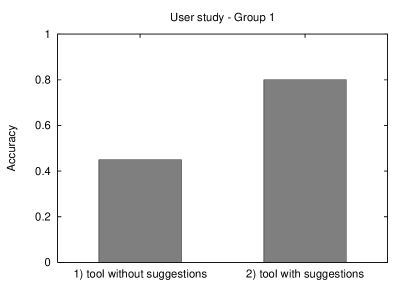
(a) For group 1, accuracy dramatically increased when they used the version with suggestions (C+S).

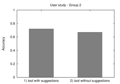
(b) For group 2, accuracy is already very high when they use the version with suggestions (C+S). Further interaction cycles with the tool C showing 6 candidates does not increase accuracy any further.

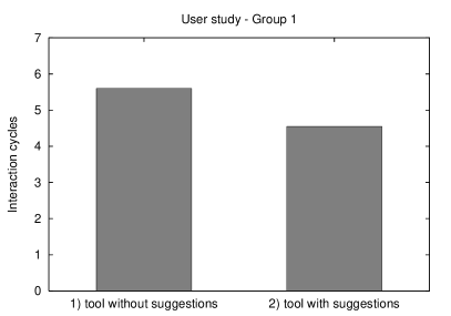
(c) For group 1, users needed less interaction cycles to make a choice when using the interface with suggestions (C+S).

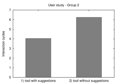
(d) For group 2, the number of interaction cycles significantly increased when they used the version without suggestions (C).

Figure 8: Decision accuracy and interaction cycles for both groups of users of the supervised experiment.

Figure 8 shows the variation of decision accuracy and the number of interaction cycles for the two groups.

For group 1, after interaction with tool C, the average accuracy is only 45%, but after interaction with C+S, the version with suggestions, it goes up to 80%. This confirms the hypothesis that suggestions improve accuracy with p = 0.00076. 10 of the 20 subjects in this group switched to another choice between the two versions, and 8 of them reported that the new choice was better. Clearly, the use of suggestions significantly improved decision accuracy for this group.

Users of group 2 used C+S straight away and achieved an average accuracy of 72% at the outset. We expected that a consequent use of tool $C$ would have a small positive effect on the accuracy, but in reality the accuracy decreased to 67%. 10 subjects changed their final choice using the tool without suggestions, and 6 of them said that the newly chosen was only equally good as the one they originally chose. The fact that accuracy does not drop significantly in this case is not surprising because users remember their preferences from using the tool with suggestions and will thus state them more accurately independently of the tool. We can conclude from this group that improved accuracy is not simply the result of performing the search a second time, but due to the provision of suggestions in the tool. Also, the closeness of the accuracy levels reached by both groups when using suggestions can be interpreted as confirmation of its significance.

We also note that users of interface C+S needed fewer cycles (and thus less effort) to make decisions (average of 4.15) than interface C (5.92).

Interestingly, the price of the chosen apartment increased for the first group (average of 586.75 for C to 612.50 for C+S; p = 0.04, statistically significant), whereas it decreased for the second group (average of 527.20 for C+S to 477.25 for C; p = 0.18, the decrease is not statically significant). We believe that subjects in the first group did not find a good choice, and thus paid a relatively high price to get an apartment with which they would feel comfortable. Conditioned on this high price, they were then willing to spend even more as they discovered more interesting features through suggestions. On the other hand, subjects in group 2 already found a good choice in the first use of the tool, and were unwilling to accept a high price when they did not find a better choice in the second search without suggestions.

Thus, we conclude that Hypothesis 2 is confirmed: suggestions indeed increase decision accuracy.

Preference enumeration improves accuracy

In this study, we notice that when suggestions are present, users state a higher number of preferences (average of 5.8 preferences vs. only 4.8 without suggestions, p = 0.021), so that Hypothesis 1 is again confirmed.

To validate hypothesis 3, that a higher preference enumeration also leads to more accurate decisions, we can compare the average size of the preference model for those users who found their target solution with the first use of the tool and those who did not. In both groups, users who did find their target in the first try stated on average 5.56 preferences (5.56 in group 1 and 5.57 in group 2) while users who did not find their target stated only an average of 4.88 preferences (5.09 in group 1 and 4.67 in group 2). This shows that increased preference enumeration indeed improves accuracy but unfortunately we did not find this statistically significant (p = 0.17). In fact, there is a chance that this correlation is due to some users being more informed and thus making more accurate decisions and stating more preferences.

found	0.45	0.83
still not found	0.55	0.17
	$\Delta|P|<=0$	$\Delta|P|>0$

Table 8: For users who did not find their target in the first use of the tool, the table shows the fraction that did and did not find their target in the next try, depending on whether the size of their preference model did or did not increase. ($\Delta|P|$ is the variation of the number of stated preferences $|P|$ between the two uses of the tool).

As an evaluation independent of user’s a priori knowledge, we considered those users who did not find their target in the first try only. As a measure of correlation of preference enumeration and accuracy, we considered how often an increase in preference enumeration in the second try led to finding the most preferred option on the second try. Table 8 shows that among users whose preference model did not grow in size, only $45\%$ found their target, whereas of those that increased their preference model, $83\%$ found their target. Again, we see a significant confirmation that higher preference enumeration leads to a more accurate decision with real users (p = 0.038251).

$\Delta acc>0$	0.23	0.14	0.38
$\Delta acc=0$	0.62	0.71	0.62
$\Delta acc<0$	0.15	0.14	0.00
	$\Delta|P|<0$	$\Delta|P|=0$	$\Delta|P|>0$

Table 9: Variation of accuracy against variation of the number of stated preferences $|P|$ between the two uses of the tool.

Finally, a third confirmation can be obtained by considering the influence that variations in the size of the preference model have on decision accuracy, shown in Table 9. Each column corresponds to users where the size of the preference model decreased, stayed the same, or increased. It also shows the fraction for which the accuracy increased, stayed the same or decreased (note that when accuracy is 1 at the first step, it cannot further increase). We can see that a significant increase in accuracy occurs only when the size of the preference model increases. In all other cases there are some random variations but no major increases. The statistical test shows that the hypothesis that an increase in preference enumeration causes an increase in accuracy is confirmed with p = 0.0322.

Thus, we conclude that hypothesis 3 is also validated by the user study; a more complete preference model indeed leads to more accurate decisions.

Mediation analysis

Since our three hypotheses are verified, the presence of suggestions lead to an increase of the preferences stated and consequently to an increase in accuracy. With a 3-step mediation analysis we want to check whether there is a mediation phenomenon, meaning that the increase of accuracy is entirely explained by the increase of the preferences.

However, a Sobel test did not show statistical significance (p=0.14), so we cannot conclude that the increase of the preference enumeration is a “mediator”. Our interpretation is that suggestions influence decision accuracy by also making the users state better preferences.

5.3 Other Observations

A more objective measure of confidence is the price that people are willing to pay for the chosen option as a measure of their satisfaction, since they would only pay more if the choice satisfies them more based on the other attributes. For the 40 subjects, the average rent of the chosen housing with suggestion was CHF 569.85, an increase of about $7\%$ from the average without suggestions, which was CHF532.00. In fact, we can observe a general correlation between price and accuracy, as 9 out of the 10 subjects that did not find their target in the first interaction finally chose an apartment with higher rent.

All subjects notably liked the interaction (average 4.1 out of 5) with no significant difference between the versions. We asked the subjects which version they considered more productive. The majority of them, 22 out of 40, preferred the version with suggestions, while 13 preferred the version with more candidates and 5 had no opinion.

Another indication that suggestions are helpful is the average time to complete the decision task: while it took subjects an average of 8:09 minutes to find their target without suggestions, the version with suggestions took only 7:39 minutes on average. Thus, using suggestions users take less time but obtain a more accurate decision.

6 Related Work

Example-based search tools

Burke and others (?) have been among the first to recognize the challenge of developing intelligent tools for preference-based search. Their approach, called assisted browsing combines searching and browsing with knowledge based assistance and recognizes that users are an integral part of the search process.

They developed the FindMe approach, consisting of a family of prototypes that implement the same intuition in a variety of domains (restaurants, apartments, cars, video, etc.). The main features are the possibility of similarity based retrieval (look for a restaurant similar to this, but in San Francisco), the support for tweaking (look for bigger, nicer, closer to centre, ..), abstraction of high level features (users might look for a restaurant with casual look, where look is not defined in the database directly, but decoupled into a few basic features), and multiple similarity metrics. The display follows a hierarchical sort where the preferences (described by goals: minimize price, find a seafood cuisine) have a fixed priority. The restaurant advisor was tested on-line for several years.

Another early and similar work is the ATA system of Linden et al. (?). ATA is a tool for planning travel itineraries based on user’s constraints. It followed the so-called candidate-critiquing cycle where users could post constraints on their travel and would be shown the 3 best matching flights from the database. ATA was tested on-line for several months.

In more recent work, Shearin and Lieberman (?), have described AptDecision, an example-critiquing interface where the user is able to guide the search by giving feedback on any feature (in the form of either positive or negative weights) at any time. All of these critiques are stored in a profile that is displayed at the bottom part of the interface and can be modified or stored for later use. Instead of providing feedback manually, the user might prefer to let AptDecision learn his or her profile weights by comparing two sample examples. However, they did not investigate strategies for suggestions.

Improving example selection

Techniques to induce users to state their preferences more accurately have been proposed in various recommender systems. Suggestion mechanisms include extreme values, diversity, and compound critiques.

The ATA system of Linden et al. (?) included a suggestion strategy of showing extreme examples applied to the airplane travel domain, for example the first and last flight of the day. In our simulations, we compared our model-based techniques to this strategy.

Several researchers (?, ?, ?, ?, ?, ?) have studied the issue of achieving a good compromise between generating similar and diverse results in case-based retrieval. They consider the problem of finding cases that are most similar to a given query case, but at the same time maximize the diversity of the options proposed to the user. Smyth et. al (?) improves the common query show me more like this: their adaptive search algorithm alternates between a strategy that privileges similarity and one that privileges diversity (refocus). McSherry (?) took this idea further and provided selection algorithms that maximize diversity and similarity at the same time. McSherry (?) proposes a technique where retrieved cases are associated with a set of like cases that share identical differences with the query case. The like cases are not displayed among the examples, but accessible to users on demand. Thus, the retrieval set can be more diverse.

Reilly et al. (?) also uses a mixture of similarity and diversity, with the goal of providing possible standardized critiques to allow trade-offs analysis in an e-commerce environment. A critique is, in this scope, a modification of a user’s current preferences for narrowing down the search or it is an indication of a trade-off. Users can select either unit critiques which revise preferences on individual attributes, or compound critiques which revise preferences on multiple attributes. The compound critiques are organized into categories and displayed in natural language form, for example more memory and larger and heavier. One of the innovations in their work is the automatic generation of sensible critiques involving several features based on available items using the Apriori algorithm. Both simulated and real user studies have shown that compound critiques significantly reduce the number of interaction cycles.

All of these approaches, however, differ from ours in the sense that they do not have an explicit preference model. The recent work of Hebrard et al. (?) has investigated the computational problem of generating diverse solutions to constraint satisfaction problems.

Dialogue-based approaches

Many other related works try to simulate human conversation in order to guide the customer through the decision making process. Shimazu (?) describes ExpertClerk, an agent system that imitates a human salesclerk. In the first phase, the agent tries to narrow down the possibilities by asking questions. An optimal discrimination tree is built using information gain (as in ID3 algorithm) where each node represents a specific question to the user, and the user’s answer leads into a specific portion of the subtree. In fact, each node is equivalent to a crisp constraint, and the problem of getting to a node with no compatible examples may occur. In the second phase, the agent proposes three possible items, chosen to be one in the central and two in the opposite extreme region of the available product space. It is shown that an intelligent use of both strategies (asking and proposing) is more efficient that one of the two strategies alone.

? (?) also propose a conversational, dialogue-based approach in ADAPTIVE PLACE ADVISOR, a conversational recommendation system for restaurants in the Palo Alto area. Their approach mimics a conversation that proceeds with questions like What type of food would you like?; the user might either answer with a particular answer like Chinese, say that he or she does not care about this aspect, or ask the advisor about the possible choices. User preferences obtained during the current conversation are treated as crisp constraints and only items that satisfy them are considered. When there are no items that satisfy all preferences, the system may ask the user whether he or she is willing to relax some constraints.

The tool also develops a long-term user model that keeps track of preferences expressed in previous interactions. It is used to sort the results that are shown to the user.

Using prior knowledge

It is also possible to optimize the set of examples given an expectation of the user’s preferences, without actually asking the users to state their own preferences. This is the approach described by Price and Messinger (?). This work differs from ours in that they do not consider preferences of an individual user, but average preferences for a group of users.

Preference elicitation can be optimized using prior distributions of possible preferences. This approach was proposed by Chajewska et al. (?) to produce a more efficient preference elicitation procedure. The elicitation is a question-answering interaction where the questions are selected to maximize the expected value of information. Boutilier (?) has extended this work by taking into account values of future questions to further optimize decision quality while minimizing user effort. He views the elicitation procedure itself as a decision process and uses observable Markov process (POMDP) to obtain an elicitation strategy.

Such approaches require that users are familiar enough with the available options to answer any question about value functions without the benefit of example outcomes to assess them. In contrast, in a mixed-initiative system as described here the user is free to furnish only the information she is confident about. It is also questionable whether one can assume a prior distribution on preferences in personalized recommendation systems where users may be very diverse.

7 Conclusion

We considered AI techniques used for product search and recommender systems based on a set of preferences explicitly stated by users. One of the challenges recognized in this field is the elicitation of an accurate preference model from each user. In particular, we face the dilemma of accuracy at the cost of user effort.

Some systems may introduce severe errors into the model because users cannot expend the amount of effort required to state preferences, while others may require little effort but provide very general recommendations because the preference model was never completely established. The ideal solution is one that provides users with accurate recommendations while minimizing their effort in stating preferences. Therefore, this article also examined user interaction issues and emphasized models that motivate users to state more complete and accurate preferences, while requiring the least amount of effort from the user.

We conjectured that the benefit of discovering attractive recommendations presents a strong motivation for users to state additional preferences. Thus, we developed a model-based approach that analyzes the user’s current preference model and potential hidden preferences in order to generate a set of suggestions that would be attractive to a rational user. This suggestion set is calculated based on the look-ahead principle: a good suggestion is an outcome that becomes optimal when additional hidden preferences have been considered. Through simulations, we demonstrated the superior performance of these model-based strategies in comparison to the other proposed strategies.

We further validated our hypothesis that such strategies are highly likely to stimulate users to express more preferences through a significant within-subject user study involving 40 real users. We measured decision accuracy, defined as the percentage of users who actually found their most preferred option with the tool, for an example-critiquing tool with and without suggestions.

The study showed that users are able to achieve a significantly higher level of decision accuracy with an example-critiquing tool with suggestions than without suggestions, increasing from 45 to 80$\%$, while the effort spent on both tools is comparable. This shows that there is significant potential for improving the tools that are currently in use.

It is important to note that this performance is obtained with users who are not bound to a particular dialogue, but are free to interact with the system on their own initiative.

This process particularly supports preference expression for users who are unfamiliar with the domain, and typically for decisions which require low to medium financial commitments. For highly important decisions where users understand their preferences well, other preference elicitation techniques (?, ?) are likely to provide superior results.

As the strategies are based on the very general notion of Pareto-optimality, they can be applied to a broad range of preference modeling formalisms, including utility functions, soft constraints  (?), and CP-networks  (?). This will greatly strengthen the performance of example-critiquing systems in applications ranging from decision support to e-commerce.

8 Acknowledgements

The authors would like to thank Vincent Schickel-Zuber for his significant contribution in the development of the web based interface for FlatFinder, and Jennifer Graetzel for her insightful suggestions on the various draft versions of this manuscript to improve its readability. This work was supported by the Swiss National Science Foundation under contract No. 200020-103421.

References

- Adomavicius and Tuzhilin Adomavicius, G., and Tuzhilin, A. (2005). Toward the next generation of recommender systems: A survey of the state-of-the-art and possible extensions. IEEE Transactions on Knowledge and Data Engineering, 17(6), 734–749.
- Bistarelli, Montanari, and Rossi Bistarelli, S., Montanari, U., and Rossi, F. (1997). Semiring-based constraint satisfaction and optimization. Journal of ACM, 44(2), 201–236.
- Boutilier Boutilier, C. (2002). A pomdp formulation of preference elicitation problems. In Proceedings of the Eighteenth National Conference on Artificial Intelligence (AAAI’02), pp. 239–246.
- Boutilier, Brafman, Domshlak, Hoos, and Poole Boutilier, C., Brafman, R. I., Domshlak, C., Hoos, H. H., and Poole, D. (2004). CP-nets: A tool for representing and reasoning with conditional ceteris paribus preference statements. Journal of Artificial Intelligence Research, 21, 135–191.
- Boutilier, Patrascu, Poupart, and Schuurmans Boutilier, C., Patrascu, R., Poupart, P., and Schuurmans, D. (2005). Regret-based utility elicitation in constraint-based decision problems.. In Proceedings of the Nineteenth International Joint Conference on Artificial Intelligence (IJCAI’05), pp. 929–934.
- Bridge and Ferguson Bridge, D. G., and Ferguson, A. (2002). Diverse product recommendations using an expressive language for case retrieval. In Proceedings of the 6th European Conference on Advances in Case-Based Reasoning (ECCBR’02), pp. 43–57.
- Burke Burke, R. (2002a). Interactive critiquing for catalog navigation in e-commerce. Artificial Intelligence Review, 18(3-4), 245–267.
- Burke Burke, R. D. (2002b). Hybrid recommender systems: Survey and experiments. User Model. User-Adapt. Interact., 12(4), 331–370.
- Burke, Hammond, and Young Burke, R. D., Hammond, K. J., and Young, B. C. (1997). The FindMe approach to assisted browsing. IEEE Expert, 12(4), 32–40.
- Chajewska, Koller, and Parr Chajewska, U., Koller, D., and Parr, R. (2000). Making rational decisions using adaptive utility elicitation. In Proceedings of the Seventeenth National Conference on Artificial Intelligence and Twelfth Conference on Innovative Applications of Artificial Intelligence (AAAI’00), pp. 363–369. AAAI Press / The MIT Press.
- Chomicki Chomicki, J. (2003). Preference formulas in relational queries. ACM Trans. Database Syst., 28(4), 427–466.
- Faltings, Torrens, and Pu Faltings, B., Torrens, M., and Pu, P. (2004). Solution generation with qualitative models of preferences. In Computational Intelligence, pp. 246–263(18). ACM.
- Haubl and Trifts Haubl, G., and Trifts, V. (2000). Consumer decision making in online shopping environments: The effects of interactive decision aids. Marketing Science, 19(1), 4–21.
- Hebrard, Hnich, O’Sullivan, and Walsh Hebrard, E., Hnich, B., O’Sullivan, B., and Walsh, T. (2005). Finding diverse and similar solutions in constraint programming. In Proceedings of the Twentieth National Conference on Artificial Intelligence (AAAI’05), pp. 372–377.
- Keeney Keeney, R. L. (1992). Value-Focused Thinking. A Path to Creative Decision Making. Cambridge: Harvard University Press.
- Keeney and Raiffa Keeney, R. L., and Raiffa, H. (1976). Decisions with Multiple Objectives: Preferences and Value Tradeoffs. John Wiley and Sons, New York.
- Kiesling Kiesling, W. (2002). Foundations of preferences in database systems. In Proceedings of the 28th International Conference on Very Large Data Bases (VLDB’02), pp. 311–322.
- Konstan, Miller, Maltz, Herlocker, Gordon, and Riedl Konstan, J. A., Miller, B. N., Maltz, D., Herlocker, J. L., Gordon, L. R., and Riedl, J. (1997). Grouplens: Applying collaborative filtering to usenet news. Commun. ACM, 40(3), 77–87.
- Krulwich Krulwich, B. (1997). Lifestyle finder: Intelligent user profiling using large-scale demographic data. AI Magazine, 18(2), 37–45.
- Linden, Hanks, and Lesh Linden, G., Hanks, S., and Lesh, N. (1997). Interactive assessment of user preference models: The automated travel assistant. In Proceedings of the Fifth Internation Conference on User Modeling (UM’97).
- McCarthy, McGinty, Smyth, and Reilly McCarthy, K., McGinty, L., Smyth, B., and Reilly, J. (2005). A live-user evaluation of incremental dynamic critiquing. In Proceedings of the 6th International Conference on Case-Based Reasoning (ICCBR’05), Vol. 3620, pp. 339–352. Springer LNAI.
- McGinty and Smyth McGinty, L., and Smyth, B. (2003). On the role of diversity in conversational recommender system. In Proceedings of the Fifth International Conference on Case-Based Reasoning (ICCBR’03), pp. 276–290. LNAI 2689.
- McSherry McSherry, D. (2002). Diversity-conscious retrieval. In Proceedings of 6th European Conference on Advances in Case-Based Reasoning (ECCBR’02), pp. 219–233.
- McSherry McSherry, D. (2003). Similarity and compromise. In Proceedings of the 5th International Conference on Case-Based Reasoning (ICCBR’03), pp. 291–305.
- Payne, Bettman, and Johnson Payne, J., Bettman, J., and Johnson, E. (1993). The Adaptive Decision Maker. Cambridge University Press.
- Price and Messinger Price, R., and Messinger, P. R. (2005). Optimal recommendation sets: Covering uncertainty over user preferences. In Proceedings of the Twentieth National Conference on Artificial Intelligence (AAAI’05), pp. 541–548.
- Pu and Chen Pu, P., and Chen, L. (2005). Integrating tradeoff support in product search tools for e-commerce sites. In Proceedings of ACM Conference on Electronic Commerce (EC’05), pp. 269–278.
- Pu and Faltings Pu, P., and Faltings, B. (2000). Enriching buyers’ experiences: the smartclient approach. In Proceedings of the SIGCHI conference on Human factors in computing systems (CHI’00), pp. 289–296. ACM Press New York, NY, USA.
- Pu and Faltings Pu, P., and Faltings, B. (2004). Decision tradeoff using example-critiquing and constraint programming. Constraints: An International Journal, 9(4).
- Pu and Kumar Pu, P., and Kumar, P. (2004). Evaluating example-based search tools. In Proceedings of the ACM Conference on Electronic Commerce (EC’04).
- Reilly, McCarthy, McGinty, and Smyth Reilly, J., McCarthy, K., McGinty, L., and Smyth, B. (2004). Dynamic critiquing. In Proceedings of the 7th European Conference on Advances in Case-Based Reasoning (ECCBR’04), pp. 763–777.
- Resnick, Iacovou, Suchak, Bergstorm, and Riedl Resnick, P., Iacovou, N., Suchak, M., Bergstorm, P., and Riedl, J. (1994). Grouplens: An open architecture for collaborative filtering of netnews. In Proceedings of ACM 1994 Conference on Computer Supported Cooperative Work, pp. 175–186, Chapel Hill, North Carolina. ACM.
- Rich Rich, E. (1979). User modeling via stereotypes. Cognitive Science, 3, 329–354.
- Ruttkay Ruttkay, Z. (1994). Fuzzy constraint satisfaction. In Proceedings of the 3rd IEEE Conference on Fuzzy Systems, pp. 1263–1268, Orlando.
- Shearin and Lieberman Shearin, S., and Lieberman, H. (2001). Intelligent profiling by example. In Proceedings of Intelligent User Interfaces (IUI 2001), pp. 145–151.
- Shimazu Shimazu, H. (2001). Expertclerk: Navigating shoppers buying process with the combination of asking and proposing. In Proceedings of the Seventeenth International Joint Conference on Artificial Intelligence (IJCAI’01), Vol. 2, pp. 1443–1448.
- Smyth and McClave Smyth, B., and McClave, P. (2001). Similarity vs. diversity. In Proceedings of the 4th International Conference on Case-Based Reasoning (ICCBR’01), pp. 347–361.
- Smyth and McGinty Smyth, B., and McGinty, L. (2003). The power of suggestion. In Proceedings of the Eighteenth International Joint Conference on Artificial Intelligence (IJCAI 2003), Acapulco, Mexico, pp. 127–132.
- Spiekermann and Paraschiv Spiekermann, S., and Paraschiv, C. (2002). Motivating human–agent interaction: Transferring insights from behavioral marketing to interface design. Electronic Commerce Research, 2(3), 255–285.
- Thompson, Göker, and Langley Thompson, C. A., Göker, M. H., and Langley, P. (2004). A personalized system for conversational recommendations. Journal of Artificial Intelligence Research, 21, 393–428.
- Torrens, Faltings, and Pu Torrens, M., Faltings, B., and Pu, P. (2002). Smart clients: Constraint satisfaction as a paradigm for scaleable intelligent information systems. Special issue on Constraints and Agents. CONSTRAINTS: an Internation Journal. Kluwer Academic Publishers, pp. 49–69.
- Torrens, Weigel, and Faltings Torrens, M., Weigel, R., and Faltings, B. (1998). Distributing problem solving on the web using constraint technology. In Proceedings of the International Conference on Tools with Artificial Intelligence (ICTAI’98), pp. 42–49, Taipei, Taiwan. IEEE Computer Society Press.
- Tversky Tversky, A. (1974). Judgement under uncertainity: Heuristics and biases. Science, 185, 1124–1131.
- Zhang and Pu Zhang, J., and Pu, P. (2006). Performance evaluation of consumer decision support systems. International Journal of E-Business Research, 2, 28–45.