Triple excitation in relativistic coupled-cluster theory and properties of one-valence systems Rb and Sr⁺

Abstract

We examine the contributions from triple excitation cluster operators in the relativistic coupled-cluster theory in atoms and ions. For this, we propose a tensor representation of the triple cluster operator. Based on this representaion and using diagrammatic analysis, we derive the linearized coupled-cluster equations for single, double and triple excitation cluster operators. The contributions from the triple cluster operators to the hyper fine structure constants of single-valence systems Rb and Sr⁺ are analysed using the perturbed triples.

I Introduction

The coupled-cluster (CC) theory coester-58 ; coester-60 ; bartlett-07 is an all-order many-body theory. It has proved to be one of the most reliable and accurate methods for precision atomic theory calculations. Apart from atomic systems nataraj-08 ; pal-07 , it has also been used with great success in nuclear hagen-08 , molecular isaev-04 and condensed matter bishop-09 calculations. In atoms and ions, calculations using the relativistic coupled-cluster (RCC) theory has provided some of the best results. These include calculation of atomic electric dipole moments nataraj-08 ; latha-09 , hyperfine structure constants pal-07 ; sahoo-09 , electromagnetic transition properties thierfelder-09 ; sahoo-09a and most importantly the NSI-PNC wansbeek-08 .

Among different flavours of CC theory, the coupled-cluster singles and doubles (CCSD) is a widely used approximation. However, for precision atomic calculations it is imperative to estimate the contributions from clusters of higher excitations. For CCSD approximation, the triple excitation cluster operators is the closest level of excitation neglected in the calculations. So, the leading order correction to CCSD is the effect of triple excitation cluster operators. Further more, the triple excitations are expected to have significant contributions in open shell systems. Due to the $N_{v}^{3}$ scaling, where $N_{v}$ is the number of virtual orbitals, inclusion of triple excitation cluster operators pose severe computational challenges. A practical approach is selective inclusion of triple excitation cluster operators. Such calculations are important to make uncertainty estimates. In this work we examine contributions from the valence triple excitation cluster operators $S_{3}$ in RCC and propose a representation of $S_{3}$. Furthermore, to quantify the importance we carry out extensive calculations with different forms of perturbative triple excitations.

Atomic parity non-conservation (PNC) is one class of atomic theory calculations, where precision theory calculations are important and uncertainty estimates are a must. The atomic theory results of PNC observable when combined with the experimental data provide estimates of parameters in standard model (SM) of particle physics dzuba-02 . Any deviation from the predictions of SM is an indication of new physics. The PNC in atoms occurs in two forms, nuclear spin-independent (NSI) and nuclear spin-dependent (NSD). The former, has been theoretically and experimentally studied in great detail, and the most accurate theoretical dzuba-02 and experimental wood-97 results are in the case atomic Cs. For the later, however, there are few theoretical studies. These are using many-body perturbation theory (MBPT) sahoo-11 , configuration interaction (CI) geetha-98 ; angom-99 and CI+MBPT dzuba-11a ; dzuba-11b .

We recently proposed an RCC based method to incorporate nuclear spin-dependent interaction Hamiltonian as perturbation. The method is used to calculate the NSD-PNC of Cs, Ba⁺ and Ra⁺ mani-11a with associated rms uncertainties of 7%, 4.4% and 7.6%, respectively. The details of the proposed theory are presented in another work of ours mani-11b . We believe that its possible to reduce the uncertainty, and the first step towards this could be the inclusion of triples cluster operators in RCC.

The paper is divided into nine sections. In Section. II, we give a brief review of CCSD. It is based on our previous works mani-09 ; mani-10 on RCC of closed-shell and one-valence systems. Then the next section, Section. III, forms the core of the present work and describes the perturbative $S_{3}$. It discusses the possible chanels through which $S_{3}$ can arise and describes the tensor structure. In Section. IV, we give linearized RCC equations for singles, doubels and triples in terms of the CC excitation amplitudes. The HFS constants calculation using CCSD is breifly demonstrated in Section. V for the easy reference. A detailed description of HFS terms in RCC properties calculations and diagrams from the perturbative triples are given in the Sections. VI and VII. And in Section. VIII, we present and discuss our results.

II Brief review of RCC in CCSD approximation

The Dirac-Coulomb Hamiltonian which accounts for the leading order relativistic effects of atoms or ions with $N$ electrons is

$$H^{\rm DC}=\sum_{i=1}^{N}\left[c\bm{\alpha}_{i}\cdot\mathbf{p}_{i}+(\beta_{i}-1)c^{2}-V_{N}(r_{i})\right]+\sum_{i<j}\frac{1}{r_{ij}},$$ (1)

where $\bm{\alpha}_{i}$ and $\beta$ are the Dirac matrices, $\mathbf{p}$ is the linear momentum, $V_{N}(r)$ is the nuclear Coulomb potential and last term is the electron-electron Coulomb interactions. For one-valence systems it satisfies the eigen value equation

$$H^{\rm DC}|\Psi_{v}\rangle=E_{v}|\Psi_{v}\rangle,$$ (2)

where $|\Psi_{v}\rangle$ and $E_{v}$ are the atomic state and energy, respectively. In the CC method, the $|\Psi_{v}\rangle$ is expressed in terms of $T$ and $S$, the closed-shell and valence cluster operators respectively, as

$$|\Psi_{v}\rangle=e^{T}\left[1+S\right]|\Phi_{v}\rangle,$$ (3)

where $|\Phi_{v}\rangle$ is the one-valence Dirac-Fock reference state. It is obtained by adding an electron to the closed-shell reference state, $|\Phi_{v}\rangle=a^{\dagger}_{v}|\Phi_{0}\rangle$. For an $N$ electron system, which may be atom or ion, the cluster operators are

$$T = \sum_{i=1}^{N-1}T_{i},$$ (4a)

$$S = \sum_{i=1}^{N}S_{i}.$$ (4b)

The index $i$ represents the level of excitation (loe) of the cluster operators. Note that for $T$ loe is allowed up to the $N-1$ core electrons, where as for $S$ it is up to $N$ as it includes the valence electron. One major impediment to a full scale CC calculation is, the number of cluster operators proliferates exponentially with $i$ and calculations are unmanageable beyond the first few loe. This difficulty, as such, does not diminish the applicability of CC. Most dominant correlation effects are incorporated in the first few loe and the approximation referred to as the CC singles and doubles (CCSD) provides a very good description of the many-body effects. In this approximation

$$T=T_{1}+T_{2},\text{ and }S=S_{1}+S_{2}.$$ (5)

The operators in second quantization notation are

$$T_{1}=\sum_{a,p}t_{a}^{p}a_{p}^{\dagger}a_{a},\text{ and }T_{2}=\frac{1}{2!}\sum_{abpq}t_{ab}^{pq}a_{p}^{\dagger}a_{q}^{\dagger}a_{b}a_{a}.$$ (6)

$$S_{1}=\sum_{p}s_{v}^{p}a_{p}^{\dagger}a_{v},\text{ and }S_{2}=\sum_{apq}s_{va}^{pq}a_{p}^{\dagger}a_{q}^{\dagger}a_{a}a_{v}.$$ (7)

Here, $t_{\cdots}^{\cdots}$ and $s_{\cdots}^{\cdots}$ are the cluster amplitudes. The indexes $abc\ldots$ ($pqr\ldots$) represent occupied (virtual) states and $vwx\ldots$ represent valence states. The operators $T_{1}$ ($S_{1}$ ) and $T_{2}$ ($S_{2}$) give single and double replacements after operating on the closed-(open-)shell reference states. The diagrammatic representations of $T$ and $S$ are shown in the Fig. 1.

Figure 1: Diagrammatic representation of $T_{1}$ and $T_{2}$ operators. The orbital lines with up (down) arrow indicate particle (hole) states.

The closed-shell CC operators are the solutions of the nonlinear coupled equations

$$\langle\Phi^{p}_{a}|\bar{H}_{\rm N}|\Phi_{0}\rangle=0,$$ (8a)

$$\langle\Phi^{pq}_{ab}|\bar{H}_{\rm N}|\Phi_{0}\rangle=0,$$ (8b)

where $\bar{H}_{\rm N}=e^{-T}H_{\rm N}e^{T}$ is the similarity transformed Hamiltonian and the normal order Hamiltonian $H_{\rm N}=H-\langle\Phi_{0}|H|\Phi_{0}\rangle$. The states $|\Phi^{p}_{a}\rangle$ and $|\Phi^{pq}_{ab}\rangle$ are the singly and doubly excited determinants, respectively. The details of the derivation are given in Ref. mani-09 . The one-valence CC operators on the hand are obtained from the solutions of the equations

$$\langle\Phi_{v}^{p}|\bar{H}_{N}\!+\!\{\mathchoice{\vbox{\hbox to0.0pt{\kern 5.00002pt\kern 4.56248pt\hbox{\vrule width=0.50003pt,height=0.0pt,depth=2.15277pt\vrule width=13.02663pt,height=0.0pt,depth=0.50003pt\vrule width=0.50003pt,height=0.0pt,depth=2.15277pt}\hss}\vskip 2.15277pt\vskip 6.83331pt}}{\vbox{\hbox to0.0pt{\kern 5.00002pt\kern 4.56248pt\hbox{\vrule width=0.50003pt,height=0.0pt,depth=2.15277pt\vrule width=13.02663pt,height=0.0pt,depth=0.50003pt\vrule width=0.50003pt,height=0.0pt,depth=2.15277pt}\hss}\vskip 2.15277pt\vskip 6.83331pt}}{\vbox{\hbox to0.0pt{\kern 5.00002pt\kern 3.19374pt\hbox{\vrule width=0.50003pt,height=0.0pt,depth=2.15277pt\vrule width=9.19162pt,height=0.0pt,depth=0.50003pt\vrule width=0.50003pt,height=0.0pt,depth=2.15277pt}\hss}\vskip 2.15277pt\vskip 4.78333pt}}{\vbox{\hbox to0.0pt{\kern 5.00002pt\kern 2.28123pt\hbox{\vrule width=0.50003pt,height=0.0pt,depth=2.15277pt\vrule width=7.60829pt,height=0.0pt,depth=0.50003pt\vrule width=0.50003pt,height=0.0pt,depth=2.15277pt}\hss}\vskip 2.15277pt\vskip 3.41666pt}}\bar{H}_{N}S\}|\Phi_{v}\rangle = E_{v}^{\rm att}\langle\Phi_{v}^{p}|S_{1}|\Phi_{v}\rangle,$$ (9a)

$$\langle\Phi_{va}^{pq}|\bar{H}_{N}+\{\mathchoice{\vbox{\hbox to0.0pt{\kern 5.00002pt\kern 4.56248pt\hbox{\vrule width=0.50003pt,height=0.0pt,depth=2.15277pt\vrule width=13.02663pt,height=0.0pt,depth=0.50003pt\vrule width=0.50003pt,height=0.0pt,depth=2.15277pt}\hss}\vskip 2.15277pt\vskip 6.83331pt}}{\vbox{\hbox to0.0pt{\kern 5.00002pt\kern 4.56248pt\hbox{\vrule width=0.50003pt,height=0.0pt,depth=2.15277pt\vrule width=13.02663pt,height=0.0pt,depth=0.50003pt\vrule width=0.50003pt,height=0.0pt,depth=2.15277pt}\hss}\vskip 2.15277pt\vskip 6.83331pt}}{\vbox{\hbox to0.0pt{\kern 5.00002pt\kern 3.19374pt\hbox{\vrule width=0.50003pt,height=0.0pt,depth=2.15277pt\vrule width=9.19162pt,height=0.0pt,depth=0.50003pt\vrule width=0.50003pt,height=0.0pt,depth=2.15277pt}\hss}\vskip 2.15277pt\vskip 4.78333pt}}{\vbox{\hbox to0.0pt{\kern 5.00002pt\kern 2.28123pt\hbox{\vrule width=0.50003pt,height=0.0pt,depth=2.15277pt\vrule width=7.60829pt,height=0.0pt,depth=0.50003pt\vrule width=0.50003pt,height=0.0pt,depth=2.15277pt}\hss}\vskip 2.15277pt\vskip 3.41666pt}}\bar{H}_{N}S\}|\Phi_{v}\rangle = E_{v}^{\rm att}\langle\Phi_{va}^{pq}|S_{2}|\Phi_{v}\rangle,$$ (9b)

where $E_{v}^{\rm att}=E_{v}-E_{0},$ is the attachment energy of the valence electron. The details of the derivation of Eq. (9) we provide in our previous work mani-10 .

III Perturbative triples in RCC

Inclusion of perturbative triples to the CCSD approximation is refereed to as the CCSD(T) approximation. Within this approximation, Eq. (4b) is

$$T=T_{1}+T_{2}+T_{3}\text{ and }S=S_{1}+S_{2}+S_{3}.$$ (10)

Here, $T_{3}$ and $S_{3}$ are the perturbative core and valence triple excitation cluster operators, respectively. Like the single and double operators, second quantized form of the triple excitation cluster operators are

$$T_{3} = \frac{1}{3!}\sum_{abcpqr}t_{abc}^{pqr}a_{p}^{\dagger}a_{q}^{\dagger}a_{r}^{\dagger}a_{c}a_{b}a_{a},$$ (11a)

$$S_{3} = \frac{1}{2!}\sum_{abpqr}s_{vab}^{pqr}a_{p}^{\dagger}a_{q}^{\dagger}a_{r}^{\dagger}a_{b}a_{a}a_{v}.$$ (11b)

Previous calculations have shown contribution from $T_{3}$ to the properties of one-valence systems are much smaller than $S_{3}$, which is evident from the previous calculations. In particular the results reported in ref. sahoo-09 , where RCC is used. For this reason, in the present work, we consider and analyze in detail the contribution from the $S_{3}$ cluster operators. The $S_{3}$ operator in RCC arise from two channels of contractions. First, residual Coulomb interaction ($V_{2}$) perturbs the open shell operator $S_{2}$, and second, $V_{2}$ perturbs the closed-shell operator $T_{2}$. Although, the contributions from the triples to properties are small, it is imperative to include for high precision calculations. The calculations related to discrete symmetry violations in atoms and ions belong to the class which require high precision. The need is even higher for open shell systems.

III.1 Triples from $S_{2}$

The Goldstone many-body diagrams of the first channel, $S_{2}$ perturbed triples, are shown in Fig. 2. There are three topologically distinct diagrams. The first two arise from the contraction of $V_{2}$ with a virtual orbital of $S_{2}$ and the contribution is

$$s_{vab({\rm vs})}^{pqr}=\frac{1}{\epsilon_{vab}^{pqr}}\sum_{s}\left(v_{sb}^{qr}s_{va}^{ps}+v_{sa}^{pq}s_{vb}^{sr}\right),$$ (12)

where, the energy denominator $\epsilon_{vab}^{pqr}=\epsilon_{p}+\epsilon_{q}+\epsilon_{r}-\epsilon_{v}-\epsilon_{a}-\epsilon_{b}$, with $\epsilon$ as the orbital energies and the matrix elements in general are $v_{ij}^{kl}=\langle kl|1/r_{12}|ij\rangle$, and $s_{ij}^{kl}=\langle kl|S_{2}|ij\rangle$. The subscripts $({\rm vs})$ indicate the cluster is from the contraction with $S_{2}$ through a virtual orbital. In a similar way, the last diagram in

Figure 2: Perturbative triple cluster operators ($S_{3}$) diagrams arising from the term $\mathchoice{\vbox{\hbox to0.0pt{\kern 0.0pt\kern 4.02777pt\hbox{\vrule width=0.50003pt,height=0.0pt,depth=2.15277pt\vrule width=10.18193pt,height=0.0pt,depth=0.50003pt\vrule width=0.50003pt,height=0.0pt,depth=2.15277pt}\hss}\vskip 2.15277pt\vskip 6.83331pt}}{\vbox{\hbox to0.0pt{\kern 0.0pt\kern 4.02777pt\hbox{\vrule width=0.50003pt,height=0.0pt,depth=2.15277pt\vrule width=10.18193pt,height=0.0pt,depth=0.50003pt\vrule width=0.50003pt,height=0.0pt,depth=2.15277pt}\hss}\vskip 2.15277pt\vskip 6.83331pt}}{\vbox{\hbox to0.0pt{\kern 0.0pt\kern 2.81944pt\hbox{\vrule width=0.50003pt,height=0.0pt,depth=2.15277pt\vrule width=7.16734pt,height=0.0pt,depth=0.50003pt\vrule width=0.50003pt,height=0.0pt,depth=2.15277pt}\hss}\vskip 2.15277pt\vskip 4.78333pt}}{\vbox{\hbox to0.0pt{\kern 0.0pt\kern 2.01389pt\hbox{\vrule width=0.50003pt,height=0.0pt,depth=2.15277pt\vrule width=5.69095pt,height=0.0pt,depth=0.50003pt\vrule width=0.50003pt,height=0.0pt,depth=2.15277pt}\hss}\vskip 2.15277pt\vskip 3.41666pt}}V_{2}S_{2}$. The dashed line represents the Coulomb interaction.

Fig. 2 arises from the contraction of the core orbital and the contribution is

$$s_{vab({\rm cs})}^{pqr}=\frac{-1}{\epsilon_{vab}^{pqr}}\sum_{c}v_{cb}^{ar}s_{vc}^{pq}.$$ (13)

The negative sign follows from the application of Wick’s theorem in the operator contractions. It is also evident from the rules of Goldstone diagram evaluation lindgren-85 . According to which the phase of a diagram is $(-1)^{l+h}$, where $l$ is the number of loops and $h$ is the number of internal core lines. For the present case, the diagram in Fig. 2c has one internal core line and no loops. The subscript $(\rm{cs})$, like in previous case, indicate the origin of the term. Collecting the terms, the $S_{2}$ perturbed triples is

$$s_{vab({\rm s})}^{pqr}=s_{vab({\rm vs})}^{pqr}+s_{vab({\rm cs})}^{pqr}.$$ (14)

The two component ${}_{vab({\rm vs})}^{pqr}$ and $s_{vab({\rm cs})}^{pqr}$ have different number of terms as $S_{2}$ is topologically asymmetric. Closed-shell triples $T_{3}$, on the other hand, have one term each.

Figure 3: Perturbative triple cluster operators ($S_{3}$) diagrams arising from the term $\mathchoice{\vbox{\hbox to0.0pt{\kern 0.0pt\kern 4.02777pt\hbox{\vrule width=0.50003pt,height=0.0pt,depth=2.15277pt\vrule width=10.4441pt,height=0.0pt,depth=0.50003pt\vrule width=0.50003pt,height=0.0pt,depth=2.15277pt}\hss}\vskip 2.15277pt\vskip 6.83331pt}}{\vbox{\hbox to0.0pt{\kern 0.0pt\kern 4.02777pt\hbox{\vrule width=0.50003pt,height=0.0pt,depth=2.15277pt\vrule width=10.4441pt,height=0.0pt,depth=0.50003pt\vrule width=0.50003pt,height=0.0pt,depth=2.15277pt}\hss}\vskip 2.15277pt\vskip 6.83331pt}}{\vbox{\hbox to0.0pt{\kern 0.0pt\kern 2.81944pt\hbox{\vrule width=0.50003pt,height=0.0pt,depth=2.15277pt\vrule width=7.35086pt,height=0.0pt,depth=0.50003pt\vrule width=0.50003pt,height=0.0pt,depth=2.15277pt}\hss}\vskip 2.15277pt\vskip 4.78333pt}}{\vbox{\hbox to0.0pt{\kern 0.0pt\kern 2.01389pt\hbox{\vrule width=0.50003pt,height=0.0pt,depth=2.15277pt\vrule width=5.82204pt,height=0.0pt,depth=0.50003pt\vrule width=0.50003pt,height=0.0pt,depth=2.15277pt}\hss}\vskip 2.15277pt\vskip 3.41666pt}}V_{2}T_{2}$. The dashed line here is to represent the Coulomb interaction.

III.2 Triples from $T_{2}$

Like in the $S_{2}$ perturbed triples, there are three Goldstone diagrams which contribute to the $T_{2}$ perturbed triples and these are shown in Fig. 3. In the figure, the last diagram arises from the contraction of a virtual orbital and contribution is

$$s_{vab({\rm vt})}^{pqr}=\frac{1}{\epsilon_{vab}^{pqr}}\sum_{c}v_{vs}^{pq}t_{ab}^{sr},$$ (15)

where, the subscript $({\rm vt})$ indicates perturbed $T_{2}$ and contraction of virtual orbital. The other two diagrams in the figure arise from the contraction of core orbital and contribution is

$$s_{vab({\rm ct})}^{pqr}=\frac{-1}{\epsilon_{vab}^{pqr}}\sum_{s}\left(v_{va}^{pc}t_{cb}^{qr}+v_{va}^{cq}t_{cb}^{pr}\right).$$ (16)

The subscript $({\rm ct})$ indicates perturbed $T_{2}$ and contraction of core orbital. One key difference is noted when the above expressions are compared with the $S_{2}$ perturbed triples. The number of diagrams arising from the core and virtual orbital contractions are interchanged in the two cases. The $T_{2}$ perturbed triples is then

$$s_{vab({\rm t})}^{pqr}=s_{vab({\rm vt})}^{pqr}+s_{vab({\rm ct})}^{pqr}.$$ (17)

The total perturbed triples is the sum of the two contributions

$$s_{vab}^{pqr}=s_{vab({\rm s})}^{pqr}+s_{vab({\rm t})}^{pqr}.$$ (18)

All together, there are six perturbative $S_{3}$ diagrams. Three each from the $S_{2}$ and $T_{2}$ perturbations. In contrast, for the perturbative $T_{3}$ there are only two diagrams and one channel, $T_{2}$ perturbation.

III.3 Tensor structure of $S_{3}$

The diagrammatic form of triple excitation cluster operators as shown in Fig. 1 are convenient representations. However, it runs into serious difficulties while decomposing into angular and radial parts. The central vertex, consisting of four lines, has no viable equivalent tensor representation. To arrive at a consistent representation of the tensor structure of the triple cluster operator, we analyze the angular reduction of perturbative triple excitation diagrams shown in Fig. 2 and 3. As an example, we examine the perturbative triples diagram in Fig. 2(a).

Figure 4: Angular reduction of the perturbative $S_{3}$ diagram shown in Fig. 2(a).

The angular reduction of the diagram into phase factor, 6$j$-symbol and an irreducible free angular diagram are shown in Fig. 4. The later represents the combinations of 3$j$-symbols to represent geometric part of the matrix element and remaining is the physical part, this follows from the Wigner-Eckert theorem.

There are other diagrammatic representations of the tensor structure of $S_{3}$. An example is the one given in Ref. porsev-06 , where an intermediate line is coupling of total angular momentum and tensor operator. In the present case, spin-orbitals are coupled pairwise to represent a matrix element of tensor operators of rank $k_{i}$ ($i=1,2,3$) which are again coupled. The tensor representation of $S_{3}$ in explicit form is

$$S_{3} = \sum_{k_{1},k_{2},k_{3}}s_{3}(k_{1},k_{2},k_{3})\left\{\mathbf{C}_{k_{1}}(\hat{\mathbf{r}}_{1})\mathbf{C}_{k_{2}}(\hat{\mathbf{r}}_{2})\right\}^{k_{3}}$$ (19)

$$\times\mathbf{C}_{k_{3}}(\hat{\mathbf{r}}_{3}),$$

where $\mathbf{C}_{k}(\hat{\mathbf{r}})$ are c-tensor operators of rank $k$, and $\hat{\mathbf{r}}_{i}$ are unit vectors in the coordinates $\mathbf{r}_{i}$ of the $i$th electron. The notation $\{\ldots\}^{k_{3}}$ indicates coupling of two c-tensors to a $k_{3}$ ranked c-tensor. The angular momenta and the rank of the tensor operators must satisfy the triangular conditions $|j_{v}-j_{p}|\leqslant k_{1}\leqslant j_{v}+j_{p}$, $|j_{a}-j_{q}|\leqslant k_{2}\leqslant j_{a}+j_{q}$, $|j_{b}-j_{r}|\leqslant k_{3}\leqslant j_{b}+j_{r}$, and $|k_{1}-k_{2}|\leqslant k_{3}\leqslant k_{1}+k_{2}$. At the same time, spin-orbitals must satisfy the parity selection rule $(-1)^{l_{v}+l_{p}}=(-1)^{l_{a}+l_{q}}=(-1)^{l_{b}+l_{r}}$. One important property of the representation considered here is, the vertices in the tensor form of the triple operator can be inter changed with appropriate phase factor. In other words, there is an inherent symmetry in the coupling sequence considered.

IV Triples from linearised RCC

Extending the CCSD approximation in RCC to include triple excitation is not a difficult proposition but entails enormous computational complications. In addition, there is several orders of magnitude increase in the number of cluster amplitudes. The diagrammatic analysis, albeit easier and tractable, is cumbersome as there is a large increase in the number of diagrams. An approximation, which incorporates the leading order effects of triple cluster amplitude but with much less computational complexity is the linearized treatment of the triples. The number of cluster amplitudes, however, are still large. For this we consider the inclusion of valence triples $S_{3}$ in the linearised RCC. From the definition of $\bar{H}_{\rm N}$, introduced in Eq. (8), linearised RCC is equivalent to the approximations

$$\bar{H}_{\rm N} = H_{\rm N}+\mathchoice{\vbox{\hbox to0.0pt{\kern 0.0pt\kern 4.56248pt\hbox{\vrule width=0.50003pt,height=0.0pt,depth=2.15277pt\vrule width=12.3788pt,height=0.0pt,depth=0.50003pt\vrule width=0.50003pt,height=0.0pt,depth=2.15277pt}\hss}\vskip 2.15277pt\vskip 6.83331pt}}{\vbox{\hbox to0.0pt{\kern 0.0pt\kern 4.56248pt\hbox{\vrule width=0.50003pt,height=0.0pt,depth=2.15277pt\vrule width=12.3788pt,height=0.0pt,depth=0.50003pt\vrule width=0.50003pt,height=0.0pt,depth=2.15277pt}\hss}\vskip 2.15277pt\vskip 6.83331pt}}{\vbox{\hbox to0.0pt{\kern 0.0pt\kern 3.19374pt\hbox{\vrule width=0.50003pt,height=0.0pt,depth=2.15277pt\vrule width=8.72516pt,height=0.0pt,depth=0.50003pt\vrule width=0.50003pt,height=0.0pt,depth=2.15277pt}\hss}\vskip 2.15277pt\vskip 4.78333pt}}{\vbox{\hbox to0.0pt{\kern 0.0pt\kern 2.28123pt\hbox{\vrule width=0.50003pt,height=0.0pt,depth=2.15277pt\vrule width=7.0894pt,height=0.0pt,depth=0.50003pt\vrule width=0.50003pt,height=0.0pt,depth=2.15277pt}\hss}\vskip 2.15277pt\vskip 3.41666pt}}H_{\rm N}T,$$ (20a)

$$\mathchoice{\vbox{\hbox to0.0pt{\kern 5.00002pt\kern 4.56248pt\hbox{\vrule width=0.50003pt,height=0.0pt,depth=2.15277pt\vrule width=12.11664pt,height=0.0pt,depth=0.50003pt\vrule width=0.50003pt,height=0.0pt,depth=2.15277pt}\hss}\vskip 2.15277pt\vskip 6.83331pt}}{\vbox{\hbox to0.0pt{\kern 5.00002pt\kern 4.56248pt\hbox{\vrule width=0.50003pt,height=0.0pt,depth=2.15277pt\vrule width=12.11664pt,height=0.0pt,depth=0.50003pt\vrule width=0.50003pt,height=0.0pt,depth=2.15277pt}\hss}\vskip 2.15277pt\vskip 6.83331pt}}{\vbox{\hbox to0.0pt{\kern 5.00002pt\kern 3.19374pt\hbox{\vrule width=0.50003pt,height=0.0pt,depth=2.15277pt\vrule width=8.54164pt,height=0.0pt,depth=0.50003pt\vrule width=0.50003pt,height=0.0pt,depth=2.15277pt}\hss}\vskip 2.15277pt\vskip 4.78333pt}}{\vbox{\hbox to0.0pt{\kern 5.00002pt\kern 2.28123pt\hbox{\vrule width=0.50003pt,height=0.0pt,depth=2.15277pt\vrule width=6.95831pt,height=0.0pt,depth=0.50003pt\vrule width=0.50003pt,height=0.0pt,depth=2.15277pt}\hss}\vskip 2.15277pt\vskip 3.41666pt}}\bar{H}_{\rm N}S = \mathchoice{\vbox{\hbox to0.0pt{\kern 0.0pt\kern 4.56248pt\hbox{\vrule width=0.50003pt,height=0.0pt,depth=2.15277pt\vrule width=12.11664pt,height=0.0pt,depth=0.50003pt\vrule width=0.50003pt,height=0.0pt,depth=2.15277pt}\hss}\vskip 2.15277pt\vskip 6.83331pt}}{\vbox{\hbox to0.0pt{\kern 0.0pt\kern 4.56248pt\hbox{\vrule width=0.50003pt,height=0.0pt,depth=2.15277pt\vrule width=12.11664pt,height=0.0pt,depth=0.50003pt\vrule width=0.50003pt,height=0.0pt,depth=2.15277pt}\hss}\vskip 2.15277pt\vskip 6.83331pt}}{\vbox{\hbox to0.0pt{\kern 0.0pt\kern 3.19374pt\hbox{\vrule width=0.50003pt,height=0.0pt,depth=2.15277pt\vrule width=8.54164pt,height=0.0pt,depth=0.50003pt\vrule width=0.50003pt,height=0.0pt,depth=2.15277pt}\hss}\vskip 2.15277pt\vskip 4.78333pt}}{\vbox{\hbox to0.0pt{\kern 0.0pt\kern 2.28123pt\hbox{\vrule width=0.50003pt,height=0.0pt,depth=2.15277pt\vrule width=6.95831pt,height=0.0pt,depth=0.50003pt\vrule width=0.50003pt,height=0.0pt,depth=2.15277pt}\hss}\vskip 2.15277pt\vskip 3.41666pt}}H_{\rm N}S.$$ (20b)

To analyze the contributions from $S_{3}$, the valence cluster operator $S=S_{1}+S_{2}+S_{3}$, however, $T=T_{1}+T_{2}$. The RCC equations of the single and double excitation cluster amplitude, Eq. (9), in linear approximation are

$$\langle\Phi_{v}^{p}|H_{\rm N}+\{\mathchoice{\vbox{\hbox to0.0pt{\kern 0.0pt\kern 4.56248pt\hbox{\vrule width=0.50003pt,height=0.0pt,depth=2.15277pt\vrule width=13.28879pt,height=0.0pt,depth=0.50003pt\vrule width=0.50003pt,height=0.0pt,depth=2.15277pt}\hss}\vskip 2.15277pt\vskip 6.83331pt}}{\vbox{\hbox to0.0pt{\kern 0.0pt\kern 4.56248pt\hbox{\vrule width=0.50003pt,height=0.0pt,depth=2.15277pt\vrule width=13.28879pt,height=0.0pt,depth=0.50003pt\vrule width=0.50003pt,height=0.0pt,depth=2.15277pt}\hss}\vskip 2.15277pt\vskip 6.83331pt}}{\vbox{\hbox to0.0pt{\kern 0.0pt\kern 3.19374pt\hbox{\vrule width=0.50003pt,height=0.0pt,depth=2.15277pt\vrule width=9.37514pt,height=0.0pt,depth=0.50003pt\vrule width=0.50003pt,height=0.0pt,depth=2.15277pt}\hss}\vskip 2.15277pt\vskip 4.78333pt}}{\vbox{\hbox to0.0pt{\kern 0.0pt\kern 2.28123pt\hbox{\vrule width=0.50003pt,height=0.0pt,depth=2.15277pt\vrule width=7.73938pt,height=0.0pt,depth=0.50003pt\vrule width=0.50003pt,height=0.0pt,depth=2.15277pt}\hss}\vskip 2.15277pt\vskip 3.41666pt}}H_{\rm N}T\} + \{\mathchoice{\vbox{\hbox to0.0pt{\kern 0.0pt\kern 4.56248pt\hbox{\vrule width=0.50003pt,height=0.0pt,depth=2.15277pt\vrule width=13.02663pt,height=0.0pt,depth=0.50003pt\vrule width=0.50003pt,height=0.0pt,depth=2.15277pt}\hss}\vskip 2.15277pt\vskip 6.83331pt}}{\vbox{\hbox to0.0pt{\kern 0.0pt\kern 4.56248pt\hbox{\vrule width=0.50003pt,height=0.0pt,depth=2.15277pt\vrule width=13.02663pt,height=0.0pt,depth=0.50003pt\vrule width=0.50003pt,height=0.0pt,depth=2.15277pt}\hss}\vskip 2.15277pt\vskip 6.83331pt}}{\vbox{\hbox to0.0pt{\kern 0.0pt\kern 3.19374pt\hbox{\vrule width=0.50003pt,height=0.0pt,depth=2.15277pt\vrule width=9.19162pt,height=0.0pt,depth=0.50003pt\vrule width=0.50003pt,height=0.0pt,depth=2.15277pt}\hss}\vskip 2.15277pt\vskip 4.78333pt}}{\vbox{\hbox to0.0pt{\kern 0.0pt\kern 2.28123pt\hbox{\vrule width=0.50003pt,height=0.0pt,depth=2.15277pt\vrule width=7.60829pt,height=0.0pt,depth=0.50003pt\vrule width=0.50003pt,height=0.0pt,depth=2.15277pt}\hss}\vskip 2.15277pt\vskip 3.41666pt}}H_{\rm N}S\}|\Phi_{v}\rangle$$ (21a)

$$= E_{v}^{\rm att}\langle\Phi_{v}^{p}|S_{1}|\Phi_{v}\rangle,$$

$$\langle\Phi_{va}^{pq}|H_{\rm N}+\{\mathchoice{\vbox{\hbox to0.0pt{\kern 0.0pt\kern 4.56248pt\hbox{\vrule width=0.50003pt,height=0.0pt,depth=2.15277pt\vrule width=13.28879pt,height=0.0pt,depth=0.50003pt\vrule width=0.50003pt,height=0.0pt,depth=2.15277pt}\hss}\vskip 2.15277pt\vskip 6.83331pt}}{\vbox{\hbox to0.0pt{\kern 0.0pt\kern 4.56248pt\hbox{\vrule width=0.50003pt,height=0.0pt,depth=2.15277pt\vrule width=13.28879pt,height=0.0pt,depth=0.50003pt\vrule width=0.50003pt,height=0.0pt,depth=2.15277pt}\hss}\vskip 2.15277pt\vskip 6.83331pt}}{\vbox{\hbox to0.0pt{\kern 0.0pt\kern 3.19374pt\hbox{\vrule width=0.50003pt,height=0.0pt,depth=2.15277pt\vrule width=9.37514pt,height=0.0pt,depth=0.50003pt\vrule width=0.50003pt,height=0.0pt,depth=2.15277pt}\hss}\vskip 2.15277pt\vskip 4.78333pt}}{\vbox{\hbox to0.0pt{\kern 0.0pt\kern 2.28123pt\hbox{\vrule width=0.50003pt,height=0.0pt,depth=2.15277pt\vrule width=7.73938pt,height=0.0pt,depth=0.50003pt\vrule width=0.50003pt,height=0.0pt,depth=2.15277pt}\hss}\vskip 2.15277pt\vskip 3.41666pt}}H_{\rm N}T\} + \{\mathchoice{\vbox{\hbox to0.0pt{\kern 0.0pt\kern 4.56248pt\hbox{\vrule width=0.50003pt,height=0.0pt,depth=2.15277pt\vrule width=13.02663pt,height=0.0pt,depth=0.50003pt\vrule width=0.50003pt,height=0.0pt,depth=2.15277pt}\hss}\vskip 2.15277pt\vskip 6.83331pt}}{\vbox{\hbox to0.0pt{\kern 0.0pt\kern 4.56248pt\hbox{\vrule width=0.50003pt,height=0.0pt,depth=2.15277pt\vrule width=13.02663pt,height=0.0pt,depth=0.50003pt\vrule width=0.50003pt,height=0.0pt,depth=2.15277pt}\hss}\vskip 2.15277pt\vskip 6.83331pt}}{\vbox{\hbox to0.0pt{\kern 0.0pt\kern 3.19374pt\hbox{\vrule width=0.50003pt,height=0.0pt,depth=2.15277pt\vrule width=9.19162pt,height=0.0pt,depth=0.50003pt\vrule width=0.50003pt,height=0.0pt,depth=2.15277pt}\hss}\vskip 2.15277pt\vskip 4.78333pt}}{\vbox{\hbox to0.0pt{\kern 0.0pt\kern 2.28123pt\hbox{\vrule width=0.50003pt,height=0.0pt,depth=2.15277pt\vrule width=7.60829pt,height=0.0pt,depth=0.50003pt\vrule width=0.50003pt,height=0.0pt,depth=2.15277pt}\hss}\vskip 2.15277pt\vskip 3.41666pt}}H_{\rm N}S\}|\Phi_{v}\rangle$$ (21b)

$$= E_{v}^{\rm att}\langle\Phi_{va}^{pq}|S_{2}|\Phi_{v}\rangle.$$

Similarly, using the same definitions, the linearized equation of triple excitation cluster operators is

$$\langle\Phi_{vbc}^{pqr}|\{\mathchoice{\vbox{\hbox to0.0pt{\kern 0.0pt\kern 4.56248pt\hbox{\vrule width=0.50003pt,height=0.0pt,depth=2.15277pt\vrule width=13.28879pt,height=0.0pt,depth=0.50003pt\vrule width=0.50003pt,height=0.0pt,depth=2.15277pt}\hss}\vskip 2.15277pt\vskip 6.83331pt}}{\vbox{\hbox to0.0pt{\kern 0.0pt\kern 4.56248pt\hbox{\vrule width=0.50003pt,height=0.0pt,depth=2.15277pt\vrule width=13.28879pt,height=0.0pt,depth=0.50003pt\vrule width=0.50003pt,height=0.0pt,depth=2.15277pt}\hss}\vskip 2.15277pt\vskip 6.83331pt}}{\vbox{\hbox to0.0pt{\kern 0.0pt\kern 3.19374pt\hbox{\vrule width=0.50003pt,height=0.0pt,depth=2.15277pt\vrule width=9.37514pt,height=0.0pt,depth=0.50003pt\vrule width=0.50003pt,height=0.0pt,depth=2.15277pt}\hss}\vskip 2.15277pt\vskip 4.78333pt}}{\vbox{\hbox to0.0pt{\kern 0.0pt\kern 2.28123pt\hbox{\vrule width=0.50003pt,height=0.0pt,depth=2.15277pt\vrule width=7.73938pt,height=0.0pt,depth=0.50003pt\vrule width=0.50003pt,height=0.0pt,depth=2.15277pt}\hss}\vskip 2.15277pt\vskip 3.41666pt}}H_{\rm N}T\}+\{\mathchoice{\vbox{\hbox to0.0pt{\kern 0.0pt\kern 4.56248pt\hbox{\vrule width=0.50003pt,height=0.0pt,depth=2.15277pt\vrule width=13.02663pt,height=0.0pt,depth=0.50003pt\vrule width=0.50003pt,height=0.0pt,depth=2.15277pt}\hss}\vskip 2.15277pt\vskip 6.83331pt}}{\vbox{\hbox to0.0pt{\kern 0.0pt\kern 4.56248pt\hbox{\vrule width=0.50003pt,height=0.0pt,depth=2.15277pt\vrule width=13.02663pt,height=0.0pt,depth=0.50003pt\vrule width=0.50003pt,height=0.0pt,depth=2.15277pt}\hss}\vskip 2.15277pt\vskip 6.83331pt}}{\vbox{\hbox to0.0pt{\kern 0.0pt\kern 3.19374pt\hbox{\vrule width=0.50003pt,height=0.0pt,depth=2.15277pt\vrule width=9.19162pt,height=0.0pt,depth=0.50003pt\vrule width=0.50003pt,height=0.0pt,depth=2.15277pt}\hss}\vskip 2.15277pt\vskip 4.78333pt}}{\vbox{\hbox to0.0pt{\kern 0.0pt\kern 2.28123pt\hbox{\vrule width=0.50003pt,height=0.0pt,depth=2.15277pt\vrule width=7.60829pt,height=0.0pt,depth=0.50003pt\vrule width=0.50003pt,height=0.0pt,depth=2.15277pt}\hss}\vskip 2.15277pt\vskip 3.41666pt}}H_{\rm N}S\}|\Phi_{v}\rangle=E_{v}^{\rm att}\langle\Phi_{vbc}^{pqr}|S_{3}|\Phi_{v}\rangle.$$ (22)

The above equation of $S_{3}$, except for the absence of $H_{\rm N}$, is very similar to the single and double excitation cluster equations. This key difference is due to structure of $H_{\rm N}$, which is either one- or two-body operator. The triples excitation operator $S_{3}$ is, however, a three-body operator.

A more illustrative way to write the RCC equations is to identify the unique diagrams from the contractions and write the equivalent algebraic expressions. The linearized CC equation of singles, Eq. (21a), in terms of the cluster amplitudes is then

$$(\Delta E_{v} - \epsilon_{v}^{p})s^{p}_{v}=\sum_{bq}\left(\tilde{v}^{bp}_{qv}t^{q}_{b}+\sum_{r}\tilde{v}^{bp}_{qr}s^{qr}_{bv}-\sum_{c}v^{bc}_{qv}\tilde{t}^{qp}_{bc}\right)$$ (23)

$$+ \sum_{bcqr}\Big{[}{\widetilde{v}}^{bc}_{qr}s^{pqr}_{vbc}+v^{bc}_{qr}\left(s^{qrp}_{vbc}-s^{qpr}_{vbc}\right)\Big{]}.$$

Here, $\Delta E_{v}=E_{v}^{\rm att}-\epsilon_{v}$ is the valence correlation energy of $|\Psi_{v}\rangle$, $\epsilon_{v}^{p}=\epsilon_{v}-\epsilon_{p}$ and $\tilde{v}^{kl}_{ij}=v_{ij}^{kl}-v_{ji}^{kl}=v_{ij}^{kl}-v_{ij}^{lk}$, is the antysymmetrized matrix element. Similarly, for compact notations the antysymmetrized closed-shell and valence cluster amplitudes are defined as $\tilde{t}^{kl}_{ij}$ and $\tilde{s}^{kl}_{ij}$, respectively. Like in $S_{1}$ equations, we retain the $T$ and $S$ from the CCSD equations in $S_{2}$ equation as well. However, from triples cluster amplitudes, we consider only the valence triples $S_{3}$. The Eq. (21b) in terms of cluster amplitudes is

$$(\Delta E_{v} - \epsilon_{vb}^{pq})s^{pq}_{vb}=v^{pq}_{vb}+\sum_{r}\Big{(}v^{pq}_{rb}s^{r}_{v}+v^{pq}_{vr}t^{r}_{b}\Big{)}-\sum_{c}\tilde{v}^{cq}_{vb}t^{p}_{c}$$ (26)

$$+ \sum_{rc}\Big{(}v^{pc}_{vr}\tilde{t}^{rq}_{cb}+v^{cq}_{rb}\tilde{s}^{pr}_{vc}-v^{pc}_{rb}s^{rq}_{vc}-v^{qc}_{rv}t^{rp}_{bc}-v^{cp}_{vr}t^{rq}_{cb}$$

$$- v^{cq}_{br}s^{rp}_{cv}\Big{)}+\sum_{rs}v^{pq}_{rs}s^{rs}_{vb}+\sum_{cd}v^{cd}_{vb}t^{pq}_{cd}+\sum_{cdr}v^{cd}_{rb}\Big{(}s^{prq}_{vdc}$$

$$+ s^{rpq}_{vcd}-s^{prq}_{vcd}\Big{)}+\sum_{src}\Big{(}\tilde{v}^{pc}_{sr}s^{srq}_{vcb}-v^{pc}_{sr}s^{srq}_{vbc}\Big{)}$$

$$+ \left(\begin{array}[]{c}p\leftrightarrow q\\ v\leftrightarrow b\end{array}\right).$$

Here, $\epsilon_{vb}^{pq}=\epsilon_{v}+\epsilon_{b}-\epsilon_{p}-\epsilon_{q}$ and $\bigl{(}\begin{smallmatrix}p\leftrightarrow q\\ v\leftrightarrow b\end{smallmatrix}\bigr{)}$ indicates the combined permutations $p\leftrightarrow q$ and $v\leftrightarrow b$ of the previous terms within parenthesis. Interestingly, in this case terms with the combined permutations represent topologically distinct diagrams. For $S_{3}$, the equation in terms of cluster amplitudes is

$$(\Delta E_{v} + \epsilon_{vbc}^{pqr})s^{pqr}_{vbc}=\left[\sum_{s}\Big{(}v^{qr}_{sc}s^{ps}_{vb}+v^{pr}_{sc}s^{sq}_{vb}+v^{pq}_{vs}t^{sr}_{bc}\Big{)}\right.$$ (29)

$$- \sum_{d}\Big{(}v^{dr}_{bc}s^{pq}_{vd}-v^{dr}_{vc}t^{pq}_{db}-v^{pd}_{vb}t^{qr}_{dc}\Big{)}-\sum_{ds}\Big{(}v^{pd}_{sb}s^{sqr}_{vdc}$$

$$- v^{dr}_{bs}s^{pqs}_{vdc}-v^{rd}_{sc}s^{pqs}_{vbd}-v^{dr}_{sc}s^{pqs}_{vbd}-v^{qd}_{bs}s^{spr}_{vdc}$$

$$- \left.v^{rd}_{cs}s^{pqs}_{vdb}\Big{)}+\sum_{su}v^{pq}_{su}s^{sur}_{vbc}\right]+\left(\begin{array}[]{c}q\leftrightarrow r\\ b\leftrightarrow c\end{array}\right)$$

$$+ \sum_{su}v^{qr}_{us}s^{pus}_{vbc}+\sum_{de}v^{de}_{bc}s^{pqr}_{vde}.$$ (30)

Here, as defined earlier in the description of perturbed $S_{3}$, $\epsilon_{vbc}^{pqr}=\epsilon_{v}+\epsilon_{b}+\epsilon_{c}-\epsilon_{p}-\epsilon_{q}-\epsilon_{r}$. In the present case, the combined permutations $\bigl{(}\begin{smallmatrix}q\leftrightarrow r\\ b\leftrightarrow c\end{smallmatrix}\bigr{)}$ are just that, interchange of the orbital lines and do not represent unique diagrams. Reason is, the two permutations $q\leftrightarrow r$ and $b\leftrightarrow c$ are between orbitals of the same kind virtual and core, respectively. Where as in $S_{2}$ equations one of the permutations is between core and valence, which have different topological representations.

V HFS constants from RCC

The hyperfine interactions $H_{\rm hfs}$ are the coupling between nuclear electromagnetic moments and electromagnetic fields of atomic electrons. The interaction energies from $H_{\rm hfs}$ are the leading order corrections to the atomic and ionic energies obtained from $H^{\rm DC}$. In terms of the tensor operators, the hyperfine interaction Hamiltonian is johnson-07 ; charles-55

$$H_{\rm hfs}=\sum_{i}\sum_{k,q}(-1)^{q}t^{k}_{q}(\hat{\bf r}_{i})T^{k}_{-q},$$ (31)

where $t^{k}_{q}(\mathbf{r})$ and $T^{k}_{q}$ are irreducible tensor operators of rank $k$ in the electron and nuclear spaces respectively. For $k=1$, following parity selection rules, the allowed interaction is the magnetic dipole. The explicit form of the associated tensor operators are

$$T^{1}_{q} = \mu_{q},$$ (32a)

$$t^{1}_{q}({\bf r}) = \frac{-i\sqrt{2}[{\bm{\alpha}}\cdot{\bf C}_{1}(\hat{\bf r})]_{q}}{cr^{2}},$$ (32b)

where, ${\bf C}_{1}(\hat{\bf r})$ is a rank one tensor operator in electron space and $\mu_{q}$ is a component of $\bm{\mu}$, the nuclear magnetic moment operator. Interactions of higher rank multipoles are defined with similar form of tensor operators. However, these are not discussed as in this work as we examine the corrections to magnetic dipole hyperfine constants from the triples. From the expression in Eq. 31, we can write the magnetic dipole HFS constant as

$$A=\frac{\langle\Psi_{v}|\sum_{i}\sum_{q}(-1)^{q}t^{1}_{q}(\hat{\bf r}_{i})T^{1}_{-q}|\Psi_{v}\rangle}{\langle\Psi_{v}|\Psi_{v}\rangle},$$ (33)

where $q=-1,0,1$. The matrix element is calculated from the single particle reduced matrix element

$$a=\frac{g_{I}\mu_{N}}{\sqrt{j_{v}(j_{v}+1)(2j_{v}+1)}}\langle n_{v}\kappa_{v}||t^{1}||n_{v}\kappa_{v}\rangle.$$ (34)

Here, $g_{I}$ $(\mu=g_{I}I\mu_{N})$ is the gyromagnetic ratio, $\mu_{N}$ is the nuclear magneton and $|n_{v}\kappa_{v}\rangle$ is the valence single particle wave function. In a similar way, the HFS constants of higher order moments may be calculated.

Using CC wave function from Eq. (3)

$$\langle\Psi_{v}|H_{\rm hfs}|\Psi_{v}\rangle = \langle\Phi_{v}|e^{T^{\dagger}}(1+S)^{\dagger}H_{\rm hfs}e^{T}(1+S)|\Phi_{v}\rangle,\;\;\;\;\;\;$$ (35)

$$= \langle\Phi_{v}|\tilde{H}_{\rm hfs}+2S^{\dagger}\tilde{H}_{\rm hfs}+S^{\dagger}\tilde{H}_{\rm hfs}S|\Phi_{v}\rangle.$$

Where, $\tilde{H}_{\rm hfs},=e^{T^{\dagger}}H_{\rm hfs}e^{T},$ is the dressed hyperfine interaction and it is a non terminating series of closed-shell CC operator $T$. Further more, $S^{\dagger}\tilde{H}_{\rm hfs}=\tilde{H}_{\rm hfs}S$ is considered while writing the equation. The higher order terms beyond second-order are, however, negligible and a truncated expression is considered. The approximation

$$\tilde{H}_{\rm hfs}\approx H_{\rm hfs}+H_{\rm hfs}T+T^{\dagger}H_{\rm hfs}+T^{\dagger}H_{\rm hfs}T,$$ (36)

accounts for all the important correlation effects and used in the present work. The normalization factor, denominator in Eq. (33), is

$$\langle\Psi_{v}|\Psi_{v}\rangle=\langle\Phi_{v}|\left(1+S^{\dagger}\right)e^{T^{\dagger}}e^{T}\left(1+S\right)|\Phi_{v}\rangle.$$ (37)

Like in the dressed properties operator, $e{{}^{T}}^{\dagger}e^{T}$ is a non-terminating series. However, it is sufficient and accurate to consider up to the second order

$$\langle\Psi_{v}|\Psi_{v}\rangle \approx \langle\Phi_{v}|\left(1+S^{\dagger}S+T^{\dagger}T+S^{\dagger}T+T^{\dagger}S\right)|\Phi_{v}\rangle.\;\;\;\;\;\;$$ (38)

The last two terms, although finite, are expected to be small as the contribution is of the form $S_{2}^{\dagger}T_{1}$ and $T_{1}^{\dagger}S_{2}$, respectively. For this reason, these two terms are not included in our calculations.

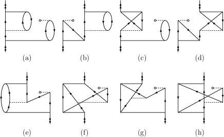
Figure 5: Goldstone HFS diagrams from ${S_{2}}^{\dagger}h_{\rm hfs}S_{3({\rm vs})}$, which contribute to $A_{({\rm vs})}^{1}$. In the first diagram (a) all the two body vertices, $S_{2}^{\dagger}$, $1/r_{12}$ and $S_{2}$ are of direct type. Remaining diagrams are combinations of exchange at different vertices.

VI HFS constants from $S_{2}$ perturbed triples

From the expression of HFS constant with RCC wave function in Eq. (35), the lowest order triples contributions are of the form

$$A_{3}=T_{1}^{\dagger}H_{\rm hfs}S_{3}+T_{2}^{\dagger}H_{\rm hfs}S_{3}+S_{2}^{\dagger}H_{\rm hfs}S_{3}.$$ (39)

The first term is, however, neglected in the present calculations. The reason is, the $T_{1}$ cluster amplitudes are small and have no significant contributions. For easy book keeping, contributions from the remaining two terms is bifurcated based on the nature of $H_{\rm hfs}$ matrix elements. Two of the possibilities, $\langle a|h_{\rm hfs}|p\rangle$ and $\langle v|h_{\rm hfs}|p\rangle$ are considered. There are 52 Goldstone HFS diagrams associated with these two matrix elements and the $S_{2}$ perturbed $S_{3}$. These are separated into groups and discussed in this section. The other forms, $\langle a|h_{\rm hfs}|a\rangle$ and $\langle p|h_{\rm hfs}|p\rangle$, enter through the structural radiation diagrams, which are negligibly small and are excluded from the present calculations.

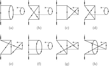
Figure 6: Goldstone HFS diagrams from ${S_{2}}^{\dagger}h_{\rm hfs}S_{3({\rm vs})}$, which contribute to $A_{({\rm vs})}^{2}$. In the first diagram (a) all the two body vertices, $S_{2}^{\dagger}$, $1/r_{12}$ and $S_{2}$ are of direct type. Remaining diagrams are combinations of exchange at different vertices.

VI.1 Contribution from $S_{2}^{\dagger}H_{\rm hfs}S_{3({\rm vs})}$

Consider the triples of the form $s_{vab({\rm vs})}^{pqr}$ defined in Eq. (12), for easy reference $S_{3({\rm vs})}$ define the general form of the triples in this group. The contraction $\mathchoice{\vbox{\hbox to0.0pt{\kern 0.0pt\kern 2.88078pt\hbox{\vrule width=0.50003pt,height=0.0pt,depth=2.15277pt\vrule width=13.26607pt,height=0.0pt,depth=0.50003pt\vrule width=0.50003pt,height=0.0pt,depth=2.15277pt}\hss}\vskip 2.15277pt\vskip 6.94444pt}}{\vbox{\hbox to0.0pt{\kern 0.0pt\kern 2.88078pt\hbox{\vrule width=0.50003pt,height=0.0pt,depth=2.15277pt\vrule width=13.26607pt,height=0.0pt,depth=0.50003pt\vrule width=0.50003pt,height=0.0pt,depth=2.15277pt}\hss}\vskip 2.15277pt\vskip 6.94444pt}}{\vbox{\hbox to0.0pt{\kern 0.0pt\kern 2.01656pt\hbox{\vrule width=0.50003pt,height=0.0pt,depth=2.15277pt\vrule width=9.38669pt,height=0.0pt,depth=0.50003pt\vrule width=0.50003pt,height=0.0pt,depth=2.15277pt}\hss}\vskip 2.15277pt\vskip 4.8611pt}}{\vbox{\hbox to0.0pt{\kern 0.0pt\kern 1.44038pt\hbox{\vrule width=0.50003pt,height=0.0pt,depth=2.15277pt\vrule width=8.1397pt,height=0.0pt,depth=0.50003pt\vrule width=0.50003pt,height=0.0pt,depth=2.15277pt}\hss}\vskip 2.15277pt\vskip 3.47221pt}}h_{\rm hfs}S_{3({\rm vs})}$ is diagrammatically realized through four unique topologies. First, take the case where $h_{\rm hfs}$ has a core-particle contraction with $S_{2}$ in $S_{3({\rm vs})}$ and contribution to $A$ is

$$A_{({\rm vs})}^{1} = \sum_{vab}\sum_{pqrs}\frac{1}{\epsilon_{vab}^{pqr}}\left({s_{va}^{pq}}^{*}h_{b}^{r}v_{sa}^{pq}s_{vb}^{sr}-{s_{va}^{pq}}^{*}h_{b}^{r}v_{sa}^{pq}s_{vb}^{rs}\right.$$ (40)

$$\left.-{s_{va}^{pq}}^{*}h_{b}^{r}v_{sa}^{qp}s_{vb}^{sr}+{s_{va}^{pq}}^{*}h_{b}^{r}v_{sa}^{qp}s_{vb}^{rs}\right),$$

where $h_{b}^{r}$ denotes the matrix element $\langle r|h_{\rm hfs}|b\rangle$. The many-body diagrams in Fig. 5a-d are the representation of the above terms. For compact notation, introduce the antisymmetrised representation of the residual Coulomb matrix element, $\tilde{v}_{ab}^{pq}=v_{ab}^{pq}-v_{ab}^{qp}=v_{ab}^{pq}-v_{ba}^{pq}$. Antisymmetrised representation of the $s_{va}^{pq}$ is defined in the same way. In a more compact form

$$A_{({\rm vs})}^{1}=\sum_{vab}\sum_{pqrs}\frac{1}{\epsilon_{vab}^{pqr}}{s_{va}^{pq}}^{*}h_{b}^{r}\tilde{v}_{sa}^{pq}\tilde{s}_{vb}^{sr}.$$ (41)

It must be noted that, the antisymmetrised form is employed for compact notations. Otherwise, all the calculations are in non symmetrised representations and is a better choice with diagrammatic analysis.

Second, the core and particle lines of $h_{\rm hfs}$ contracts with the residual Coulomb and $S_{2}$, respectively. Diagrams arising from the contractions are shown in Fig. 5e-h and contribution is

$$A_{({\rm vs})}^{2} = \sum_{vab}\sum_{pqrs}\frac{-1}{\epsilon_{vab}^{pqr}}\left({s_{bv}^{rq}}^{*}h_{a}^{p}v_{sa}^{rq}s_{bv}^{sp}-{s_{bv}^{rq}}^{*}h_{a}^{p}v_{sa}^{rq}s_{bv}^{ps}\right.$$ (42)

$$\left.-{s_{bv}^{rq}}^{*}h_{a}^{p}v_{sa}^{qr}s_{bv}^{sp}+{s_{bv}^{rq}}^{*}h_{a}^{p}v_{sa}^{qr}s_{bv}^{ps}\right).$$

In antisymmetrised representation

$$A_{({\rm vs})}^{2}=\sum_{vab}\sum_{pqrs}\frac{-1}{\epsilon_{vab}^{pqr}}{s_{bv}^{rq}}^{*}h_{a}^{p}\tilde{v}_{sa}^{rq}\tilde{s}_{bv}^{sp}.$$ (43)

The two cases discussed so far have double virtual orbital contraction of $S_{2}^{\dagger}$ with either residual Coulomb interaction or $S_{2}$. As a result no unique diagrams arise from the anti-symmetrization of the $S_{2}^{\dagger}$.

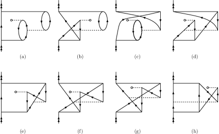
Figure 7: Goldstone HFS diagrams from ${S_{2}}^{\dagger}h_{\rm hfs}S_{3({\rm vs})}$, which contribute to $A_{({\rm vs})}^{3}$. In the first diagram (a) all the two body vertices, $S_{2}^{\dagger}$, $1/r_{12}$ and $S_{2}$ are of direct type. Remaining diagrams are combinations of exchange at different vertices.

Third, the core-virtual orbital lines of $h_{\rm hfs}$ contracts with the residual Coulomb interaction. Eight unique diagrams arise from the contractions and are shown in Fig.6. The contribution is

$$A_{({\rm vs})}^{3}=\sum_{vab}\sum_{pqrs}\frac{1}{\epsilon_{vab}^{pqr}}\left[{s_{va}^{pq}}^{*}h_{r}^{b}\tilde{v}_{sb}^{qr}\tilde{s}_{va}^{ps}-{s_{va}^{qp}}^{*}h_{r}^{b}\tilde{v}_{sb}^{qr}\tilde{s}_{va}^{ps}\right],$$ (44)

here, as in previous expressions the antisymmetrised $v$ and $S_{2}$ are used for compact notations. The antisymmetrised expression of $S_{2}^{\dagger}$ can be used to obtain the expression

$$A_{({\rm vs})}^{3}=\sum_{vab}\sum_{pqrs}\frac{1}{\epsilon_{vab}^{pqr}}\tilde{s}_{va}^{pq*}h_{r}^{b}\tilde{v}_{sb}^{qr}\tilde{s}_{va}^{ps}.$$ (45)

There is a prominent difference of the present case from the previous two, the exchange of $S_{2}^{\dagger}$ gives topologically unique diagrams.

Finaly, the core and virtual orbital line of $h_{\rm hfs}$ contract with the $S_{2}$ and residual Coulomb interaction, respectively. Diagrams from the contractions are shown in Fig. 6 and in antisymmetrised notations, the contribution is

$$A_{({\rm vs})}^{4}=\sum_{vab}\sum_{pqrs}\frac{1}{\epsilon_{vab}^{pqr}}\tilde{s}_{vb}^{pr*}h_{q}^{b}\tilde{v}_{sb}^{qr}\tilde{s}_{va}^{ps}.$$ (46)

In this case too, there are eight unique diagrams.

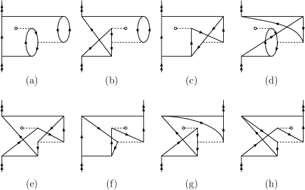
Figure 8: Goldstone HFS diagrams from ${S_{2}}^{\dagger}h_{\rm hfs}S_{3({\rm cs})}$, which contribute to $A_{({\rm cs})}^{1}$. In the first diagram (a) all the two body vertices, $S_{2}^{\dagger}$, $1/r_{12}$ and $S_{2}$ are of direct type. Remaining diagrams are combinations of exchange at different vertices.

VI.2 Contribution from $S_{2}^{\dagger}H_{\rm hfs}S_{3({\rm cs})}$

The triples of the $S_{3({\rm cs})}$ type have two virtual lines above the $S_{2}$ vertex and no core line. This limits the number of allowed contractions between $h_{\rm hfs}$ and $S_{2}$. So, there are only two unique topologies of the contraction $\mathchoice{\vbox{\hbox to0.0pt{\kern 0.0pt\kern 2.88078pt\hbox{\vrule width=0.50003pt,height=0.0pt,depth=2.15277pt\vrule width=13.26607pt,height=0.0pt,depth=0.50003pt\vrule width=0.50003pt,height=0.0pt,depth=2.15277pt}\hss}\vskip 2.15277pt\vskip 6.94444pt}}{\vbox{\hbox to0.0pt{\kern 0.0pt\kern 2.88078pt\hbox{\vrule width=0.50003pt,height=0.0pt,depth=2.15277pt\vrule width=13.26607pt,height=0.0pt,depth=0.50003pt\vrule width=0.50003pt,height=0.0pt,depth=2.15277pt}\hss}\vskip 2.15277pt\vskip 6.94444pt}}{\vbox{\hbox to0.0pt{\kern 0.0pt\kern 2.01656pt\hbox{\vrule width=0.50003pt,height=0.0pt,depth=2.15277pt\vrule width=9.38669pt,height=0.0pt,depth=0.50003pt\vrule width=0.50003pt,height=0.0pt,depth=2.15277pt}\hss}\vskip 2.15277pt\vskip 4.8611pt}}{\vbox{\hbox to0.0pt{\kern 0.0pt\kern 1.44038pt\hbox{\vrule width=0.50003pt,height=0.0pt,depth=2.15277pt\vrule width=8.1397pt,height=0.0pt,depth=0.50003pt\vrule width=0.50003pt,height=0.0pt,depth=2.15277pt}\hss}\vskip 2.15277pt\vskip 3.47221pt}}h_{\rm hfs}S_{3({\rm cs})}$. First, the core and virtual orbitals of $h_{\rm hfs}$ contract wit the residual Coulomb interaction and $S_{2}$, respectively. Diagrams arising from the contractions are shown in Fig. 8 and contribution in antisymmetrised notation is

$$A_{({\rm cs})}^{1}=\sum_{vab}\sum_{pqrs}\frac{-1}{\epsilon_{vab}^{pqr}}\tilde{s}_{vb}^{pr*}h_{q}^{a}\tilde{v}_{ab}^{cr}\tilde{s}_{vc}^{pq}.$$ (47)

And second, the $h_{\rm hfs}$ contracts with the orbital lines of residual Coulomb interactions. There are four diagrams and are shown in Fig. 9. The contribution is

$$A_{({\rm cs})}^{2}=\sum_{vab}\sum_{pqrs}\frac{-1}{\epsilon_{vab}^{pqr}}s_{va}^{pq*}h_{r}^{b}\tilde{v}_{ab}^{cr}\tilde{s}_{vc}^{pq}.$$ (48)

Note, the exchange at the $S_{2}^{\dagger}$, like in $A_{({\rm vs})}^{1}$ and $A_{({\rm vs})}^{2}$, does not generate topologically unique diagrams.

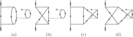
Figure 9: Goldstone HFS diagrams from ${S_{2}}^{\dagger}h_{\rm hfs}S_{3({\rm cs})}$, which contribute to $A_{({\rm cs})}^{2}$. In the first diagram (a) all the two body vertices, $S_{2}^{\dagger}$, $1/r_{12}$ and $S_{2}$ are of direct type. Remaining diagrams are combinations of exchange at different vertices.

VI.3 Contribution from $T_{2}^{\dagger}H_{\rm hfs}S_{3}$

There is a key topological difference between the $T_{2}^{\dagger}H_{\rm hfs}S_{3}$ and $S_{2}^{\dagger}H_{\rm hfs}S_{3}$ diagrams. This arises from the number of lines above vertex of the cluster operators $S_{2}$ and $T_{2}$. The former has three, where as the later has four and more operators to contract. Consequently, fewer diagrams arise from $T_{2}^{\dagger}H_{\rm hfs}S_{3}$ and these, like earlier, are identified based on the topology of contractions. Contributions from this term, like in $S_{2}^{\dagger}H_{\rm hfs}S_{3}$, is separable into $T_{2}^{\dagger}H_{\rm hfs}S_{3({\rm vs})}$ and $T_{2}^{\dagger}H_{\rm hfs}S_{3({\rm cs})}$. Consider the first term, there are two groups of diagrams. In the first group, ${T_{2}}^{\dagger}$ contracts with the a pair of core and virtual lines with $S_{2}$ and $v$. Eight distinct diagrams, shown in Fig. 10, arise from this contraction and contribution is

$$A_{({\rm vs})}^{5}=\sum_{vab}\sum_{pqrs}\frac{1}{\epsilon_{vab}^{pqr}}\tilde{t}_{ab}^{qr*}h_{p}^{v}\tilde{v}_{sb}^{pr}\tilde{s}_{va}^{sq}.$$ (49)

Here, we have given the antisymmetrised expression. The individual terms may be written in explicit forms line in Eq. (44).

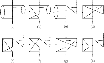
Figure 10: Goldstone HFS diagrams from ${S_{2}}^{\dagger}h_{\rm hfs}S_{3({\rm vs})}$, which contribute to $A_{({\rm vs})}^{5}$. In the first diagram (a) all the two body vertices, $S_{2}^{\dagger}$, $1/r_{12}$ and $S_{2}$ are of direct type. Remaining diagrams are combinations of exchange at different vertices.

The second group of diagrams arise from the contraction of ${T_{2}}^{\dagger}$ with two virtual and one core orbital lines of $v$, and one core orbital line of $S_{2}$. Four diagrams arise from this term and these are given in Fig. 11. The contribution in antisymmetrised form is

$$A_{({\rm vs})}^{6}=\sum_{vab}\sum_{pqrs}\frac{1}{\epsilon_{vab}^{pqr}}\tilde{t}_{ab}^{sr*}h_{p}^{v}v_{qb}^{sr}\tilde{s}_{va}^{pq}.$$ (50)

Note that ${T_{2}}^{\dagger}$ and $S_{2}$ are antisymmetrised in the above equation. Where as, $v$ and $S_{2}$ are antisymmetrised in the previous groups consisting of four diagrams. These two antisymmetrizations are equivalent and give the same set of diagrams. The term $A_{({\rm vs})}^{6}$ completes the possible forms of HFS diagrams arising from the $S_{3({\rm vs})}$ type of valence triples. Collecting all the terms, the net contribution is

$$A_{({\rm vs})}=\sum_{i=1}^{6}A_{({\rm vs})}^{i}.$$ (51)

To summarize, $A_{({\rm vs})}$ constitute 36 many-body Goldstone diagrams grouped into six groups. Each group is defined based on the contraction topology and form of $h_{\rm hfs}$.

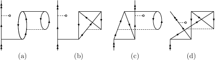
Figure 11: Goldstone HFS diagrams from ${S_{2}}^{\dagger}h_{\rm hfs}S_{3({\rm vs})}$, which contribute to $A_{({\rm vs})}^{6}$. In the first diagram (a) all the two body vertices, $S_{2}^{\dagger}$, $1/r_{12}$ and $S_{2}$ are of direct type. Remaining diagrams are combinations of exchange at different vertices.

From $T_{2}^{\dagger}H_{\rm hfs}S_{3({\rm cs})}$ there are two groups of diagrams. The first group has four diagrams and these are shown in Fig. 12a-d. The contribution is

$$A_{({\rm cs})}^{3}=\sum_{vabc}\sum_{pqr}\frac{1}{\epsilon_{vab}^{pqr}}\tilde{t}_{ab}^{qr*}h_{p}^{v}v_{ab}^{cr}\tilde{s}_{vc}^{pq}.$$ (52)

The second group has two diagrams and these are shown in Fig. 12e-f. The contribution is

$$A_{({\rm cs})}^{4}=\sum_{vabc}\sum_{pqr}\frac{-1}{\epsilon_{vab}^{pqr}}t_{ab}^{qp*}h_{r}^{v}v_{ab}^{dr}\tilde{s}_{dv}^{pq}.$$ (53)

Collecting all the groups, the net contribution from the $S_{3({\rm cs})}$ type of triples is

$$A_{({\rm cs})}=\sum_{i=1}^{4}A_{({\rm cs})}^{i}.$$ (54)

Totally there are 18 Goldstone diagrams in $A_{({\rm cs})}$. Collecting all the diagrams from the $S_{2}$ perturbed triples, we define

$$A_{({\rm s})}=A_{({\rm vs})}+A_{({\rm cs})}.$$ (55)

There are in 54 many-body diagrams and these are separable into ten groups. This completes, excluding the structural radiation diagrams, the diagrammatic analysis of the $S_{2}$ perturbed triple correction to the magnetic hyperfine constant.

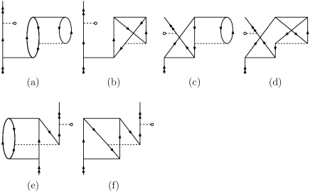
Figure 12: Goldstone HFS diagrams from ${S_{2}}^{\dagger}h_{\rm hfs}S_{3({\rm cs})}$, which contribute to $A_{({\rm cs})}^{3}$. In the first diagram (a) all the two body vertices, $S_{2}^{\dagger}$, $1/r_{12}$ and $S_{2}$ are of direct type. Remaining diagrams are combinations of exchange at different vertices.

VII HFS constants from $T_{2}$ perturbed triples

The contributions from the $T_{2}$ perturbed triples, like in $S_{2}$ perturbed triples, is separated into two categories: perturbation to the core orbital and virtual orbital. Contribution from these are defined as $A_{({\rm ct})}$ and $A_{({\rm vt})}$. Similar to $A_{(\rm s)}$, diagrams from each of these are classified into groups. Diagrams from each of the groups with direct at all the two body vertices are given in Fig. 13. The diagrams of the $A_{({\rm ct})}$ are shown in Fig. 13(a-d) and (g-h). The expression is

$$A_{({\rm ct})} = \sum_{vabc}\sum_{pqr}\frac{-1}{\epsilon_{vab}^{pqr}}\Big{(}s_{av}^{qp*}h_{r}^{b}\tilde{v}_{vb}^{cr}\tilde{t}_{ac}^{qp}-s_{av}^{qr*}h_{p}^{b}\tilde{v}_{av}^{cp}\tilde{t}_{cb}^{qr}$$ (56)

$$+\tilde{s}_{vb}^{pq*}h_{r}^{b}\tilde{v}_{vb}^{pc}\tilde{t}_{cb}^{qr}+\tilde{s}_{vb}^{pr*}h_{q}^{a}\tilde{v}_{va}^{pc}\tilde{t}_{cb}^{qr}+\tilde{t}_{ab}^{qr*}h_{p}^{v}\tilde{v}_{vb}^{cr}\tilde{t}_{ac}^{qp}$$

$$+\tilde{t}_{ab}^{qr*}h_{p}^{v}\tilde{v}_{va}^{pc}t_{cb}^{qr}\Big{)}.$$

One immediate observation is, the structure and number of the terms in the above expression are similar to $A_{({\rm vs})}$. Key transformations are interchange of conversion of $S_{2}$ and $v$ operators to $v$ and $T_{2}$, respectively. The expression of the second category is

$$A_{({\rm vt})} = \sum_{vab}\sum_{pqrs}\frac{1}{\epsilon_{vab}^{pqr}}\Big{(}\tilde{s}_{vb}^{pr*}h_{q}^{a}\tilde{v}_{vs}^{pq}\tilde{t}_{ab}^{sr}+s_{va}^{pq*}h_{r}^{b}\tilde{v}_{vs}^{pq}\tilde{t}_{ab}^{sr}$$ (57)

$$+\tilde{t}_{ab}^{qr*}h_{p}^{v}\tilde{v}_{vs}^{pq}\tilde{t}_{ab}^{sr}-t_{ab}^{qp*}h_{r}^{v}\tilde{v}_{sv}^{qp}t_{ab}^{sr}\Big{)}.$$

Here, the terms are similar to $A_{({\rm cs})}$ and same transformations discussed in $A_{({\rm ct})}$ apply.

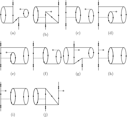
Figure 13: HFS diagrams from the $T_{2}$ perturbed $S_{3}$. Here, only the diagrams with direct interaction at all the interaction vertices are given.

Table 1: Basis set parameters $\alpha$ and $\beta$ used in the calculations.

Atom	Orbital	$\alpha$	$\beta$	Basis function
Rb	$s$	$0.00521$	$2.9500$	$33$
	$p$	$0.00655$	$2.9950$	$30$
	$d$	$0.00654$	$2.9720$	$28$
Sr+	$s$	$0.00825$	$2.9000$	$35$
	$p$	$0.00715$	$2.9450$	$32$
	$d$	$0.00730$	$2.9100$	$30$

VIII Results and discussions

VIII.1 Single particle states

The first step of our calculations, like in any atomic many-body calculations, is to solve the single particle eigenvalue equations with Dirac-Hartree-Fock potential. For this, we consider the nuclear potential $V_{N}(\mathbf{r})$ arising from the finite size Fermi density distribution

$$\rho_{\rm nuc}(r)=\frac{\rho_{0}}{1+e^{(r-c)/a}},$$ (58)

here, $a=t4\ln 3$. The parameter $c$ is the half-charge radius, that is $\rho_{\rm nuc}(c)=\rho_{0}/2$ and $t$ is the skin thickness. At the single particle level, the spin orbitals are of the form

$$\psi_{n\kappa m}(\mathbf{r})=\frac{1}{r}\left(\begin{array}[]{r}P_{n\kappa}(r)\chi_{\kappa m}(\hat{\mathbf{r}})\\ iQ_{n\kappa}(r)\chi_{-\kappa m}(\hat{\mathbf{r}})\end{array}\right),$$ (59)

where $P_{n\kappa}(r)$ and $Q_{n\kappa}(r)$ are the large and small component radial wave functions, $\kappa$ is the relativistic total angular momentum quantum number and $\chi_{\kappa m}(\hat{\mathbf{r}})$ are the spin or spherical harmonics. One representation of the radial components is to define these as linear combination of Gaussian like functions and are referred to as Gaussian type orbitals (GTOs). Then, the large and small components mohanty-89 ; chaudhuri-99 are

$$P_{n\kappa}(r)=\sum_{p}C^{L}_{\kappa p}g^{L}_{\kappa p}(r),$$

$$Q_{n\kappa}(r)=\sum_{p}C^{S}_{\kappa p}g^{S}_{\kappa p}(r).$$ (60)

The index $p$ varies over the number of the basis functions. For large component we choose

$$g^{L}_{\kappa p}(r)=C^{L}_{\kappa i}r^{n_{\kappa}}e^{-\alpha_{p}r^{2}},$$ (61)

here $n_{\kappa}$ is an integer. Similarly, the small component are derived from the large components using kinetic balance condition. The exponents in the above expression follow the general relation

$$\alpha_{p}=\alpha_{0}\beta^{p-1}.$$ (62)

The parameters $\alpha_{0}$ and $\beta$ are optimized for each of the ions to provide good description of the properties. In our case the optimization is to reproduce the numerical result of the total and orbital energies. The optimized parameters used in the calculations are listed in Table.1.

Table 2: Excitation energies calculated using RCC, compared with other theoretical results and experimental data. All values are in atomic units.

Atom	State	This work	Other works	Exp Refnist .
85Rb	$5s_{1/2}$	$0.0$	$0.0$	$0.0$
	$5p_{1/2}$	$0.05759$	$0.05718^{\rm a}$	$0.05731$
	$5p_{3/2}$	$0.05872$	$0.05826^{\rm a}$	$0.05840$
	$4d_{3/2}$	$0.08836$	$0.08822^{\rm a}$	$0.08819$
	$4d_{5/2}$	$0.08836$	$0.08820^{\rm a}$	$0.08819$
87Sr+	$5s_{1/2}$	$0.0$	$0.0$	$0.0$
	$5p_{1/2}$	$0.10841$	$0.11001^{\rm b}$	$0.10805$
	$5p_{3/2}$	$0.11221$	$0.11376^{\rm b}$	$0.11171$
	$4d_{3/2}$	$0.06611$	$0.06560^{\rm b}$	$0.06632$
	$4d_{5/2}$	$0.06724$	$0.06707^{\rm b}$	$0.06760$

^a Referencesafronova-11 ^b Referenceguet-91

For Rb and Sr⁺ we use $V^{N-1}$ and $V^{N-2}$ orbitals, respectively. These are the single particle eigenfunctions of the Rb⁺ and Sr²⁺ ions, respectively. The single particle basis sets have few bound states and rest are continuum. We optimize the basis such that: single particle energies of the core and valence orbitals are in good agreement with the numerical results. For this we use GRASP92 parpia-96 to generate the numerical results. It is to be noted that, the basis parameters in Table.1 are different from one give in our earlier work mani-10 . Between the two, the present is better optimized and of higher quality. The optimization is nontrivial as there are several parameters and single particle equations are solved self-consistently.

From Eq.(59) the reduced matrix element of the magnetic hyperfine operator between two spin orbitals , $v^{\prime}$ and $v$, is

$$\langle v^{\prime}|\!|t^{1}|\!|v\rangle = -(\kappa_{v}+\kappa_{v^{\prime}})\langle-\kappa_{v^{\prime}}|\!|C^{1}|\!|\kappa_{v}\rangle$$ (63)

$$\times\int^{\infty}_{0}\frac{dr}{r^{2}}(P_{n_{v^{\prime}}\kappa_{v^{\prime}}}Q_{n_{v}\kappa_{v}}+Q_{n_{v^{\prime}}\kappa_{v^{\prime}}}P_{n_{v}\kappa_{v}}).\;\;\;\;\;\;$$

A detailed derivation is given in Ref. johnson-07 .

VIII.2 Cluster amplitudes and normalization

As described in our earlier works mani-09 ; mani-10 ; mani-11 , the RCC equations are solved iteratively using the Jacobi method. To improve convergence we employ direct inversion in the iterated subspace (DIIS) pulay-80 . The cluster amplitudes are solved for each Hilbert space manifold of the total Fock space. At each step the Hilbert space is augmented with one electron. In short, the $T$ equations are solved first and these are used to generate the open shell cluster amplitudes $S$.

One important point is, the cluster equations are in terms of the reduced matrix elements. So the solutions are independent of magnetic quantum numbers and appropriate phase factors are required to define the cluster amplitudes in the cojugate manifold and these are

$$t_{a}^{p*} = (-1)^{j_{p}-j_{a}}t_{a}^{p},$$ (64)

$$t_{ab}^{pq*} = (-1)^{j_{p}+j_{q}-j_{b}-j_{a}}t_{ab}^{pq}.$$ (65)

These relations apply in any calculation which involve $T^{\dagger}$ and $S^{\dagger}$. The coupled-cluster wave function is normalized and the normalization factor is

$${\cal N}=\langle\Psi_{v}|\Psi_{v}\rangle=\langle\Phi_{v}|e^{T^{\dagger}}\left(1+S^{\dagger}\right)\left(1+S\right)e^{T}|\Phi_{v}\rangle.$$ (66)

Here, $e^{T^{\dagger}}e^{T}$ is a non-terminating operator. For the present we consider the approximation

$${\cal N}\approx\langle\Phi_{v}|1+S^{\dagger}S+T^{\dagger}T|\Phi_{v}\rangle.$$ (67)

The higher order terms ${(T_{1}^{\dagger})}^{\alpha}{(T_{2}^{\dagger})}^{\beta}{(T_{1})}^{\gamma}{(T_{2})}^{\delta}$, such that $\alpha+\beta>1$, $\gamma+\delta>1$ and $\alpha+\beta-\gamma-\delta=0$, are neglected. We also neglect the mixed operator term $(T_{1}^{\dagger}S_{2}+\textrm{c.c.})$ and higher orders.

VIII.3 Excitation energies

To determine the quality of the basis set and parameters, we compute the attachment energies of the ground state ($S_{1/2}$) and the first excited $P_{1/2}$, $P_{3/2}$, $D_{3/2}$ and $D_{5/2}$ states are calculated. Then the ionization potential (IP), the energy required to remove the valence electron, is the negative of the attachement energy $-E^{\rm att}$. To calculate the excitation energy (EE) of the state $|\Psi_{v}\rangle$, consider $E^{\rm att}_{g}$ and $E^{\rm att}_{v}$ as the attachment energies of the ground state and excited state. Then difference $E^{\rm att}_{v}-E^{\rm att}_{g}$ is the EE, it can as well be defined in terms of IPs.

Table 3: Magnetic dipole hyperfine structure constants for ⁸⁵Rb and ⁸⁷Sr⁺. The values given are in the unit of MHz.

Atom	State	This work		Other works	Experiment
		CCSD	CCSD(T)
85Rb	$5s_{1/2}$	$1030.94$	$1030.60$	$1011.1^{\rm a}$	$1011.91(2)^{\rm b}$
	$5p_{1/2}$	$120.69$	$120.67$	$120.4^{\rm a}$	$120.72(25)^{\rm b}$
	$5p_{3/2}$	$24.48$	$24.63$	$24.5^{\rm a}$	$24.99(1)^{\rm c}$
	$4d_{3/2}$	$7.85$	$7.80$	$-$	$7.3(35)^{\rm d},7.329(35)^{\rm e}$
	$4d_{5/2}$	$-4.78$	$-4.77$	$-$	$-5.2(3)^{\rm d}$
87Sr+	$5s_{1/2}$	$-1014.20$	$-1013.86$	$-10003.18^{\rm f},-1000^{\rm g}$	$1000.5(1.0)^{\rm j}$
	$5p_{1/2}$	$-178.73$	$-178.67$	$-178.40^{\rm f},-177^{\rm g},-175^{\rm h}$	$-$
	$5p_{3/2}$	$-35.28$	$-35.48$	$-35.11^{\rm f},-35.3^{\rm g},-30^{\rm h}$	$-36.0^{\rm j}$
	$4d_{3/2}$	$-46.30$	$-46.21$	$-47.36^{\rm f},-46.7^{\rm g}$	$-$
	$4d_{5/2}$	$1.71$	$1.71$	$2.51^{\rm f},1.1^{\rm g},2.156^{\rm i}$	$2.17^{\rm k}$

^a Referencesafronova-99 , ^b Referencearimondo-77 , ^c Referencearimondo-75 , ^d Referencelam-80 , ^e Referencemoon-09 , ^f Referenceyu-04 , ^g Referencemartensson-02 ,

^h Referenceheully-85 , ⁱ Referencesahoo-07 , ^j Referencebuchinger-90 , ^k Referencebarwood-03 .

Table 4: The HFS contributions from different terms in RCC. All the values are in MHz.

Atom	State	RCC terms
		DF	$\tilde{H}_{\rm hfs}$-DF	$S^{\dagger}\tilde{H}_{\rm hfs}$	$S^{\dagger}_{2}\tilde{H}_{\rm hfs}S_{1}$	$S^{\dagger}_{1}\tilde{H}_{\rm hfs}S_{1}$	$S^{\dagger}_{2}\tilde{H}_{\rm hfs}S_{2}$	Other	Norm
				$+c.c$	$+c.c.$
85Rb	$5s_{1/2}$	$646.003$	$-12.115$	$375.719$	$19.822$	$23.564$	$20.498$	$-22.231$	$1.020$
	$5p_{1/2}$	$69.883$	$-0.762$	$47.411$	$2.762$	$2.751$	$1.630$	$-1.760$	$1.010$
	$5p_{3/2}$	$12.417$	$-0.054$	$10.919$	$0.804$	$0.450$	$0.479$	$-0.312$	$1.009$
	$4d_{3/2}$	$3.116$	$0.127$	$3.153$	$0.119$	$1.014$	$0.685$	$-0.068$	$1.039$
	$4d_{5/2}$	$1.328$	$0.087$	$-4.694$	$-2.550$	$0.420$	$0.472$	$-.028$	$1.038$
87Sr+	$5s_{1/2}$	$-735.629$	$8.044$	$-284.856$	$-9.987$	$-8.594$	$-15.624$	$16.907$	$1.015$
	$5p_{1/2}$	$-122.123$	$1.369$	$-56.502$	$-2.155$	$-1.862$	$-1.566$	$2.217$	$1.010$
	$5p_{3/2}$	$-21.449$	$0.191$	$-13.023$	$-0.582$	$-0.307$	$-0.869$	$0.412$	$1.010$
	$4d_{3/2}$	$-31.401$	$-0.803$	$-12.400$	$-0.594$	$-0.428$	$-2.020$	$0.283$	$1.023$
	$4d_{5/2}$	$-13.091$	$-0.428$	$16.306$	$1.051$	$-0.177$	$-2.018$	$0.116$	$1.023$

VIII.4 HFS constants

To compute the hyperfine constants from the CCSD wave functions, we use Eq.(35). The results are listed in Table.3, for comparison the results of other theoretical calculations and experimental data are also given. As defined in Eq.(35), the coupled-cluster expression of the hyperfine structure constants is separated into three groups. The dominant contribution from the first term $\tilde{H}_{\rm hfs}$, up to first order in $T^{\dagger}$ and $T$, is

$$\tilde{H}_{\rm hfs}\approx H_{\rm hfs}+2H_{\rm hfs}T_{1}+T_{1}^{\dagger}H_{\rm hfs}\left(T_{1}+2T_{2}\right)+T_{2}^{\dagger}H_{\rm hfs}T_{2}.$$ (68)

Here, the first term is the Dirac-Fock (DF), which has the largest contribution. The factor two in the second and fourth terms accounts for the complex conjugate terms. The third term, second order in $T_{1}$, has one diagram and negligibly small contribution. The diagrams arising from the last term are topologically are the structural radiation diagrams and have neglible contributions. Topologically, these are insertion of $H_{\rm hfs}$ to the normalization diagrams and contribution from these are labelled as $\tilde{H}_{\rm hfs}-{\rm DF}$. Detailed diagrammatic analysis are given in our previous work mani-10 . The last two terms in Eq.(35) are approximated as

$$S^{\dagger}\tilde{H}_{\rm hfs} \approx 2S^{\dagger}\left(H_{\rm hfs}e^{T}\right)_{1},$$ (69)

$$S^{\dagger}\tilde{H}_{\rm hfs}S \approx S_{1}^{\dagger}H_{\rm hfs}\left(S_{1}+2S_{2}\right)+S_{2}^{\dagger}H_{\rm hfs}S_{2}.$$ (70)

Like in $\tilde{H}_{\rm hfs}$, the factor of two is to account for the complex conjugate terms. Based on this grouping, the contributions are listed in Table.4. In the following we present a detailed comparison of our magnetic hyperfine constants results with the earlier ones. As discussed later, some of our results are the best match with experimental data.

VIII.5 HFS constants contribution from triples

The HFS constants after including the perturbed triples are listed in the Table. 3. There is negligible contribution for $S_{1/2}$ and $P_{1/2}$ states. These are 0.03% and 0.02% for Rb and, 0.03% and 0.03% for Sr⁺. However, for $P_{3/2}$, $D_{3/2}$, and $D_{5/2}$ contributions from triples are not small and could be important in high precision atomic theory calculation. And these are 0.6%, 0.6% and 0.2% for Rb, and 0.6%, 0.2% and 0.5% for Sr⁺. The observed pattern of perturbed triples contribution is different from ⁸⁷Rb reported in Ref. safronova-11 . This could be on account of two factors: difference in the nature of the single particle basis functions, and isotope specific effects. The later may not be the dominant cause as the electron wavefunctions have little variation for isotopes of small mass differences. For Sr⁺ on the other hand, there are no previous theoretical work on the effects of triple excitations. However, our results exhibits trends similar to previous work on Ca⁺ sahoo-09 , which reported the contributions from triples as 0.002%, 0.08%, 0.10%, 0.11% and 0.29% for $S_{1/2}$, $P_{1/2}$, $P_{3/2}$, $D_{3/2}$, and $D_{5/2}$ states, respectively.

Table 5: The term wise contribution of HFS constants from triples for Rb. All values listed are in atomic units.

RCC term	$5s_{1/2}$	$5p_{1/2}$	$5p_{3/2}$	$4d_{3/2}$	$4d_{5/2}$
$A_{({\rm vs})}^{1}$	$0.083$	$0.013$	$0.013$	$-0.003$	$-0.054$
$A_{({\rm vs})}^{2}$	$0.027$	$0.000$	$0.014$	$0.004$	$0.002$
$A_{({\rm vs})}^{3}$	$0.200$	$0.003$	$0.024$	$0.020$	$0.000$
$A_{({\rm vs})}^{4}$	$0.064$	$-0.002$	$0.012$	$0.000$	$-0.028$
$A_{({\rm vs})}^{5}$	$-0.236$	$-0.017$	$-0.010$	$-0.002$	$-0.002$
$A_{({\rm vs})}^{6}$	$-0.135$	$-0.014$	$-0.008$	$-0.005$	$-0.004$
$A_{({\rm vs})}$	$0.003$	$-0.017$	$0.045$	$0.014$	$-0.086$
$A_{({\rm cs})}^{1}$	$-0.141$	$-0.007$	$0.024$	$-0.018$	$0.058$
$A_{({\rm cs})}^{2}$	$0.012$	$0.007$	$0.000$	$0.001$	$0.015$
$A_{({\rm cs})}^{3}$	$0.216$	$0.018$	$0.010$	$0.007$	$0.005$
$A_{({\rm cs})}^{4}$	$-0.037$	$-0.002$	$-0.001$	$-0.001$	$-0.001$
$A_{({\rm cs})}$	$0.050$	$0.016$	$0.033$	$-0.011$	$0.077$
$A_{({\rm ct})}^{1}$	$-0.219$	$-0.006$	$-0.005$	$0.000$	$0.000$
$A_{({\rm ct})}^{2}$	$-0.007$	$-0.002$	$0.000$	$-0.005$	$-0.001$
$A_{({\rm ct})}^{3}$	$-0.005$	$0.000$	$-0.002$	$0.001$	$-0.003$
$A_{({\rm ct})}^{4}$	$-0.007$	$-0.002$	$-0.002$	$-0.002$	$-0.007$
$A_{({\rm ct})}^{5}$	$-0.149$	$-0.015$	$-0.007$	$-0.011$	$-0.007$
$A_{({\rm ct})}^{6}$	$1.966$	$0.195$	$0.113$	$0.035$	$0.030$
$A_{({\rm ct})}$	$1.579$	$0.170$	$0.097$	$0.018$	$0.012$
$A_{({\rm vt})}^{1}$	$-0.084$	$-0.006$	$0.002$	$-0.014$	$0.007$
$A_{({\rm vt})}^{2}$	$0.008$	$-0.001$	$-0.002$	$-0.003$	$0.014$
$A_{({\rm vt})}^{3}$	$-1.782$	$-0.178$	$-0.099$	$-0.028$	$-0.023$
$A_{({\rm vt})}^{4}$	$0.054$	$0.006$	$0.004$	$0.004$	$0.003$
$A_{({\rm vt})}$	$-1.804$	$-0.179$	$-0.095$	$-0.041$	$0.001$

VIII.5.1 Rb

In the Table. 5, we have listed the individual contributions from the different groups of triples HFS diagrams for Rb. In all the cases we notice large cancellations. For $S_{1/2}$ and $P_{1/2}$ states, the leading order (LO) and next to leading order (NLO) contribution arise from $A^{6}_{\rm ct}$ and $A^{3}_{\rm vt}$. Each of these terms contribute $\approx$ 0.2%. However, the two are of opposite signs and cancel each other. The other dominant contributing terms are $A^{5}_{\rm vs}$ and $A^{3}_{\rm cs}$ with contrbutions $\approx$ 0.02%. The two contributions are opposite in sign and like in LO and NLO, there are large cancellations.

For the state $P_{3/2}$, $A^{6}_{\rm ct}$ and $A^{3}_{\rm vt}$ are again the LO and NLO terms with contributions of $\approx$ 0.5% and $\approx$ 0.4%, respectively. The two contributions are of opposite sign and nearly cancel. Other dominant contributions arise from $A^{3}_{\rm vs}$ and $A^{1}_{\rm cs}$, each of the contributions are $\approx$ 0.1%. Unlike the cases considered and discussed so far, the two are of same phase. For $D_{3/2}$ too like in $S_{1/2}$, $P_{1/2}$ and $P_{3/2}$, $A^{6}_{\rm ct}$ and $A^{3}_{\rm vt}$ are the LO and NLO terms. Contributions from these terms are $\approx$ 0.4%, but opposite in sign. The other dominant contributions are from $A^{3}_{\rm vs}$ and $A^{1}_{\rm cs}$ and these are $\approx$ 0.3% and $\approx$ 0.2%, respectively. Like in LO and NLO these are of opposite sign and nearly cancel.

The state $D_{5/2}$ shows a different pattern of contributions. Unlike the states discussed so far, the dominant LO term is $A^{1}_{\rm cs}$ and the contribution is about 1.2%. The NLO term is $A^{1}_{\rm vs}$ and has a contribution of $\approx$1.1%. and is opposite to the LO term. The terms $A^{6}_{\rm ct}$ and $A^{3}_{\rm vt}$, which are the LO and NLO of $S_{1/2}$, $P_{1/2}$, $P_{3/2}$ and $D_{3/2}$, are the third and fourth dominant terms. Contributions from these terms are $\approx$ 0.6% and $\approx$ 0.5%, respectively.

Table 6: The term wise contribution of HFS constants from triples for Sr⁺. All values listed are in atomic units.

RCC term	$5s_{1/2}$	$5p_{1/2}$	$5p_{3/2}$	$4d_{3/2}$	$4d_{5/2}$
$A_{({\rm vs})}^{1}$	$-0.066$	$-0.016$	$-0.015$	$-0.011$	$0.098$
$A_{({\rm vs})}^{2}$	$-0.020$	$0.001$	$-0.020$	$-0.005$	$0.001$
$A_{({\rm vs})}^{3}$	$-0.129$	$0.001$	$-0.039$	$-0.046$	$0.024$
$A_{({\rm vs})}^{4}$	$-0.045$	$0.000$	$-0.015$	$-0.001$	$0.070$
$A_{({\rm vs})}^{5}$	$0.212$	$0.027$	$0.016$	$0.012$	$0.010$
$A_{({\rm vs})}^{6}$	$0.109$	$0.018$	$0.011$	$0.026$	$0.020$
$A_{({\rm vs})}$	$0.061$	$0.031$	$-0.062$	$-0.025$	$0.223$
$A_{({\rm cs})}^{1}$	$0.092$	$0.008$	$-0.028$	$0.036$	$-0.098$
$A_{({\rm cs})}^{2}$	$-0.010$	$-0.004$	$0.000$	$-0.010$	$-0.055$
$A_{({\rm cs})}^{3}$	$-0.157$	$-0.022$	$-0.012$	$-0.032$	$-0.024$
$A_{({\rm cs})}^{4}$	$0.028$	$0.003$	$0.003$	$0.006$	$0.004$
$A_{({\rm cs})}$	$-0.047$	$-0.015$	$-0.037$	$0.000$	$-0.173$
$A_{({\rm ct})}^{1}$	$0.158$	$0.007$	$0.008$	$0.000$	$0.000$
$A_{({\rm ct})}^{2}$	$0.006$	$0.004$	$0.002$	$0.016$	$0.002$
$A_{({\rm ct})}^{3}$	$0.003$	$0.000$	$0.004$	$-0.001$	$0.006$
$A_{({\rm ct})}^{4}$	$0.005$	$0.002$	$0.001$	$0.005$	$0.024$
$A_{({\rm ct})}^{5}$	$0.107$	$0.017$	$0.008$	$0.092$	$0.059$
$A_{({\rm ct})}^{6}$	$-1.935$	$-0.302$	$-0.172$	$-0.327$	$-0.266$
$A_{({\rm ct})}$	$-1.656$	$-0.272$	$-0.149$	$-0.215$	$-0.175$
$A_{({\rm vt})}^{1}$	$0.069$	$0.010$	$-0.003$	$0.038$	$-0.030$
$A_{({\rm vt})}^{2}$	$-0.003$	$0.001$	$0.002$	$0.010$	$-0.032$
$A_{({\rm vt})}^{3}$	$1.786$	$0.281$	$0.155$	$0.268$	$0.209$
$A_{({\rm vt})}^{4}$	$-0.041$	$-0.008$	$-0.004$	$-0.033$	$-0.025$
$A_{({\rm vt})}$	$1.811$	$0.284$	$0.150$	$0.283$	$0.122$

VIII.5.2 Sr⁺

The contributions from different RCC terms for Sr⁺ are as listed in the Table. 6. For the states $S_{1/2}$, $P_{1/2}$ and $P_{3/2}$, the LO and NLO have the same pattern as Rb is observed. The only difference is, signs are reversed. For example, in the case of $S_{1/2}$ of Rb, $A^{3}_{\rm cs}$ and $A^{6}_{\rm ct}$ are positive in sign, and $A^{5}_{\rm vs}$ and $A^{3}_{\rm vt}$ have negative sign. The pattern is opposite in the case of Sr⁺. The reason is trivial and is on account of the opposite sign of $\mu$, which for Rb and Sr⁺ are positive and negative, respectively.

For $D_{3/2}$ state, the LO and NLO contributions are large in comparison to the case of Rb. The LO and NLO terms are $A^{6}_{\rm ct}$ and $A^{3}_{\rm vt}$, respectively, and contributions are $\approx$ 0.7% and $\approx$ 0.6%. The other dominant contributions are from $A^{3}_{\rm vs}$ and $A^{1}_{\rm cs}$, and these are smaller than Rb.

The state $D_{5/2}$ show the largest LO and NLO contributions among all the states. These are 15.5% and 12.2% from the terms $A^{6}_{\rm ct}$ and $A^{3}_{\rm vt}$, respectively. However, the total contribution is 3.3% as they are of opposite signs. The other dominant contribution arise from $A^{1}_{\rm vs}$ and $A^{1}_{\rm cs}$. Contributions from each of these terms are 5.7% but are opposite in sign.

Table 7: Excitation energies calculated using RCC for different sets of basis functions. All values are in atomic units.

Atom	State	Set 1	Set 2	Set 3	Set 4	Set 5
85Rb	$5s_{1/2}$	$0.0$	$0.0$	$0.0$	$0.0$	$0.0$
	$5p_{1/2}$	$0.05756$	$0.05754$	$0.05758$	$0.05759$	$0.05759$
	$5p_{3/2}$	$0.05869$	$0.05867$	$0.05871$	$0.05872$	$0.05871$
	$4d_{3/2}$	$0.08854$	$0.08854$	$0.08834$	$0.08836$	$0.08836$
	$4d_{5/2}$	$0.08854$	$0.08853$	$0.08834$	$0.08836$	$0.08836$
87Sr+	$5s_{1/2}$	$0.0$	$0.0$	$0.0$	$0.0$	$0.0$
	$4d_{3/2}$	$0.06772$	$0.06767$	$0.06611$	$0.06611$	$0.06607$
	$4d_{5/2}$	$0.06882$	$0.06877$	$0.06724$	$0.06724$	$0.06720$
	$5p_{1/2}$	$0.10836$	$0.10837$	$0.10840$	$0.10841$	$0.10841$
	$5p_{3/2}$	$0.11217$	$0.11217$	$0.11220$	$0.11221$	$0.11221$

VIII.6 Uncertainty estimates

Atomic properties calculated from RCC theory, in general, have three important sources of uncertanties. These are: omission of higher-$l$ orbital basis states, truncation of the dressed HFS operator $\tilde{H}_{\rm hfs}$ and truncation of the coupled cluster operator $T$. The error arising from the third source–is truncation of the CC operator–is almost mitigated with the inclusion of perturbative triples. So, effectively, HFS results presented in the Table. 3 have uncertainties from the first two sources. In the following we analyze and estimate the upper bound on the uncertanties arising from each of these sources.

The results presented in Table. 3 are the converged results with the orbitals up to $h$ symmetry. To define the converged basis set, we do a series of calculations where we start with a minimal basis size of 112 orbitals consisting of (1-14)$s$, (2-14)$p$, (3-15)$d$, (4-16)$f$, and (5-14)$g$. Where we have used the non-relativistic notations for compact representations. The basis set is increased by adding two orbitals in each symmetry in the successive sets of calculations till the change in the excitation energies and HFS constants are below $10^{-4}$. The values from different orbital basis sets are given in Table. 7 and 8. The total number of orbitals in the converged results is 177, and symmetry wise it is (1-19)$s$, (2-19)$p$, (3-20)$d$, (4-21)$f$, (5-19)$g$ and (6-15)$h$. The single particle energies considered are $\approx 10^{5}$ Hartrees for $s$, $p$, $d$ and $f$ orbitals and, $\approx 10^{3}$ Hartree for $g$ and $h$.

To estimate the uncertanties from excluding higher symmetries, we include orbitals of $i$ symmetry and compute the HFS constants. For $S_{1/2}$, the largest contribution is in the case of Rb and is about 0.07%. However, for the states $P_{1/2}$ and $P_{3/2}$ it is Sr⁺ which has large contribution from the $i$ symmetry. These are 0.03% and 0.04% respectively for the states $P_{1/2}$ and $P_{3/2}$. Unlike the $S_{1/2}$, $P_{1/2}$ and $P_{3/2}$ states, the triples contributions for $D_{3/2}$ and $D_{5/2}$ are in general large. These are 1.2% for $D_{3/2}$ in the case of Rb and 7.0% for $D_{5/2}$ in the case of Sr⁺. In the present implementation of RCC theory, incorporating $j$ and higher symmetry basis states renders the basis set too large for computations. However, a leading-order analysis is possible with MBPT and we find the contribution from $j$ symmetry is negligible.

Table 8: The HFS constants calculated using RCC for different sets of basis functions. All values listed are in units of MHz.

Atom	State	Set 1	Set 2	Set 3	Set 4	Set 5
85Rb	$5s_{1/2}$	$1029.19$	$1027.78$	$1030.70$	$1031.00$	$1030.94$
	$5p_{1/2}$	$120.66$	$120.59$	$120.66$	$120.71$	$120.69$
	$5p_{3/2}$	$24.47$	$24.45$	$24.48$	$24.48$	$24.48$
	$4d_{3/2}$	$7.54$	$7.52$	$7.84$	$7.84$	$7.85$
	$4d_{5/2}$	$-4.78$	$-4.74$	$-4.79$	$-4.78$	$-4.78$
87Sr+	$5s_{1/2}$	$-1012.82$	$-1012.97$	$-1014.09$	$-1014.20$	$-1014.20$
	$5p_{1/2}$	$-178.61$	$-178.63$	$-178.67$	$-178.75$	$-178.73$
	$5p_{3/2}$	$-35.25$	$-35.25$	$-35.28$	$-35.28$	$-35.28$
	$4d_{3/2}$	$-45.90$	$-45.92$	$-46.21$	$-46.31$	$-46.30$
	$4d_{5/2}$	$2.085$	$2.07$	$1.73$	$1.72$	$1.71$

To estimate the uncertanties arising from the truncation of dressed properties operator, we resort to our previous work mani-10 . Where we proposed an iterative scheme to account for the higher order terms in the dressed properties operator $\tilde{H}_{\rm hfs}$. Using this scheme, we computed HFS constants contributions from the RCC terms which have loe of zero and one. These are the categories of diagrams which contribute most to the atomic properties using RCC. Contributions from the loe zero are 0.009%, 0.008%, 0.02%, 0.03% and 1.5%, respectively for $S_{1/2}$, $P_{1/2}$, $P_{3/2}$, $D_{3/2}$ and $D_{5/2}$ states of Sr⁺. From the loe one, however, these are large 0.09%, 0.24%, 0.35%, 0.22% and 12.40%. The loe two and higher are not considered as it involve higher-order terms in T which will naturally have smaller contributions.

In addition to the sources of errors discussed so far, the other sources of errors are the QED corrections. However, this cannot be considered as the source of error of the many-body method. It is rather the form of interaction considered in the calculations.

To put an upper bound on the uncertainty in the HFS results, we select and add the largest change from each of the sources. Which turn out approximately to be 0.2%, 0.3%, 0.4% and 1.5% for the states $S_{1/2}$, $P_{1/2}$, $P_{3/2}$ and $D_{3/2}$, respectively. For the state $D_{5/2}$, since there is large cancellations, a comprehensive analysis is necessary to arrive at a meaningful uncertainty estimate.

IX Conclusions

We derive and propose a general tensor representation of the triple cluster operator is symmetric and with proper phase the core and virtual orbital indices may be permuted. The permuation properties are derived from the rules of angular momentum diagrams. Although, we have discussed the triple cluster operator in the context of valence triples $S_{3}$, the same definition applies to core triples $T_{3}$. This may be explicitly demonstrated with a minor topological transformation of the cluster operator. Based on the generalized tensor representation of $S_{3}$, we derive the linearized RCC equation for CCSDT approximation.

We have analysed the contributions from the triple excitation cluster operators to the HFS constants in detail. For the analysis we identify two groups of diagrams depending on the nature of contractions to generate the triple cluster operator. In most of the cases the LO and NLO are identified as $A^{6}_{\rm ct}$ and $A^{3}_{\rm vt}$. These arise from the triples through the perturbation of $T_{2}$ cluster operators. From the results, for HFS constants computations with perturebed triple excitation cluster operators, it is sufficient to approximate

$$A=A^{1}_{\rm cs}+A^{3}_{\rm cs}+A^{6}_{\rm ct}+A^{3}_{\rm vs}+A^{5}_{\rm vs}+A^{3}_{\rm vt}.$$ (71)

Contributions from the remaining terms are negligible and can be excluded from the computations.

The total number of diagrams considered in the present calculations are 108. Number of diagrams, however, will decrease significantly with geniune valence triple cluster operators $S_{3}$ as the separation into core perturbed and virtual perturbed cluster is not applicable.

In conclusion, for calculations with the Gaussian type and $V^{N-1}$ potential orbital basis, the contributions from the triple excitation cluster operators is is at the most 0.6%.

- (1) F. Coester, Nucl. Phys. 7, 421 (1958).
- (2) F. Coester and H. Kümmel, Nucl. Phys. 17, 477 (1960).
- (3) R. J. Bartlett and M. Musial, Rev. Mod. Phys. 79, 291 (2007).
- (4) H. S. Nataraj, B. K. Sahoo, B. P. Das, and D. Mukherjee, Phys. Rev. Lett. 101, 033002 (2008).
- (5) R. Pal, M. S. Safronova, W. R. Johnson, A. Derevianko, and S. G. Porsev, Phys. Rev. A 75, 042515 (2007).
- (6) G. Hagen, T. Papenbrock, D. J. Dean, and M. Hjorth-Jensen, Phys. Rev. Lett. 101, 092502 (2008).
- (7) T. A. Isaev, A. N. Petrov, N. S. Mosyagin, A. V. Titov, E. Eliav, and U. Kaldor, Phys. Rev. A 69, 030501(R) (2004).
- (8) R. F. Bishop, P. H. Y. Li, D. J. J. Farnell, and C. E. Campbell, Phys. Rev. B 79, 174405 (2009).
- (9) K. V. P. Latha, D. Angom, B. P. Das, and D. Mukherjee, Phys. Rev. Lett. 103, 083001 (2009).
- (10) B. K. Sahoo, Phys. Rev. A 80, 012515 (2009)
- (11) C. Thierfelder and P. Schwerdtfeger, Phys. Rev. A 79, 032512 (2009).
- (12) B. K. Sahoo, B. P. Das, and D. Mukherjee, Phys. Rev. A 79, 052511 (2009).
- (13) L. W. Wansbeek, B. K. Sahoo, R. G. E. Timmermans, K. Jungmann, B. P. Das, and D. Mukherjee, Phys. Rev. A 78, 050501(R) (2008).
- (14) V. A. Dzuba, V. V. Flambaum, and J. S. M. Ginges, Phys. Rev. D 66, 076013 (2002).
- (15) C. S. Wood, et al. Science 275, 1759 (1997).
- (16) B. K. Sahoo, P. Mandal and M. Mukherjee, Phys. Rev. A 83 , 030502 (2011).
- (17) K. P. Geetha, A. D. Singh, B. P. Das, and C. S. Unnikrishnan, Phys. Rev. A 58, R16 (1998).
- (18) A. D. Singh and B. P. Das, J. Phys. B 32, 4905 (1999).
- (19) V. A. Dzuba, V. V. Flambaum, Phys. Rev. A 83, 052513 (2011).
- (20) V. A. Dzuba, V. V. Flambaum, Phys. Rev. A 83, 042514 (2011).
- (21) B. K. Mani and D. Angom, arXiv:1104.3473v1.
- (22) B. K. Mani and D. Angom, arXiv:1105.3447.
- (23) B. K. Mani, K. V. P. Latha, and D. Angom, Phys. Rev. A 80, 062505 (2009).
- (24) B. K. Mani and D. Angom, Phys. Rev. A 81, 042514 (2010).
- (25) B. K. Sahoo, Phys. Rev. A 80, 012515 (2009).
- (26) I. Lindgren and J. Morrison, Atomic Many-Body Theory, edited by G. Ecker, P. Lambropoulos, and H. Walther (Springer-Verlag, 1985).
- (27) S. G. Porsev and A. Derevianko, Phys. Rev. A 73, 012501 (2006).
- (28) W. R. Johnson, Atomic Structure Theory: Lectures on Atomic Physics (Springer Verlag, Berlin, 2007). Phys. Rev. A 59, 1187 (1999).
- (29) C. Schwartz, Phys. Rev. 97, 380 (1955).
- (30) A. K. Mohanty and E. Clementi, Chem. Phy. Lett., 157, 348 (1989).
- (31) R. K. Chaudhuri, P. K. Panda, and B. P. Das, Phys. Rev. A 59, 1187 (1999).
- (32) F. A. Parpia, C. Froese Fischer, and I. P. Grant, Comp. Phys. Comm. 94, 249 (1996).
- (33) NIST Atomic Spectroscopic Database, http://physics.nist.gov/PhysRefData.
- (34) M. S. Safronova and U. I. Safronova Phys. Rev. A 83, 052508 (2011).
- (35) C. Guet and W. R. Johnson, Phys. Rev. A 44, 1531 (1991).
- (36) B. K. Mani and D. Angom, Phys. Rev. A 83, 012501 (2011).
- (37) P. Pulay, Chem. Phys. Lett. 73, 393 (1980).
- (38) M. S. Safronova, W. R. Johnson and A. Derevianko, Phys. Rev. A 60, 4476 (1999).
- (39) E. Arimondo, M. Inguscio and P. Violino Rev. Mod. Phys. 49, 31 (1977).
- (40) E. Arimondo and M. Krainska-Miszczak, J. Phys. B: At. Mol. Phys. 8, 1613 (1975).
- (41) L. K. Lam, R. Gupta and W. Happer, Phys. Rev. A 21, 1225 (1980).
- (42) H. S. Moon, W-k. Lee and H. S. Suh Phys. Rev. A 79, 062503 (2009).
- (43) K.-z. Yu, L.-j. Wu, B.-c. Gou, and T.-y. Shi, Phys. Rev. A 70, 012506 (2004).
- (44) A-M. Martensson-Pendrill, J. Phys. B 35, 917 (2002).
- (45) J-L. Heully and A-M. Martensson-Pendrill, Phys. Scr. 31, 169 (1985).
- (46) B. K. Sahoo, C. Sur, T. Beier, B. P. Das, R. K. Chaudhuri, and D. Mukherjee, Phys. Rev. A 75, 042504 (2007).
- (47) F. Buchinger et al., Phys. Rev. C 41, 2883 (1990).
- (48) G. P. Barwood, K. Gao, P. Gill, G. Huang, and H. A. Klein, Phys. Rev. A 67, 013402 (2003).