Pricing stocks with yardsticks and sentiments

Abstract

Human decision making by professionals trading daily in the stock market can be a daunting task. It includes decisions on whether to keep on investing or to exit a market subject to huge price swings, and how to price in news or rumors attributed to a specific stock. The question then arises how professional traders, who specialize in daily buying and selling large amounts of a given stock, know how to properly price a given stock on a given day? Here we introduce the idea that people use heuristics, or “rules of thumb”, in terms of “yard sticks” from the performance of the other stocks in a stock index. The under-/over-performance with respect to such a yard stick then signifies a general negative/positive sentiment of the market participants towards a given stock. Using empirical data of the Dow Jones Industrial Average, stocks are shown to have daily performances with a clear tendency to cluster around the measures introduced by the yard sticks. We illustrate how sentiments, most likely due to insider information, can influence the performance of a given stock over period of months, and in one case years.

I Introduction

One of the founders of Behavioral Finance, D. KahnemanShefrin , once pointed out the close resemblance in the media coverage of financial markets to a stereotypical individual. As he mentioned, the media often describe financial markets with attributes like “… thoughts, beliefs, moods and sometimes stormy emotions. The main characteristic of the market is extreme nervousness. It is full of hope one moment and full of anxiety the next day …”. One way to get a first quantification of the sentiment of the market is to probe the sentiments of its investors. Studying sentiments of consumers/investors and its impact on markets has become an increasingly important topic. A various number of sentiment indices of investors/consumers already exists, some of which have now been recorded in a time span over some few decades. The Michigan Consumer Sentiment index, published monthly by the University of Michigan and Thomson Reuteurs, is probably the one which has the largest direct impact on markets when published. The natural question then arises as to whether it is possible to predict market movements based on the sentiments of consumers/investors?

Fisher and Statman FS made a study of tactical asset allocation from data of the sentiment of a heterogeneous group (large,medium,small) of investors. The main idea in FS was to look for indicators for future stock returns based on the diversity of sentiments. The study found the sentiments of different groups do not move in lockstep, and that sentiments for the groups of large and small investors, could be used as contrary indicators for future S&P 500 returns. Similar results were found by Baker and Wurgler who showed that when beginning-of-period proxies for sentiments are low, subsequent returns are relatively high for securities whose valuations are highly subjective and difficult to arbitrageBW However other papers are reporting on feedback loops between sentiment and market performance: past market returns determine investors sentiment who often expect a continuation of short term returnsBC . Recent researchTetlock on investors sentiment expressed in the media (as measured from the daily content of a Wall Street Journal column) seem to point in this direction with high media pessimism predicting downward pressure on market prices. Such results are in line with theoretical models of noise and liquidity tradersDSSW1 ; DSSW2 . Other studiesAF claim very little predictability on stock returns using computational linguistics to extract sentiments on 1.5 million internet message boards posted on Yahoo! Finance and Raging Bull. However in that study it was shown that disagreement induces trading and message posting activity was shown to correlate with volatility of the market.

Common to all the aforementioned studies is the aim to predict global market movements from sentiments either obtained in surveys or internet message boards. In the following we instead propose to obtain a sentiment related pricing of a given asset by expressing the relative sentiment of a given stock to the market. This is similar to the principle of the Capital Asset Price ModelCAPM (CAPM) which relates the price of a given asset to that of the price of the market, instead of trying to give absolute the price level of the asset/market. Put differently: we will in the following introduce a method that does not estimate the impact of a given “absolute” level of sentiment can have on the market, but instead introduce a sentiment of an asset relative to the sentiment of the general market whatever the absolute (positive/negative) sentiment of the general market. As will be illustrated this gives rise to a pricing formula for a given stock relative to the general market, much like the CAPM, but now with the relative sentiment of the stock to the market included in the pricing.

II Theory

We will in the following consider how traders find the appropriate price level of a given stock on a daily basis. One could for example have in mind traders that specialize on a given stock, who follow actively its price movements, maybe to consider opportune moments to either buy some amounts or instead sell as a part of a larger order. The question is what influences the decision making for traders when to enter and when to exit the market? According to the standard economic view only expectations about future earning/dividends and future interest rate levels should matter in the pricing of a given stock. Looking at the often very big price swings during earnings or interest rate announcements, this part clearly seem to play a major role at least at some specific instances of time. But what about other moments when there is no news which can be said to be relevant for future earnings/interest rates? The fluctuations seen in daily stock prices simply can not be explained by new information related to these two factors, nor can risk aversion, so why do stock prices fluctuate so much and how do traders navigate the often rough seas of fluctuations?

Here we will take a heuristics point of view, and argue that traders need some rule of thumb, or as we prefer to refer to it, “yardsticks”, in order to know how to position themselves. A first rough estimate for a trader would obviously be the returns of other stocks in a given stock index. Let us denote $s_{i}(t)$ the daily (nominal) return of stock $i$ belonging to the given index at time $t$, and $R_{-i}(t)$ the return of the remaining $N-1$ stocks in the index at time $t$. We emphasis to exclude the contribution of stock $i$ in $R_{-i}$ in order to avoid any self-impact which would amount to assuming that “the price of a stock rises because it rises”. Using the averaged return of the other stocks as a first crude yardstick one would then have that traders of stock $i$ would price the stock according to

$$s_{i}(t)\simeq R_{-i}(t)\equiv{1\over(N-1)}\sum_{j\neq i}s_{j}(t)$$ (1)

A powerful tool to check an equation, often used in Physics, is to use dimensional analysis and ensure that the quantities of both sides have the same dimensions. By the same token, an expression should be independent of the unit used. Since eq. (1) expresses a relationship between returns, i.e. a quantity that expresses increments in percentages, it is already dimensionless. However we argue that there is a mental relevant “unit” in play, which is the size of a typical daily fluctuation of a given stockJVA . Such a mental “unit of fluctuation” is created by the memory of traders who follow closely past performance of a given stock. Since the capacity of human working memory is quite small, investors are not able to analyze all available data. This causes individuals to simplify the world around themBEA . Investors need to choose consciously or unconsciously data that seem to be the most informative. While doing it (whatever the mode they are in) investors are exposed to the recency effect according to which they will remember recent prices better than earlier onesMC . The most recent prices are stored in short-term memory and therefore are easier to be retrieved than earlier ones that are stored in long-term memory. Hereby, the last volatility of the stock becomes a “unit of fluctuations” which investors refer to while anticipating future price changes. This “unit” which enters their attention field, influences their ability to estimate probabilities in accordance with the rule that events that are easier to be retrieved from the memory seem to be more likely to people than they really areTK . Dividing (1) on each side by the size of a typical fluctuation would therefore be one way to ensure independence of such units. Taking the standard deviation as measure of a typical fluctuation, the renormalized (1) takes the form:

$${s_{i}(t)\over\sigma(s_{i})}={R_{-i}(t)\over\sigma(R_{-i})}.$$ (2)

Here the standard deviation $\sigma(X)$ of the variable $X$ is defined over a given window size $T$ from the variance $\sigma^{2}={\rm Var}\equiv E_{T}(X^{2})-E_{T}^{2}(X)$, with $E$ denoting the expectation value.

As we will show in a moment, for most stocks over daily time periods of time (2) turns out to be a good approximation. There are however strong and persistent deviations. Actually we will in the following define stocks for which (2) holds on average, as “neutral” with respect to the sentiment of the traders. Similarly we use the relation as a measure of how biased (positive or negative) a sentiment traders have on the given stock. More precisely the sentiment of a given stock $i,\alpha_{i}$, is defined as:

$$\alpha_{i}(t)={s_{i}(t)\over\sigma(s_{i})}-{R_{-i}(t)\over\sigma(R_{-i})}.$$ (3)

We emphasize that the sentiment is defined with respect to the other stocks in the index, which serves as the neutral reference. The ratio of a stock’s (excess) return to its standard deviation, tells something about its performance, or reward-to-variability ratio, also called the Sharpe ratio in FinanceSharpe . Therefore (3) attributes a positive (respective negative) bias/sentiment to a stock, $\alpha_{i}>0$ (respective $\alpha_{i}<0$), when the Sharpe ratio of the stock exceeds (respective underperforms) the Sharpe ratio of the sum of the other stocks in the indexnote2 .

Rewriting (3) the pricing of stock $i$ can now be given in terms of a renormalized performance of the other stocks in the index as well as an eventual bias:

$$s_{i}(t)=\sigma(s_{i})\alpha_{i}(t)+{\sigma(s_{i})\over\sigma(R_{-i})}R_{-i}(t)$$ (4)

As a first check of (4) we take the expectation value of (4) by averaging over all stocks that an index is composed of, and average over time (daily returns). A priori, over long periods of time one would expect to find as many positive biased as negative biased stocks in an index composed of many stocks. That this is indeed the case will be shown empirically. Using this assumption the term with $\alpha_{i}$ disappears due to symmetry. One gets:

$$E(s_{i})={E(R_{-i})\over\sigma(R_{-i})}\sigma(s_{i})$$ (5)

(5) is very similar in structure to the famous Capital Asset Pricing Model in Finance (CAPM)note1 :

$${E(s_{i})-R_{f}\over\beta_{i}} = E(R)-R_{f};\beta_{i}={{\rm Cov}(s_{i},R)\over\sigma^{2}(R)}$$ (6)

$R_{f}$ in (6) is the risk free return which, since we consider daily returns, will be taken equal 0 in the following:

$$E(s_{i}) = {{\rm Cov}(s_{i},R)\over\sigma^{2}(R)}E(R).$$ (7)

Apart from the exclusion of the stock itself in the expression $R_{-i}$, the main difference between the CAPM in the form (7) and our hypothesis (5) is that we stress the use of standard deviations in the pricing formula instead of the covariance between the stock return and the index return on the right side of (7). Furthermore we argue that the covariance between a given stock and the index is not a very stable measure over time, whereas this is the case for the variance of a given stock. One reason for instability of the covariance could for example be created by sudden “shocks” in terms of specific bad or good news for a given company. After such a “shock” we postulate that the covariance between the stock and the index changes, whereas the stocks variance remain the same but with a change in relative performance as expressed through (3). (5) is reminiscent of the so-called capital allocation line in Finance which expresses the return of a portfolio composed of a certain percentage of the market portfolio and the remaining invested in a risk free asset. The capital allocation line however only expresses the return of this specific portfolio, whereas our expression is supposed to hold for each individual asset.

III Results

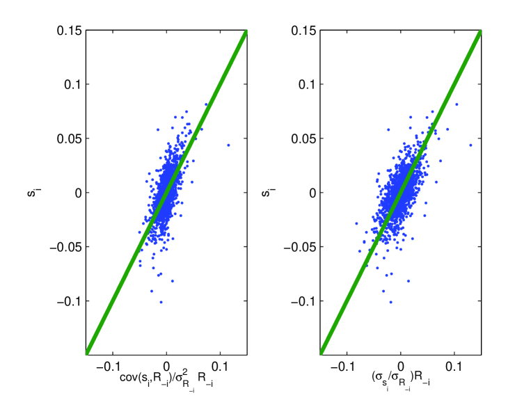
Figure 1: The plot to the left shows the CAPM hypothesis (7) using the daily returns of the Dow Jones Industrial index over the period 03/01/2000 to 20/06/2008. Plot to the right illustrates instead (5) using same data set. Each point correspond to a daily return $s_{i}$ of a given stock $i$.

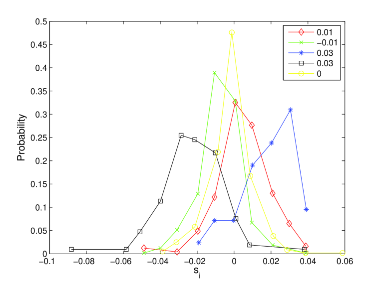
Figure 2: Probability distribution function of $s_{i}$ conditioned on 5 different values of $x\equiv{R_{-i}\over\sigma(R_{-i})}\sigma(s_{-i})$ This figure is inset to figure 1.

The data points in figure 1 show the CAPM hypothesis (7), and our hypothesis (5) respectively, using daily returns of the 30 stocks of the Dow Jones Industrial Average over almost a decade of datanote3 . A perfect fit of the data to the two equations would in both cases lie on the green diagonal. The data for CAPM appear tilted with respect to the diagonal, whereas the data concerning our hypothesis appear to be symmetrically distributed around the diagonal, which is what one should expect if the data on average followed (5). Figure 1b therefore gives some first evidence for the support of (5). This impression is strengthened when one takes a closer look at the cloud of data points in figure 1b, and consider the probability that the return of stock $i$ takes the value $s_{i}$, conditioned on a given fixed value of $x\equiv{R_{-i}\over\sigma(R_{-i})}\sigma(s_{i})$. Figure 2 shows the probability distribution function of $s_{i}$ conditioned on five different values of the variable $x$. From the hypothesis (4)-(5) one would expect the most likely value of the stock return $s_{i}$ to occur for the given fixed value of $x$. This is indeed seen to be the case with all five distributions peaking, if not actually at then close to $x$, giving further evidence to the assumption (5).

The sentiment $\alpha$ in (3) was introduced as a behavioral trait, and as such we would expect to see its effect on a long term time scale say at least of the order weeks or months. Figure 3 shows the cumulative sentiment for three different stocks, Citi Bank, and Caterpilar in the time period (03/01/2000 to 20/06/2008) and Cisco in the time period (01/06/2009 to 02/06/2011). The plots to the left shows in green the return of the Dow Jones and in blue the given stock over the given time period. The case of the Citi Bank stock is particular striking with a constant negative sentiment seen by the continuous decline in the cumulative sentiment curve of figure 3, corresponding to a constant sub-performance over two years. It should be noted that the data was chosen in order to have both a declining general market, which happens over the first half of the time period shown, as well as an increasing market which happens over the rest of the time period chosen. It is remarkable that the negative sentiment of the Citi Bank stocks stays constant independent of whether the general trend is bullish or bearish. Similarly it should be noted that the general sentiment of Caterpilar had a neutral value in the declining market, but then developed a distinguishable negative sentiment over the last three or four months of the time series where the general market is bullish. The price history for Cisco Systems tells a similar story. The only difference here is the two big jumps happening after 350 and 400 days respectively. These two particular events took place on the 11/11/2010 and on the 10/2/2011. On the 11/11/2010 the price dropped because of a bad report for the third quarter earnings. This gave rise to a loss of confidence by investors who were expecting a sign of recovery after a couple of hard months. On the 10/2/2011 Cisco Systems announced a drop in their earnings (down 18%) together with a downward revision (-7 %) of sales for their core product. It is worth noticing that the decline of the cumulative sentiment took place before the two events: prior to 11/11/2010 there was a long slow descent of the cumulative sentiment (meaning a constant negative sentiment) and after the 11/11/2010 the descent continued. This could be taken as evidence that some investors with insider knowledge were aware of the problems of the company, which was revealed only to the public on the two aforementioned days.

Figure 4 shows the probability distribution function of the sentiment variable obtained by sampling the sentiment variable $\alpha$ defined in (3), using the daily return of all stocks of the Dow Jones Industrial Average in the period 03/01/2000-20/06/2008. As can be seen from the inset of figure 4 the distribution appears to follow an exponential distribution for both positive and negative sentiments. One notes that the empirical distribution appears to be symmetric with respect to the sign of the sentiment - something which was implicitely assumed in deriving (5) from (4).

IV Discussion

The psychological experiments initiated by Kahneman and TverskyTK more than three decades ago showed that not only do people not behave rationally, but what is even more important: people do not behave randomly - people are suceptible to common judgment errors. Therefore research on sentiments is important because neither the efficient market hypothesis nor the noise trader theory explains systematic deviations of asset prices from fundamental values. So far sentiments in financial markets have been explained as either due to human overreaction or underreaction. For example Barberis et al.Barberis used psychological reasoning in explaning market deviations: overreaction with representativeness heuristics and underreaction with conservatism.

In this paper we have instead pointed out the importance of a relative sentiment measure of a given stock to its peers. The idea is that people use heuristics, or “rules of thumb”, in terms of “yard sticks” from the performance of the other stocks in a stock index. The under-/over-performance with respect to a yard stick then signifies a general negative/positive sentiment of the market participants towards a given stock. The bias created in such cases does not necessarily have a psychological origin but could be due to insider information. Insiders having superior information about the state of a company reduce/increase their stock holding gradually causing a persisting bias over time. The introduction of a measure for the relative sentiment of a stock has allowed us to come up with a pricing formular for stocks very similar in structure to the CAPM model. Using empirical data of the Dow Jones Industrial Average, stocks are shown to have daily performances with a clear tendency to cluster around the measures introduced by the yard sticks in accordance with our pricing formular.

V Acknowledgments

J.V.A., M. M. and S. M. would like to thank the Collége Interdisciplinaire de la Finance for financial support.

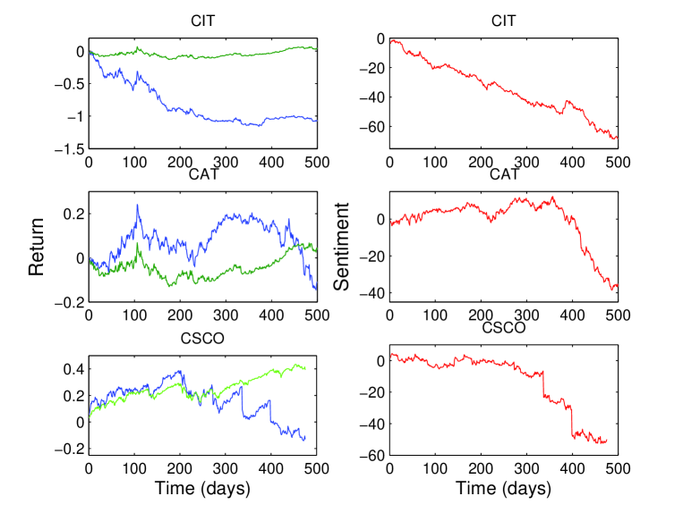
Figure 3: The figure shows the cumulative sentiment for three different stocks, Citi Bank, Caterpilar in the time period (03/01/2000 to 20/06/2008) and Cisco in the time period (01/06/2009 to 02/06/2011). The plots to the left shows in green the return of the Dow Jones and in blue the given stock over the given time period.

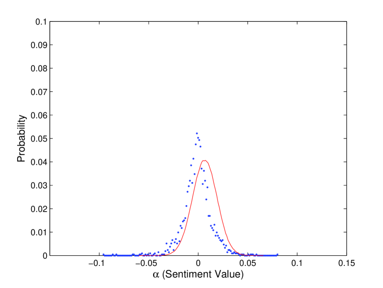
Figure 4: Probability distribution function of the sentiment variable $\alpha_{i}$.

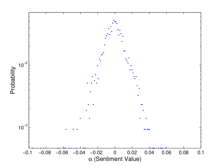
Figure 5: This figure is inset to figure 3.

References

- (1) H. Shefrin “A Behavioral Approach to Asset Pricing”, Academic Press Advanced Finance Series (2008), Chapter 15.
- (2) K. L. Fisher and M. Statman “Investor Sentiment and Stock Returns”, Financial Analysts Journal, 56, 2, 16-23 (Mar/Apr 2000).
- (3) M. Baker and J. Wurgler, “Investor Sentiment and the Cross-Section of Stock Returns” , The Journal of Finance, 61 (4), 1645-1680 (2006). doi:10.111/j.1540-6261.2006.00885.x.
- (4) G. W. Brown and M. T. Cliff, “Investor Sentiment and the Near-Term Stock Market” ,Journal of Empirical Finance, 11 (1), 1-27 (2002). doi:16/j.jempfin.2002.12.001.
- (5) P. Tetlock “Giving Content to Investor Sentiment: The Role of Media in the Stock Market” , The Journal of Finance Vol. LXII, NO. 3, p. 1139-1168, (June 2007).
- (6) J. B. De Long, A. Schleifer, L. H. Summers and R. J. Waldmann “Noise Trader Risk in Financial Markets”, , J. Polit. Econ., 98, 703-738, (1990).
- (7) J. B. De Long, A. Schleifer, L. H. Summers and R. J. Waldmann “The Survival of Noise Traders in Financial Markets”, , J. Bus., 64, 1-19, (1991).
- (8) W. Antweiler and M. Z. Frank “Is All That Talk Just Noise? The Information Content of Internet Stock Message Boards”, The Journal of Finance, Vol. 59, NO. 3, p. 1259-1294, (June 2004).
- (9) W. F. Sharpe, “Capital Asset Prices: A Theory of Market Equilibrium Under Conditions of Risk”, Journal of Finance, 19 (3), 425-442 (1964); J. Lintner, “The Valuation of Risk Assets and the Selection of Risky Investments in Stock Portfolios and Capital Budgets”, Review of Economics and Statistics, 47 (1), 13-37 (1965); J. Mossin, “Equilibrium in a Capital Asset Market”, Econometrica, Vol. 34, No. 4, 768-783 (1966).
- (10) J. Vitting Andersen, “Detecting Anchoring in Financial Markets”, Journal of Behavioral Finance, 11, 2, 129-33, (2010).
- (11) A. D. Baddeley, M. Eysenck and M. C. Anderson, “Memory”. Howe: Psychology Press (2009).
- (12) N. Miller and D. T. Campbell, “Recency and Primacy in Persuasion as a Function of Timing of Speeches and Measurements”, Journal of Abnormal and Social Psychology, 59, 1-9 (1959).
- (13) A. Tversky and D. Kahneman, “Judgment under Uncertainty: Heuristics and Biases”, Science 185, 1124-1131 (1974).
- (14) W. F. Sharpe, “Mutual Fund Performance”, Journal of Business 39 (S1): 119-138 (1966).
- (15) Taking the risk free return used in the usual definition of the Sharpe ratio, equal to 0.
- (16) With the risk free return equal 0.
- (17) The data used to construct figure 1 was taken from 1/1/2000 till 20/6/2008.
- (18) N. Barberis, A. Shleifer and R. Vishny, “A Model of Investor sSntiment”, in : R. Thaler (ed.) “Advances in Behavioral Finance. Vol. II. Princeton University Press (2005).