Determining the DNA stability parameters for the breathing dynamics of heterogeneous DNA by stochastic optimization

Abstract

We suggest that the thermodynamic stability parameters (nearest neighbor stacking and hydrogen bonding free energies) of double-stranded DNA molecules can be inferred reliably from time series of the size fluctuations (breathing) of local denaturation zones (bubbles). On the basis of the reconstructed bubble size distribution, this is achieved through stochastic optimization of the free energies in terms of Simulated Annealing. In particular, it is shown that even noisy time series allow the identification of the stability parameters at remarkable accuracy. This method will be useful to obtain the DNA stacking and hydrogen bonding free energies from single bubble breathing assays rather than equilibrium data.

I Introduction

The Watson-Crick double-helical form of DNA watson is not a static structure: even at standard salt conditions and room temperature the base pairs may intermittently open up and expose the otherwise protected core of the nucleotides. Such local denaturation bubbles are usually quite short-lived, however, the propensity of double-stranded DNA towards formation of longer-lived bubbles can be increased by elevating temperature or lowering the salt concentration. wartell ; frank ; dp ; Cant ; Gros In naturally underwound circular DNA denaturation bubbles are stabilized by partial twist release, jozef ; strick while in modern single DNA molecule setups bubble formation may be facilitated by the exertion of longitudinal stretching forces. pant ; rief ; busta ; hanke ; huguet The preferred location of bubbles is connected with the stability landscape of the genome, as quantified by maps of stability parameters, which are functions of the specific, underlying sequence of GC and AT base pairs. slucia ; blake ; krueger ; everaers ; blossey ; huguet In a biological context, bubbles correspond to so-called DNA Unwinding Elements (DUE), which are central in processes such as gene regulation, DNA replication, and transcription. sinden Similarly, in higher organisms the thermodynamic stability landscape of DNA is related to the coding versus non-coding properties of the genome. yeramian ; carlon The denaturation of a long DNA chain from double-strand to two separate single-strands is a physical phase transition, whose order is determined by the magnitude of the critical exponent $c$ for the entropy loss of a flexible polymer loop, see the discussion below. frank ; dp ; fisher ; wartell ; kafri ; hanke ; Gros The opening-closing dynamics of denaturation bubbles can be quantified by simple nonequilibrium models based on the gradient of the DNA stability free energy landscape. hanke1 ; bicout ; fogedby ; kafri1 ; novotny

Melting profiles of DNA can be obtained from a host of experimental techniques. These include UV spectroscopic methods, Cant circular dichroism, Cant fluorescence resonant energy transfer measurements, Gelf calorimetry, Sen or nuclear magnetic resonance, gueron among others. Single DNA manipulation techniques such as unzipping have recently been shown to provide high accuracy results for the stability parameters and their salt dependence. huguet From the respective melting or unzipping curves the DNA stability parameters are deduced, which in bioinformatics serve to predict the melting profiles of arbitrary, given DNA sequences. Zuk Up until now the different sets of stability parameters differ considerably from each other. slucia ; blake ; krueger ; everaers ; blossey ; huguet Alternative methods to measure these may help to pin down optimized parameters. One way could be to use dynamic information from bubble breathing. Indeed, by fluorescence correlation spectroscopy the breathing dynamics of single DNA bubbles has been monitored, producing the breathing-induced fluorescence-fluorescence correlation function, that is pronouncedly non-exponential. altan ; skb Given the recent progress in experimental methods, we expect that time series of single bubble dynamics will soon become available, in which opening or closing events of individual base pairs can be monitored. A high potential for such time records lies in nano-channel approaches as the one reported in Ref. jonas, , after new labeling techniques will become available shortly.

In what follows we pursue the question whether the bubble size distribution obtained from single breathing time series may, in principle, be used to obtain reliable information on the DNA stability parameters. We show that indeed by stochastic analysis methods such as Simulated Annealing (SA) accurate estimates for the stability parameters may be obtained for known DNA sequences.

The paper is structured as follows. We first introduce the general statistical model of DNA base pairing, before proceeding to present the methodology of SA. In the subsequent section we present our results, before drawing our conclusions.

II Statistical model for DNA denaturation

II.1 Thermodynamics

The size of denaturation bubbles typically ranges from a few broken base pairs (bps) at physiological temperature in linear, unconstrained DNA, to some 200 broken bps closer to the melting temperature of the DNA. wartell ; dp ; frank ; krueger ; skb Bubbles of some hundred broken base pairs also occur in naturally underwound DNA. jozef ; sinden Following the notation of Ref. krueger, , the stability of DNA is characterized by the free energies $\epsilon_{hb}(\rm AT)$ and $\epsilon_{hb}(\rm GC)$ for the Watson-Crick hydrogen bonds between complementary nucleotides (A and T, G and C, respectively) as well as the independent stacking free energies $\epsilon_{st}$ for disrupting the stacking interactions between nearest neighbor bps. These stacking energies depend on the nature of the two vicinal bps, as well as on their orientation along the DNA molecule ($3^{\prime}$ to $5^{\prime}$). The free energies are functions of temperature and salt concentration. Depending on the used set of stability parameters more or less pronounced asymmetries in the stacking free energies are observed. slucia ; blake ; krueger ; everaers ; blossey ; huguet In addition to the hydrogen bonding and stacking free energies, there is an additional energetic cost for initiating a bubble in the first place. Roughly speaking, this term originates from the fact that two stacking contacts need to be broken, while only one single broken bp yields an entropic gain. This is either taken into consideration by the cooperativity factor $\sigma_{0}$, or the so-called ring factor $\xi$, see below. REMM

The L33B9 sequence zeng we are analyzing in the present work is given as follows,

$$\begin{array}[]{l}\mathtt{5^{\prime}-cCGCCAGCGGCCTTTACTAAAGGCCGCTGCGCc-3^{\prime}},\end{array}$$ (1)

where the double-strand is completed by adding the complementary single strand. The sequence (1) is linear, and the high content of more stable GC bps at the two ends ensures that these ends preferentially remain closed. A denaturation bubble forms in the center of the chain that is rich in weaker AT bonds. We therefore view the two extremities denoted by the lower case symbol c as completely clamped. Labeling the sequence of bps by the coordinate $x$, ranging from $x=0$ to $x=M+1$, we thus have $M=31$ internal bps, which are allowed to open up, while the bps at $x=0$ and $x=M+1$ remain closed by definition. In a mathematical sense, the bps at the two extremities represent reflecting boundary conditions. Furthermore, we call $x_{L}$ and $x_{R}$ the momentary positions of the two closed bps embracing the denaturation bubble to the left and right, such that the bubble size becomes $m=x_{R}-x_{L}-1$. In terms of the Boltzmann factors for hydrogen bonding of the bp at position $x$,

$$u_{hb}(x)=\exp\left(\frac{\epsilon_{\mathrm{hb}}(x)}{k_{B}T}\right),$$ (2)

and the stacking interactions between the bps at positions $x-1$ and $x$,

$$u_{st}(x)=\exp\left(\frac{\epsilon_{\mathrm{st}}(x)}{k_{B}T}\right),$$ (3)

the bubble partition function becomes ($m\geqslant 1$):

$$\mathscr{Z}(x_{L},m)=\frac{\xi^{\prime}}{(1+m)^{c}}\prod_{x=x_{L}+1}^{x_{L}+m}u_{\mathrm{hb}}(x)\prod_{x=x_{L}+1}^{x_{L}+m+1}u_{\mathrm{st}}(x).$$ (4)

At $m=0$, we take $\mathscr{Z}(m=0)=1$. In Eq. (4), the factor $(1+m)^{-c}$ takes care of the entropy loss upon formation of a closed polymer loop. For a self-avoiding chain in three dimensions, the critical exponent becomes $c=1.76$ .fisher Corrections of $c$ may occur due to interactions with the rest of the chain, kafri however, for the short DNA construct used here, such effects are not expected to be relevant. The ring factor is $\xi\approx 10^{-3}$, krueger and we define $\xi^{\prime}=2^{c}\xi$. The ring factor may be interpreted as the cooperativity parameter, divided by the Boltzmann factor for stacking, $\xi=\sigma_{0}/\exp(\epsilon_{\mathrm{st}}/k_{B}T)$. krueger In principle, the ring factor depends on the position. However, a bubble will statistically always form at the weakest link. Considering this we have used a constant value of ring factor, $\xi$ in the present work. With above notation, the equilibrium distribution for finding a bubble of size $m$ and with the leftmost broken bp located at position $x+1$, is given by

$$P_{\mathrm{eq}}(x_{L},m)=\frac{\mathscr{Z}(x_{L},m)}{\mathscr{Z}(0)+\sum_{m=1}^{M}\sum_{x_{L}=0}^{M-m}\mathscr{Z}(x_{L},m)}.$$ (5)

II.2 Nonequilibrium: bubble breathing

Powered by thermal fluctuations, the bubble size becomes a random process as a function of time. Varying stepwise by further unzipping of one bp at position $x_{L}$ or $x_{R}$, or by zipping at $x_{L}+1$ and $x_{R}-1$, the bubble size $m$ performs a random walk along the coordinate $x$, the bubble breathing dynamics. hanke1 ; fogedby ; kafri1 ; skb ; bicout ; novotny This process is described by the master equation skb

$$\frac{\partial P(x_{L},m,t)}{\partial t}=\mathbb{W}P(x_{L},m,t),$$ (6)

where $P(x_{L},m,t)$ is the probability distribution for finding a bubble of size $m$ with the leftmost open bp at position $x_{L}+1$, at time $t$. The matrix $\mathbb{W}$ contains the transfer rates for all possible transitions in the $(x_{L},m)$ space, for details see Ref. skb, . In the long time limit, the solution $P$ of the master equation (6) equilibrates to the distribution $P_{\mathrm{eq}}$ of Eq. (5). To generate individual bubble breathing time series for $m(t)$ and $x_{L}(t)$, as well as construct the distribution $P_{\mathrm{eq}}$, one may employ the Gillespie algorithm. dtg ; suman

Following the experimental setup in Ref. altan, , one may study the dynamics of a tagged bp located at $x=x_{T}$. In the typical experimental scenario fluorescence occurs if the bps in a $\delta$-neighborhood of the fluorophore position $x_{T}$ are open. Measured fluorescence time series thus correspond to the stochastic variable $I(t)$, with the properties $I(t)=1$ if at least all bps in $(x_{T}-\delta,x_{T}+\delta)$ are open, and $I(t)=0$ otherwise. skb In what follows we probe whether a single bp is open or closed, i.e., we choose $\delta=0$.

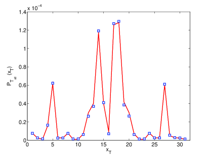
Figure 1: (Color online) Theoretical probability distribution for finding a tagged bp at position $x_{T}$ open (solid line), compared with the result from the converged SA scheme (blue open squares). The underlying DNA sequence is given in Eq. (1).

III Stochastic optimization

Given the probability distribution $P_{\mathrm{eq}}(m,x_{L})$, constructed from an experimental or simulations time series $m(t)$, $x_{L}(t)$, for a bubble in the DNA construct under consideration: can we reliably extract the stability parameters? Here we show that stochastic optimization is the method of choice.

Finding system parameters in a complex landscape is a generic task across disciplines. Fogar ; Pulay ; Sch ; Head ; Wales ; Bacelo ; Berne Typically, a given problem is cast in such a manner that the seeked-for optimum corresponds to an extremum of a functional in the complex search space. For instance, to obtain the global minimum in a rugged potential energy surface, one starts from any arbitrary point on this landscape and then moves on in the search space, following certain rules, such as accepting a move if the gradient norm for the new position decreases. This process converges to a point for which the gradient norm is zero. To verify whether this point is a minimum, one needs to check if the eigenvalues of the Hessian matrix at that point are all positive. A completely deterministic optimization procedure such as this minimization of the gradient norm, however, will generally fail to determine the global minimum if the search space features multiple minima. Once a local minimum is found, the deterministic search method will simply terminate. Such a misguidance is avoided by true global optimizers, whose search is not solely driven by a gradient. In particular, stochastic optimization techniques turn out to be very successful. Originally proposed by Kirkpatrick and coworkers to solve the traveling salesman problem, ksk1 ; ksk2 SA represents such a true global optimizer, and has been applied to a broad range of problems across disciplines, see, for instance, Refs. Car, ; Nandy, ; PDutta, ; Ming, ; Zuck, ; Aarts, ; Noller, ; Kalb, ; Franc, . In SA, the search space is initially sampled at a high temperature ($T_{\mathrm{at}}$). The associated thermal fluctuations at a suitable value of $T_{\mathrm{at}}$ will lift the optimizer out of local minima such that the search may continue towards increasingly deeper minima. Once the temperature becomes sufficiently small and/or the search is carried out over a sufficient time span, the entire search space is probed. Due to this ergodic property the global minimum is indeed found unequivocally. ksk2

Typically, an SA analysis is started at a sufficiently high temperature. This makes nearly all moves acceptable, as the criterion for accepting or rejecting a move is determined by the Metropolis criterion. In our case, the associated cost function, which is being minimized, is the sum of the squares of the difference of the occupation probabilities at the various positions,

$${\rm cost}_{i}=\sum_{i=1}^{M}(P_{\mathrm{eq}}(x_{i})-P_{T_{\mathrm{at}}}(x_{i}))^{2},$$ (7)

where $P_{T_{\mathrm{at}}}(x)$ denotes the distribution at position $x$ found in the current SA step, when the simulation temperature is $T_{\mathrm{at}}$. If, on going from one SA step ($i$) to the next ($i+1$) the magnitude of the cost function decreases, we at once accept that move. If it increases, we do not discard the move rightout. Instead, we subject it to the Metropolis test metrop : if the quantity $\Delta={\rm cost}_{i}-{\rm cost}_{i-1}$ has a positive value, the probability for accepting the move is determined by the function

$$F=\exp\left(-\frac{\Delta}{T_{\mathrm{at}}}\right).$$ (8)

For positive $\Delta$, $F$ is always between 0 and 1. For each evaluation of $F$, we invoke a random number $\mathrm{rand}$ between 0 and 1. If $F>\mathrm{rand}$, we accept the move. If not, the move is rejected. Thus, at very high $T_{\mathrm{at}}$, $F$ will be close to 1 and most moves will be accepted, such that a greater region of the search space will be sampled. As the simulation proceeds, $T_{\mathrm{at}}$ is decreased by the annealing schedule. Once the correct path towards the global minimum is followed, we need not search the entire space and concentrate on a small region, which will guide us specifically to the global minimum. That is, as $T_{\mathrm{at}}$ is lowered, a decreasing number of moves pass the Metropolis test. Ultimately, in our problem we recover the stability parameters from the SA analysis.

In SA, the crucial factor which determines the success of optimization is the annealing schedule, which is basically the rate at which the simulation temperature is decreased in successive annealing steps. In the present study we have kept the initial temperature at 1000. The rate of cooling was kept at $10\%$ of the value of the present step. We have also ensured that after every 30 SA steps, the system is re-heated to the initial starting value, i.e., the simulation temperature is forcibly increased to a higher value. This is done to remove any possibility of being trapped in a local minimum (coming out of which will be difficult if the simulation temperature is low). In successive SA steps, along with the temperature, the individual stability parameters are changed by the following strategy. If $u$ is a parameter chosen for change in SA, it is updated by the rule: $u^{{}^{\prime}}=u+u\times(-1)^{n}\times\delta\times r_{n}$, where $n$ is a random integer, $\delta$ is the amplitude of allowed change (kept at $0.01$), and $r_{n}$ is a random number between $0$ and $1$. The new $u{{}^{\prime}}$ (changed stability parameter) is used to generate the updated distribution profile. The magnitudes of the different optimization parameters are collected in Table 1.

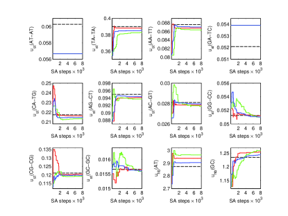
Figure 2: (Color online) Evolution of the free energy parameters of hydrogen bonding and base stacking as function of SA steps (full lines) from three separate SA runs. The black dashed horizontal lines represent the expected experimental values taken from Ref. krueger, , towards which convergence is expected to occur. Note the different scales on the vertical axes. The values for two pairs of bps, AT-AT and GA-TC, do not change in the SA procedure; these two pairs do not occur in the underlying sequence (1) and are thus not subject to the SA optimization criteria, i.e., they do not converge.

Table 1: Magnitude of optimization parameters used in SA.

Parameter	Magnitude
Annealing Schedule	$10\%$
Initial Simulation Temperature	1000
Magnitude of Change $\delta$	0.01

IV Results and Discussion

In a first step, the equilibrium distribution for a tagged bp at location $x_{T}$ in the DNA sequence (1) was determined from the theoretical stability parameters from Ref. krueger, . SA was then employed for successive convergence of $P_{T_{\mathrm{at}}}$ to this theoretical distribution through variation of the 12 independent free energy parameters (compare Table 2), by minimizing the cost function. The SA analysis was terminated once the value of the cost function becomes smaller than $10^{-4}$. Fig. 1 shows the quite accurate convergence of the SA scheme in terms of the equilibrium distribution.

To visualize the progress of the SA procedure, we display in Fig. 2 the progress of the approximation of the twelve DNA stability parameters of hydrogen bonding and base stacking (compare also Table 2) for 8000 SA steps, for three separate SA runs starting with different initial simulation temperatures. For each simulation the initial free energy values are chosen via random perturbation of the experimental $u$ values, krueger following our SA strategy. In all cases the convergence is quite accurate. Two parameters do not change during the SA scheme, these correspond to the two pairs of bps, that do not occur in the employed sequence (1). To be sure that the search proceeds without being held up in local basins, the annealing temperature was raised after every 30 SA steps and then allowed to follow the usual annealing schedule. The sudden jumps in the profile are a result of this effort. At an abruptly elevated temperature, newer moves start to get accepted and hence the zigzag pattern.

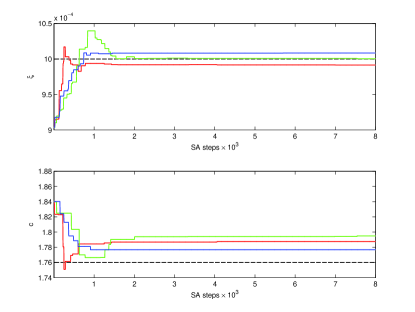
Figure 3: (Color online) Evolution of ring factor $\xi$ and critical exponent $c$ from three different SA runs. The black dashed horizontal lines represent the expected literature value towards which convergence is expected to occur.

In terms of the free energy values for hydrogen bonding and base stacking, the average results from 1000 SA runs are shown in Table 2. We also indicate which combinations of nearest neighbor pairs actually occur in the underlying sequence (1). The convergence of the SA algorithm in all cases is quite remarkable. In addition to the free energy parameter we also optimized the loop exponent $c$ and the ring factor $\xi$. The resultant simulation profiles (Fig. 3) show a good convergence towards theoretical values.

In typical experimental data the distribution of the bubble opening probability will be noisy, due to finite sampling and measurement errors. To check if our SA algorithm is robust against such noise we randomly perturbed the theoretically expected equilibrium distribution by a gaussian random processes with amplitude and width being the $P_{eq}$ and 10$\%$ of $P_{eq}$, respectively. Fig. 4 shows how this noisy data was quickly smoothened out to reach the theoretical distribution profile. We show snapshots of the process for different SA steps. In each figure, the original noisy data, the equilibrium distribution profile and the evolving profile at the particular SA step are shown. At 1500 SA steps, the noisy data completely matches with the equilibrium distribution.

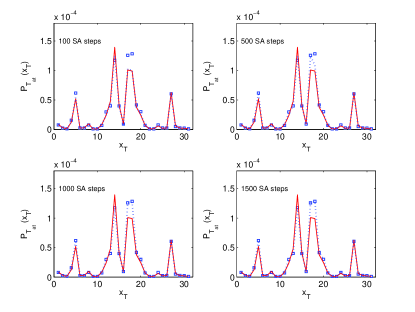
Figure 4: (color online) Plot of $P_{T_{\mathrm{at}}}(x_{T})$ against $x_{T}$ at various SA steps. In each panel the red solid lines represents the original noisy data, and the blue dashed line is the output of SA runs. The blue open squares stand for the theoretical distribution $P_{\mathrm{eq}}(x_{T})$. The plot for 1,500 SA steps already matches quite well the expected distribution $P_{eq}(x_{T})$.

Table 2: Comparison of experimental krueger and simulated free energy data. Each simulation data is a mean of 1000 different SA outputs. The rightmost column shows the presence ($\surd$) or absence ($\times$) of particular free energies in sequence (1). Units of free energies ($\epsilon_{st}$ and $\epsilon_{hb}$) reported here are kcal/mol. The last two rows of the table gives a comparison of the ring factor $\xi$ and critical exponent $c$.

	Experimental	SA results
$\epsilon_{st}$ (AT-AT)	-1.729409	-1.767474	$\times$
$\epsilon_{st}$ (TA-TA)	-0.579800	-0.588968	$\surd$
$\epsilon_{st}$ (AA-TT)	-1.499484	-1.510239	$\surd$
$\epsilon_{st}$ (GA-TC)	-1.819371	-1.798201	$\times$
$\epsilon_{st}$ (CA-TG)	-0.939677	-0.922743	$\surd$
$\epsilon_{st}$ (AG-CT)	-1.455363	-1.462615	$\surd$
$\epsilon_{st}$ (AC-GT)	-2.199241	-2.175124	$\surd$
$\epsilon_{st}$ (GG-CC)	-1.829370	-1.801741	$\surd$
$\epsilon_{st}$ (CG-CG)	-1.299554	-1.318516	$\surd$
$\epsilon_{st}$ (GC-GC)	-2.559130	-2.549840	$\surd$
$\epsilon_{hb}$ (AT)	0.649775	0.651781	$\surd$
$\epsilon_{hb}$ (GC)	0.129955	0.113848	$\surd$
$\xi$	0.001	0.001034062
c	1.76	1.758298

V Conclusion

Generalising our previous approach, obdyn we here demonstrate the outstanding ability of stochastic optimization to determine the stability parameters of double-stranded DNA from time series of the breathing dynamics of individual bps. Even for a short DNA sequence such as L33B9 [Eq. (1)] with only 31 internal bps, the convergence of the chosen SA scheme to all present base stacking and hydrogen bonding free energies is recovered with appreciable accuracy. Even when the input data are perturbed randomly, mimicking noisy experimental or simulations data, the stochastic optimization technique works successfully.

Optimization based on the bubble distribution $P_{\mathrm{eq}}(x)$ is not the only way to extract the DNA stability parameters. For instance, one might use average values for the zipping and unzipping rates of individual bps and relate their ratio to the underlying free energy difference. Alternatively, once from high throughput fluorescence correlation experiments an accurate result for the fluorescence autocorrelation function becomes available, one might use this function as basis for the optimization. In principle, one might also modify our approach to analyse data from DNA unzipping. This, however, requires detailed knowledge on the change of the stacking and hydrogen free energies upon stretching of the DNA strands.

In general, it may be worthwhile to also explore the possibility to apply other techniques such as the genetic algorithm, Gold parallel tempering, Earl or ant colony optimization, Dorigo ; Bon and to compare these methods.

- (1) J. D. Watson and F. H. C. Crick, Nature 171, 737 (1953); R. E. Franklin and R. G. Gosling, Nature 171, 740 (1953); F. Crick, Nature 227, 561 (1970).
- (2) M. D. Frank-Kamenetskii, Phys. Rep. 288, 13 (1997).
- (3) R. M. Wartell and A. S. Benight, Phys. Rep. 126, 67 (1985).
- (4) A. Y. Grosberg and A. R. Khokhlov, Statistical Physics of Macromolecules (AIP Press, New York, 1994).
- (5) D. Poland and H. A. Scheraga, Theory of Helix-Coil Transitions in Biopolymers (Academic Press, New York, 1970).
- (6) C. R. Cantor and P. R. Schimmel, Biophysical Chemistry (W H Freeman, New York, 1980).
- (7) T. R. Strick, V. Croquette, and D. Bensimon, Nature 404, 901 (2000).
- (8) J.-H. Jeon, J. Adamczik, G. Dietler, and R. Metzler, Phys. Rev. Lett. 105, 208101 (2010).
- (9) M. C. Williams, J. R. Wenner, I. Rouzina, and V. A. Bloomfield, Biophys. J. 80, 874 (2001); K. R. Chaurasiya, T. Paramanathan, M. J. McCauley, and M. C. Williams, Phys. Life Rev. 7, 299 (2010).
- (10) M. Rief, H. Clausen-Schaumann, and H. E. Gaub, Nature Struct. Biol. 4, 153 (1997); H. Clausen-Schaumann, M. Rief, C. Tolksdorf, and H. E. Gaub, Biophys. J. 78, 1997 (2000).
- (11) S. B. Smith, Y. J. Cui, and C. Bustamante, Science 271, 795 (1996).
- (12) A. Hanke, M. G. Ochoa, and R. Metzler, Phys. Rev. Lett. 100, 018106 (2008).
- (13) J. M. Huguet, C. V. Bizarro, N. Forns, S. B. Smith, C. Bustamante, and F. Ritort, Proc. Natl. Acad. Sci. USA 107, 15431 (2010).
- (14) A. Krueger, E. Protozanova, and M. D. Frank-Kamenetskii, Biophys. J. 90, 3091 (2006). The parametrisation of the DNA stability free energies in this work makes it possible to distinguish the stacking and the hydrogen bonding free energies.
- (15) R. D. Blake, J. W. Bizzaro, J. D. Blake, G. R. Day, S. G. Delcourt, J. Knowles, K. A. Marx, and J. SantaLucia, Jr., Bioinformatics 15, 370 (1999).
- (16) J. SantaLucia, Jr., Proc. Natl. Acad. Sci. U.S.A. 95, 1460 (1998).
- (17) D. Jost and R. Everaers, Biophys. J. 96, 1056 (2009).
- (18) R. Blossey and E. Carlon, Phys. Rev. E 68, 061911 (2003).
- (19) R. R. Sinden, DNA Structure and Function (Academic Press, San Diego, CA, 1994).
- (20) E. Carlon, M. L. Malki, and R. Blossey, Phys. Rev. Lett. 94, 178101 (2005).
- (21) E. Yeramian, Gene 255, 139 (2000).
- (22) M. E. Fisher, J. Chem. Phys. 44, 616 (1966).
- (23) Y. Kafri, D. Mukamel, and L. Peliti, Phys. Rev. Lett. 85, 4988 (2000); Euro. Phys. J. B 27, 132 (2002).
- (24) A. Hanke and R. Metzler, J. Phys. A 36, L473 (2003).
- (25) D. Bicout and E. Kats, Phys. Rev. E 70, 010902(R) (2004).
- (26) A. Bar, Y. Kafri, and D. Mukamel, Phys. Rev. Lett. 98, 038103 (2007).
- (27) T. Novotný, J. N. Pedersen, T. Ambjörnsson, M. S. Hansen, and R. Metzler, Europhys. Lett. 77, 48001 (2007); J. N. Pedersen, M. S. Hansen, T. Novotný, T. Ambjörnsson, and R. Metzler, J. Chem. Phys. 130, 164117 (2009).
- (28) H. C. Fogedby and R. Metzler, Phys. Rev. Lett. 98, 070601 (2007); Phys. Rev. E 76, 061915 (2007).
- (29) C. A. Gelfand, G. E. Plum, S. Mielewczyk, D. P. Remeta and K. J. Breslauer, Proc. Natl. Acad. Sci. U. S. A. 96, 6113 (1999)
- (30) M. M. Senior, R. A. Jones K. J. Breslauer, Proc. Natl. Acad. Sci. U. S. A. 85, 6242 (1988)
- (31) M. Géron, M. Kochoyan, and J.-L. Leroy, Nature 328, 89 (1987).
- (32) M. Zuker, Nucl. Acids Res. 31, 3406 (2003).
- (33) G. Altan-Bonnet, A. Libchaber, and O. Krichevsky, Phys. Rev. Lett. 90, 138101 (2003).
- (34) T. Ambjörnsson, S. K. Banik, O. Krichevsky and R. Metzler, Phys. Rev. Lett. 97, 128105 (2006); Biophys. J. 92, 2674 (2007); T. Ambjörnsson, S. K. Banik, M. A. Lomholt and R. Metzler, Phys. Rev. E 75, 021908 (2007).
- (35) W. Reisner, N. B. Larsen, A. Silahtaroglu, A. Kristensen, N.Tommerup, J. O. Tegenfeldt, and H. Flyvbjerg, Proc. Natl. Acad. Sci. USA 107, 13294 (2010).
- (36) Note that the bubble will on average open at the weakest base pair-base pair couple. The ring factor or cooperativity constant is therefore independent of the index .
- (37) Y. Zeng, A Montrichok, and G. Zocchi, J. Mol. Biol. 339, 67 (2004).
- (38) D. T. Gillespie, J. Comput. Phys. 22, 403 (1976); J. Phys. Chem. 81, 2340 (1977).
- (39) S. K. Banik, T. Ambjörnsson, and R. Metzler, Europhys. Lett. 71, 852 (2005).
- (40) G. Fogarsi and P. Pulay, Ann. Rev. Phys. Chem. 35, 191 (1984).
- (41) P. Pulay and J. Simons, eds., Geometrical Derivatives of Energy Surfaces and Molecular Properties (Reidel, Dordecht, 1986).
- (42) H. B. Schlegel, Adv. Chem. Phys. 67, 249 (1987).
- (43) J. D. Head, B. Weiner and M. C. Zerner, Int. J. Quant. Chem. 33, 177 (1988).
- (44) M. C. Prentiss, D. J. Wales and P. G. Wolynes, J. Chem. Phys. 128, 225106 (2008).
- (45) D. E. Bacelo and S. E. Fioressi, J. Chem. Phys. 119, 11695 (2003).
- (46) P. Liu and B. J. Berne, J. Chem. Phys. 118, 2999 (2003).
- (47) K. S. Kirkpatrick, C. D. Gelatt, and M. P. Vecchi, Science 220, 671 (1983).
- (48) K. S. Kirkpatrick, J. Stat. Phys. 34, 975 (1984).
- (49) R. Car and M. Parinello, Phys. Rev. Lett. 55, 2471 (1985).
- (50) S. Nandy, P. Chaudhury, R. Sharma and S. P. Bhattacharyya, J. Theor. Comp. Chem. 7, 977 (2008).
- (51) P. Dutta, D. Mazumdar and S. P. Bhattacharyya, Chem. Phys. Lett. 181, 288 (1991).
- (52) J. Mingjun and T. Huanwen, Chaos Solitons Fractals, 21, 933 (2004).
- (53) E. Lyman and D. M. Zuckerman, J. Chem. Phys. 127, 065101 (2007).
- (54) P. J. M. van Laarhoven and E. H. L. Aarts, Simulated Amnnealing Theory and Applications (Kluwer Academic, Dordecht, Holland 1987).
- (55) A. Korostelev, M. Laurberg and H. F. Noller, Proc. Natl. Acad. Sci. U. S. A. 106, 18195 (2009).
- (56) A. Moglich, D. Weinfurtner, T. Maurer, N. Gronwald and H. R.Kalbitzer, BMC Bioinformatics 6, 91 (2005).
- (57) D. Francois, Ann. Appl. Prob. 12, 248 (2002).
- (58) N. Metropolis, A. W. Rosenbluth, M. N. Rosenbluth, A. H. Teller and E. Teller, J. Chem. Phys. 21, 1087 (1953).
- (59) P. Chaudhury, R. Metzler, and S. K. Banik, J. Phys. A 42, 335101 (2009).
- (60) D. E. Goldberg, Genetic Algorithms in Search, Optimization and Machine Learning (Addison Wesley, Rading, MA, 1989).
- (61) D. J. Earl and M. W. Deem, Phys. Chem. Chem. Phys. 7, 3910 (2005).
- (62) M. Dorigo, V. Maniezzo and A. Colorni, IEEE Transactions on Systems, Man and Cybernetics - Part - B: CYBERNETICS 26, 29 (1996).
- (63) E. Bonabeau, M. Dorigo, and G. Theraulaz, Nature 406, 39 (2000).