Flux tubes in the SU(3) vacuum

Abstract:

We analyze the distribution of the chromoelectric field generated by a static quark-antiquark pair in the SU(3) vacuum. We find that the transverse profile of the flux tube resembles the dual version of the Abrikosov vortex field distribution and give an estimate of the London penetration length in the confined vacuum.

1 Introduction

Color confinement in Quantum Chromo-Dynamics (QCD) is a long-distance behavior whose understanding continues to be a challenge for theoretical physics [1, 2]. Tube-like structures emerge by analyzing the chromoelectric field between static quarks [3, 4, 5, 6, 7, 8, 9, 10, 11, 12, 13, 14, 15, 16, 17, 18, 19]. Such tube-like structures naturally lead to linear potential and consequently to a “phenomenological” understanding of color confinement. To explain the formation of chromoelectric flux tubes in QCD vacuum, ’t Hooft [20] and Mandelstam [21] proposed the hypothesis that QCD vacuum behaves like a coherent state of color magnetic monopoles, which leads to the picture of QCD vacuum a magnetic (dual) superconductor [22]. According to this picture the observed color flux tubes are naturally accounted for by the (dual) Meissner effect, in analogy with the formation of Abrikosov tubes in the usual superconductivity [23]. Even if the ’t Hooft construction does not explain the dynamical formation of color magnetic monopoles, many lattice calculations [24, 25, 26, 27, 28, 29, 30, 31, 32] have given numerical evidence in favor of magnetic monopole condensation in the QCD vacuum.

On the other side, magnetic monopole condensation could be the consequence rather than the origin of the confinement mechanism [33]. Even in this case, however, the dual superconductivity picture provides us with a “phenomenological” frame for the analysis of tube-like structure in the QCD vacuum.

The outcome of previous studies [12, 13, 14, 15, 16] of the SU(2) confining vacuum was the following: (1) presence in lattice configurations of color flux tubes made up by the chromoelectric fields directed along the line joining a static quark-antiquark pair; (2) transverse size of the chromoelectric flux tube interpreted as the London penetration length in the Meissner effect; (3) penetration length measured both in the maximal Abelian gauge and without gauge fixing, with compatible results, thus supporting gauge-invariance; (4) determination of the string tension as the energy stored into the flux tube per unit length, in good agreement with the results in the literature.

The aim of the present work is to extend the analysis to the more interesting case of the SU(3) gauge theory.

2 Color fields on the lattice

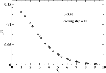
Figure 1: (Left) The connected correlator (1) between the plaquette $U_{p}$ and the Wilson loop. The subtraction appearing in the definition of correlator is not explicitly drawn. (Right) Longitudinal component of the chromoelectric field versus the distance $x_{t}$ at $\beta=5.9$ after 10 cooling steps.

We use a connected correlator (Fig. 1)(left) to explore the field configurations produced by a static quark-antiquark pair ($N$ is the number of colors) [7, 8, 34, 35]:

$$\rho_{W}=\frac{\left\langle{\rm tr}\left(WLU_{P}L^{\dagger}\right)\right\rangle}{\left\langle{\rm tr}(W)\right\rangle}-\frac{1}{N}\,\frac{\left\langle{\rm tr}(U_{P}){\rm tr}(W)\right\rangle}{\left\langle{\rm tr}(W)\right\rangle}\;.$$ (1)

In the naive continuum limit [8]

$$\rho_{W}\stackrel{{\scriptstyle a\rightarrow 0}}{{\longrightarrow}}a^{2}g\left[\left\langle F_{\mu\nu}\right\rangle_{q\bar{q}}-\left\langle F_{\mu\nu}\right\rangle_{0}\right]\;,$$ (2)

so that

$$\hat{F}_{\mu\nu}(x)=\sqrt{\frac{\beta}{2N}}\,\rho_{W}(x)$$ (3)

The configuration with plaquette parallel to the Wilson loop leads to chromoelectric field longitudinal to the axis defined by the static quarks.

2.1 The case of SU(2) gauge theory

The case of the SU(2) gauge theory was studied in [10, 12, 13, 14, 15, 16]. The main result was that the flux tube is almost completely formed by the longitudinal chromoelectric field, $E_{l}$, which is constant along the flux and rapidly decreasing in the transverse direction $x_{t}$. In the dual Meissner effect interpretation, the transverse shape of $E_{l}$ is the dual version of the Abrikosov vortex field distribution [10, 12, 13, 14, 15, 16] and therefore must obey

$$E_{l}(x_{t})=\frac{\Phi}{2\pi}\mu^{2}K_{0}(\mu x_{t})\;,\;\;\;\;\;x_{t}>0\;,$$ (4)

where $\Phi$ is the external flux and $\lambda=1/\mu$ is the London penetration length (this is valid for $\lambda\gg\xi$, with $\xi$ the coherence length of a type-II superconductor).

In the past numerical study (lattices $16^{4}$, $20^{4}$ and $24^{4}$, statistics 20-100) [16] approximate scaling was found, $\mu/\sqrt{\sigma}=4.04(18)$ (i.e. $\lambda=0.118(5)$ fm for $\sqrt{\sigma}=420$ MeV). In this work ($20^{4}$ lattice, statistics $1000$), we find $\mu/\sqrt{\sigma}=4.21(16)$ – see Ref. [36] for details.

2.2 The case of SU(3) gauge theory

The main motivation for repeating the study in SU(3) is to verify the scaling of $\mu$ with the string tension and to compare the resulting determination of $\mu/\sqrt{\sigma}$ with SU(2). This result should provide us with important reference values, that any approach aiming at explaining confinement should be able to accommodate.

We performed numerical simulations with the Wilson action and periodic boundary conditions, using a the Cabibbo-Marinari algorithm [37], combined with overrelaxation on SU(2) subgroups. The summary of $\beta$ values, lattice size, Wilson loop size and statistics is given in Table 1. The lattice size $L$ has been chosen such that the combination $L\sqrt{\sigma}\gtrsim 4$. The size of the Wilson loop entering the definition of the operator given in Eq. (1) has been fixed at $L/2-2a$. In order to reduce the autocorrelation time, measurements were taken after 10 updatings. The error analysis was performed by the jackknife method over bins at different blocking levels.

$\beta$	lattice	Wilson loop	statistics
5.90	$18^{4}$	$7\times 7$	5.k
6.00	$20^{4}$	$8\times 8$	4.5k
6.05	$22^{4}$	$9\times 9$	3.6k
6.10	$24^{4}$	$10\times 10$	2.4k

Table 1: Summary of the Monte Carlo simulations.

In order to reduce the quantum fluctuations we adopted the controlled cooling algorithm. It is known [38] that by cooling in a smooth way equilibrium configurations, quantum fluctuations are reduced by a few order of magnitude, while the string tension survives and shows a plateau. We shall show below that the penetration length behaves in a similar way. The details of the cooling procedure are described in Ref. [16] for the case of SU(2). Here we adapted the procedure to the case of SU(3), by applying successively this algorithm to various SU(2) subgroups. The control parameter $\delta$ was fixed at the value 0.0354, as in Ref. [16].

A novelty with respect to the study of Ref. [16] is related with the construction of the lattice operator given in Eq. (1). If the Wilson loop lies on the plane, say, 1-2, then the Schwinger line can leave the plane 1-2 in the direction, say, 3; before attaching the plaquette to the Schwinger line, the latter can be prolongated further in the direction 4, by one or two links. In this way, by varying the length of the Schwinger line in the direction 3, one can obtain a large set of distances $x_{t}/a$ between the center of the plaquette and the center of the Wilson loop, both integer and non-integer. On each configuration we averaged over all possible directions for the relative orientation of the Wilson loop to the Schwinger line.

The general strategy underlying this work is the following: (1) for each $\beta$ we generate an ensemble of thermalized configurations and, correspondingly, ensembles of “cooled” configurations after a number of cooling steps ranging from 5 to 16; (2) for different values of the distance $x_{t}$, the longitudinal component of the chromoelectric field, averaged over each cooled ensemble of configurations, is then determined by means of the operator (1), with the help of Eq. (3) (see, for example, Fig. 1(right), which shows $E_{l}(x_{t})$ averaged over the ensemble at $\beta=5.90$ after 10 cooling steps); (3) for each cooling step, data for $E_{l}(x_{t})$ are fitted with the function given in Eq. (4) and the parameters $\mu$ and $\Phi$ are extracted; (4) a plateau is then searched in the plot for $\mu$ and $\Phi$ versus the cooling step.

In Table 2 we report the results for $a\mu$ of the fit at the four $\beta$ values considered in this work for one selected cooling step. The table with the results for the other fit parameter, $\Phi$, can be found in Ref. [36]. When the fit is done on all available data for $E_{x}(x_{t})$, above a certain $x_{t,{\rm{min}}}$, the $\chi^{2}$/d.o.f. is very high, thus reflecting the wiggling of data due to the inclusion of non-integer distances $x_{t}/a$. When the fit is restricted to integer values of $x_{t}/a$, the $\chi^{2}$/d.o.f. turns out to be very reasonable. Remarkably, the resulting parameters obtained with the two fitting procedures agree very well.

In Figs. 2 we show the behavior of $a\mu$ and $\Phi$ with the cooling step at $\beta=6.05$. Similar figures for the other values of $\beta$ are given in Ref. [36]. A short plateau is visible, except for the case of $\mu$ at $\beta=5.90$. We take as “plateau” value for $\mu$ the value corresponding to the number of cooling steps given in the second column of Table 2.

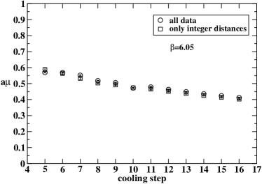
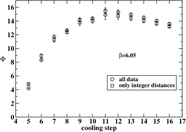
Figure 2: (Left) The inverse of the penetration length $a\mu$ at $\beta=6.05$ versus the cooling step. Data are obtained by fitting the transverse profile of the longitudinal chromoelectric field with the function (4); circles correspond to fit to all available data of $E_{l}(x_{t})$ starting from a certain $x_{t,{\rm min}}$, while squares correspond to fit of $E_{l}(x_{t})$ for integer values of $x_{t}/a$. (Right) The same for the amplitude of the longitudinal chromoelectric field $\Phi$.

$\beta$	cooling step	$a\mu$	$\chi^{2}$/d.o.f.	$x_{t,\rm{min}}/a$	data set
5.90	10	0.5577(12)	626.	6	all data
6.00	9	0.51015(92)	383.	6	all data
6.05	10	0.4730(13)	133.	7	all data
6.10	10	0.4357(20)	27.	7	all data
5.90	10	0.5557(40)	1.22	7	integer $x_{t}/a$
6.00	9	0.5099(28)	2.56	9	integer $x_{t}/a$
6.05	10	0.4735(39)	1.08	8	integer $x_{t}/a$
6.10	10	0.4349(56)	0.25	8	integer $x_{t}/a$

Table 2: Summary of the fit values for $a\mu$.

Finally, we studied the scaling of the “plateau” values of $a\mu$ with the string tension. For this purpose, we have expressed these values of $a\mu$ in units of $\sqrt{\sigma}$, using the parameterization

$$a\sqrt{\sigma}(g)=f_{SU(3)}(g^{2})[1+0.2731\,\hat{a}^{2}(g)-0.01545\,\hat{a}^{4}(g)+0.01975\,\hat{a}^{6}(g)]/0.01364\;,$$ (5)

$$\hat{a}(g)=\frac{f_{SU(3)}(g^{2})}{f_{SU(3)}(g^{2}(\beta=6))}\;,\;\;\;\beta=\frac{6}{g^{2}}\,,\;\;\;5.6\leq\beta\leq 6.5\;,$$

$$f_{SU(3)}(g^{2})=\left({b_{0}g^{2}}\right)^{-b_{1}/2b_{0}^{2}}\,\exp\left(-\frac{1}{2b_{0}g^{2}}\right)\,,\;\;\;\;\;b_{0}=\frac{11}{(4\pi)^{2}}\;,\;\;\;b_{1}=\frac{102}{(4\pi)^{4}}\;,$$ (6)

given in Ref. [39].

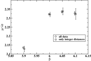
Figure 3: Scaling of the inverse London penetration length with $\sqrt{\sigma}$ versus $\beta$. Data have been slightly shifted on the horizontal axis for the sake of readability.

Figure 3 suggests that the ratio $\mu/\sqrt{\sigma}$ displays a nice plateau in $\beta$, as soon as $\beta$ is larger than 6. The scaling of $\mu$ is a natural consequence of the fact that the penetration length is a physical quantity related to the size $D$ of the flux tube [10, 12], $D\simeq 2/\mu$. We get as estimate for the penetration length in SU(3) gauge theory, $\mu/\sqrt{\sigma}=2.325(5)$, corresponding to $\mu$ = 0.977(2) GeV. We observe that this value is in nice agreement with the determinations of Ref. [40], obtained by using correlators of plaquette and Wilson loops not connected by the Schwinger line, thus leading to the (more noisy) squared chromoelectric and chromomagnetic fields.

We note that the ratio between the penetration lengths for the SU(2) gauge theory and the SU(3) gauge theory is $\mu_{\text{SU(2)}}/\mu_{\text{SU(3)}}$ = 1.81(7). This result recalls analogous behavior seen in a different study of SU(2) and SU(3) vacuum in a constant external chromomagnetic background field [41]. In Ref. [41] numerical evidence that the deconfinement temperature for SU(2) and SU(3) gauge systems in a constant Abelian chromomagnetic field decreases when the strength of the applied field increases was given. Moreover, as discussed in Refs. [27, 41, 42], above a critical strength $\sqrt{gH_{c}}$ of the chromomagnetic external background field the deconfined phase extends to very low temperatures. It was found [41] that the ratio between the critical field strengths for SU(2) and SU(3) gauge theories is $\sqrt{gH_{c}}|_{\text{SU(2)}}/\sqrt{gH_{c}}|_{\text{SU(3)}}$ = 2.03(17), in remarkable agreement with the ratio between the penetration lengths for SU(2) and SU(3). As stressed in the Conclusions of Ref. [41], the peculiar dependence of the deconfinement temperature on the strength of the Abelian chromomagnetic field $gH$ could be naturally explained if the vacuum behaved as a disordered chromomagnetic condensate which confines color charges due both to the presence of a mass gap and the absence of color long range order, such as in the Feynman picture for Yang-Mills theory in (2+1) dimensions [43]. The circumstance that ratio between the SU(2) and SU(3) penetration lengths agrees within errors with the above discussed ratio of the critical chromomagnetic fields, suggests us that the Feynman picture of the Yang-Mills vacuum could be a useful guide to understand the dynamics of color confinement.

References

- [1] M. Bander, Phys. Rept. 75, 205 (1981).
- [2] J. Greensite, Prog. Part. Nucl. Phys. 51, 1 (2003).
- [3] M. Fukugita and T. Niuya, Phys. Lett. B132, 374 (1983).
- [4] J.E. Kiskis and K. Sparks, Phys. Rev. D30, 1326 (1984).
- [5] J.W. Flower and S.W. Otto, Phys. Lett. B160, 128 (1985).
- [6] J. Wosiek and R.W. Haymaker, Phys. Rev. D36, 3297 (1987).
- [7] A. Di Giacomo et al., Phys. Lett. B236, 199 (1990).
- [8] A. Di Giacomo et al., Nucl. Phys. B347, 441 (1990).
- [9] V. Singh et al, Phys. Lett. B306, 115 (1993).
- [10] P. Cea and L. Cosmai, Nucl. Phys. Proc. Suppl. 30, 572 (1993).
- [11] Y. Matsubara et al., Nucl. Phys. Proc. Suppl. 34, 176 (1994).
- [12] P. Cea and L. Cosmai, Nuovo Cim. A107, 541 (1994).
- [13] P. Cea and L. Cosmai, Nucl. Phys. Proc. Suppl. 34, 219 (1994).
- [14] P. Cea and L. Cosmai, Phys. Lett. B349, 343 (1995).
- [15] P. Cea and L. Cosmai, Nucl. Phys. Proc. Suppl. 42, 225 (1995).
- [16] P. Cea and L. Cosmai, Phys. Rev. D52, 5152 (1995).
- [17] G.S. Bali et al., Phys. Rev. D51, 5165 (1995).
- [18] R.W. Haymaker and T. Matsuki, Phys. Rev. D75, 014501 (2007).
- [19] A. D’Alessandro et al., Nucl. Phys. B774, 168 (2007).
- [20] G. ’t Hooft, in High Energy Physics, EPS International Conference, Palermo, 1975, edited by A. Zichichi (1975).
- [21] S. Mandelstam, Phys. Rept. 23, 245 (1976).
- [22] G. Ripka, hep-ph/0310102.
- [23] A.A. Abrikosov, Soviet Physics JETP 5, 1174 (1957).
- [24] H. Shiba and T. Suzuki, Phys. Lett. B351, 519 (1995).
- [25] N. Arasaki et al., Phys. Lett. B395, 275 (1997).
- [26] P. Cea and L. Cosmai, Phys. Rev. D62, 094510 (2000).
- [27] P. Cea and L. Cosmai, JHEP 11, 064 (2001).
- [28] A. Di Giacomo et al., Phys. Rev. D61, 034503 (2000).
- [29] A. Di Giacomo et al., Phys. Rev. D61, 034504 (2000).
- [30] J.M. Carmona et al., Phys. Rev. D64, 114507 (2001).
- [31] P. Cea et al., JHEP 02, 018 (2004).
- [32] A. D’Alessandro et al., Phys. Rev. D81, 094501 (2010).
- [33] G. ’t Hooft, hep-th/0408183.
- [34] D.S. Kuzmenko and Y.A. Simonov, Phys. Lett. B494, 81 (2000).
- [35] A. Di Giacomo et al., Phys. Rept. 372, 319 (2002).
- [36] M.S. Cardaci et al., Phys. Rev. D83, 014502 (2011).
- [37] N. Cabibbo and E. Marinari, Phys. Lett. B119, 387 (1982).
- [38] M. Campostrini et al., Phys. Lett. B225, 403 (1989).
- [39] R.G. Edwards et al., Nucl. Phys. B517, 377 (1998).
- [40] P. Bicudo et al., PoS LATTICE2010, 268 (2010).
- [41] P. Cea and L. Cosmai, JHEP 08, 079 (2005).
- [42] P. Cea et al., JHEP 12, 097 (2007).
- [43] R.P. Feynman, Nucl. Phys. B188, 479 (1981).