Introduction to Loop Quantum Cosmology

Introduction to Loop Quantum Cosmology

Kinjal BANERJEE ^†, Gianluca CALCAGNI ^‡ and Mercedes MARTÍN-BENITO ^‡

K. Banerjee, G. Calcagni and M. Martín-Benito

^† Department of Physics, Beijing Normal University, Beijing 100875, China kinjalb@gmail.com

^‡ Max Planck Institute for Gravitational Physics (Albert Einstein Institute),
^‡ Am Mühlenberg 1, D-14476 Golm, Germany calcagni@aei.mpg.de, mercedes@aei.mpg.de

Received September 30, 2011, in final form March 13, 2012; Published online March 25, 2012

This is an introduction to loop quantum cosmology (LQC) reviewing mini- and midisuperspace models as well as homogeneous and inhomogeneous effective dynamics.

loop quantum cosmology; loop quantum gravity

83C45; 83C75; 83F05

Introduction

General relativity (GR) and quantum mechanics are two of the best verified theories of modern physics. While general relativity has been spectacularly successful in explaining the universe at astronomical and cosmological scales, quantum mechanics gives an equally coherent physical picture on small scales. However, one of the biggest unfulfilled challenges in physics remains to incorporate the two theories in the same framework. Ordinary quantum field theories, which have managed to describe the three other fundamental forces (electromagnetic, weak and strong), have failed for general relativity because it is not perturbatively renormalizable.

Loop quantum gravity (LQG) [14, 111, 170, 186] is an attempt to construct a mathematically rigorous, non-perturbative, background independent formulation of quantum general relativity. GR is reformulated in terms of Ashtekar–Barbero variables, namely the densitized triad and the Ashtekar connection. The basic classical variables are taken to be the holonomies of the connection and the fluxes of the triads and these are then promoted to basic quantum operators. The quantization is not the standard Schrödinger quantization but an unitarily inequivalent choice known as loop/polymer quantization. The kinematic structure of LQG has been well developed. A robust feature of LQG, not imposed but emergent, is the underlying discreteness of space.

With the aim of obtaining physical implications from LQG, in the last years the application of loop quantization techniques to cosmological models has undergone a notable development. This field of research is known under the name of loop quantum cosmology (LQC). The models analyzed in LQC are mini- and midisuperspace models. These models have Killing vectors which reduce the degrees of freedom of full GR. In the case of minisuperspaces, the reduced theories have no field-theory degrees of freedom remaining. Although there are field-theory degrees of freedom in the midisuperspace models, their number is smaller than in the full theory. Therefore, these are simplified systems which provide toy models suitable for studying some aspects of the full quantum gravity theory. Moreover, classical solutions are well known (in fact, we are aware of very few systems which have closed-form solutions of Einstein equations with no Killing vectors) and it is relatively easy to study the effects of the quantization.

LQC cannot be considered the cosmological sector of LQG because the symmetry reduction is carried out before quantizing, and the results so obtained may not be the same if the reduction is done after quantization. However by adapting the techniques used in the full theory to the symmetry-reduced cosmological models we may hope to capture some of the crucial features of the full theory, as well as to obtain hints about how to tackle them. Indeed, one of the generic characteristics of LQC is the avoidance of the classical singularity. In the present absence of recognized experimental and observational signatures of quantum gravity, this novel and robust result has been increasing the hope that LQG may indeed be the correct theory of quantum gravity.

In this article we will review the progress made in the various cosmological models studied in LQC in the last few years. A recent review [24] emphasizes aspects that are only briefly mentioned here, such as the “simplified” or “solvable” LQC framework, the details of effective dynamics for FRW models with non-zero curvature and/or cosmological constant, and inflationary perturbation theory in LQC. On the other hand, here we focus more on midisuperspaces and discuss lattice refinement parametrizations at some length. Before starting, we shall briefly recall the main features in the kinematic structures of LQG. Similar ingredients are used in the kinematic structure of the LQC models to be discussed later.

1 Loop quantization

1.1 Ashtekar–Barbero formalism

In the Hamiltonian formulation, the four-dimensional spacetime metric is described by a three-metric $q_{ab}$ induced in the spatial sections $\Sigma$ that foliate the spacetime manifold, the lapse function $N$ and the shift vector $N^{a}$ [1, 160]. Both the lapse $N$ and the shift vector $N^{a}$ are Lagrange multipliers accompanying the constraints that encoded the general covariance of general relativity. These constraints are, respectively, the scalar or Hamiltonian constraint and the diffeomorphisms constraint (which is a three-vector). Therefore, the physically relevant information is encoded in the spatial three-metric and in its canonically conjugate momentum, or equivalently, in the extrinsic curvature $K_{ab}=\mathcal{L}_{n}q_{ab}/2$, where $n$ is the unit normal to $\Sigma$ and $\mathcal{L}_{n}$ is the Lie derivative along $n$ [196].

LQG is based in a formulation of general relativity as a gauge theory [3, 5, 6, 172, 173], in which the phase space is described by a $su(2)$ gauge connection, the Ashtekar–Barbero connection $A^{i}_{a}$, and its canonically conjugate momentum, the densitized triad $E^{a}_{i}$, that plays the role of an “electric field”. To define these objects, first one introduces the co-triad $e^{i}_{a}$, defined as $q_{ab}=e^{i}_{a}e^{j}_{b}\delta_{ij}$, where $\delta_{ij}$ stands for the Kronecker delta in three dimensions, and then one defines the triad, $e^{a}_{i}$, as its inverse $e^{a}_{i}e^{j}_{b}=\delta_{i}^{j}\delta^{a}_{b}$. The densitized triad then reads $E^{a}_{i}=\sqrt{q}e^{a}_{i}$, where $q$ stands for the determinant of the spatial three-metric. In turn, the Ashtekar–Barbero connection reads [30] $A^{i}_{a}=\Gamma^{i}_{a}+\gamma K^{i}_{a}$, where $\gamma$ is an arbitrary real and non-vanishing parameter, called the Immirzi parameter [123, 124], $K^{i}_{a}=K_{ab}e^{b}_{j}\delta^{ij}$ is the extrinsic curvature in triadic form, and $\Gamma^{i}_{a}$ is the spin connection compatible with the densitized triad. Namely, it verifies $\nabla_{b}E^{a}_{i}+\epsilon_{ijk}\Gamma^{j}_{b}E^{ak}=0$, where $\epsilon_{ijk}$ is the totally antisymmetric symbol and $\nabla_{b}$ is the usual spatial covariant derivative [196]. The canonical pair $(A,E)$ has the following Poisson bracket:

$$\{A^{a}_{i}(x),E^{j}_{b}(y)\}=8\pi G\gamma\delta^{a}_{b}\delta^{j}_{i}\delta(x-y),$$

where $G$ is Newton constant and $\delta(x-y)$ denotes the three-dimensional Dirac delta distribution on the hypersurface $\Sigma$.

Since the internal Euclidean metric $\delta_{ij}$ is invariant under $SU(2)$ rotations, the internal $SU(2)$ degrees of freedom are gauge. Therefore, in this formulation of general relativity, besides the diffeomorphisms constraint $\mathcal{C}_{a}$ and the scalar (or Hamiltonian) constraint $\mathcal{C}$, there is a gauge (or Gauss) constraint $\mathcal{G}_{i}$ fixing the rotation freedom that we have just introduced. In the variables $(A^{a}_{i},E^{j}_{b})$, those constraints have the following expression (in vacuum) [186],

$$\mathcal{G}_{i}=\partial_{a}E^{a}_{i}+\epsilon_{ijk}\Gamma^{j}_{a}E^{ak}=0,$$

$$\mathcal{C}_{a}=F_{ab}^{i}E^{b}_{i}=0,$$

$$\mathcal{C}=\frac{1}{\sqrt{|\det(E)|}}\epsilon_{ijk}\left[F^{i}_{ab}-(1+\gamma^{2})\epsilon^{i}_{mn}K^{m}_{a}K^{n}_{b}\right]E^{aj}E^{bk}=0,$$

where $F^{i}_{ab}$ is the curvature tensor of the Ashtekar–Barbero connection,

$$F^{i}_{ab}=\partial_{a}A^{i}_{b}-\partial_{b}A^{i}_{a}+\epsilon_{ijk}A^{j}_{a}A^{k}_{b}.$$

1.1.1 Holonomy-flux algebra

The next step is to define the holonomies and fluxes which will later be promoted to basic quantum variables.

The configuration variables chosen are the holonomies of $A^{i}_{a}$. They are more convenient than the connection itself thanks to their properties under gauge transformation. The holonomy of the connection $A$ along the edge $e$ is given by

$$h_{e}(A)=\mathcal{P}e^{\int_{e}dx^{a}A^{i}_{a}(x)\tau_{i}},$$

where $\mathcal{P}$ denotes path ordering and $\tau_{i}$ are the generators of $SU(2)$, such that $[\tau_{i},\tau_{j}]=\epsilon_{ijk}\tau^{k}$.

The momentum conjugate to the holonomy is given by the flux of $E^{a}_{i}$ over surfaces $S$ and smeared with a $su(2)$-valued function $f^{i}$:

$$E(S,f)=\int_{S}f^{i}E^{a}_{i}\epsilon_{abc}dx^{b}dx^{c}.$$

The description of the phase space in terms of holonomies and fluxes is not only suitable for its transformation properties, but also because these objects are diffeomorphism invariant and their definition is background independent. Moreover, their Poisson bracket is divergence-free

$$\{E(S,f),h_{e}(A)\}=2\pi G\gamma\epsilon(e,S)f^{i}\tau_{i}h_{e}(A),$$

where $\epsilon(e,S)$ represents the regularization of the Dirac delta: it vanishes if $e$ does not intersect $S$, as well as if $e\subset S$, and $|\epsilon(e,S)|=1$ if $e$ and $S$ intersect in one point, the sign depending on the relative orientation between $e$ and $S$ [14].

1.2 Kinematic Hilbert space

In LQG, the holonomy-flux algebra is represented over a kinematical Hilbert space that is different from the more familiar Schrödinger-type Hilbert space. It is given by the completion of the space of cylindrical functions (defined on the space of generalized connections) with respect to the so-called Ashtekar–Lewandowski measure [13, 15, 17, 27]. We give a very brief description of this kinematical Hilbert space below, while the details can be found in [14, 111, 170, 186] (and references therein).

A generalized connection $h_{e}(A)\equiv\bar{A}_{e}$ is an assignment of $\bar{A}\in$ $SU(2)$ to any analytic path $e\subset\Sigma$. A graph $\Gamma$ is a collection of analytic paths $e\subset\Sigma$ meeting at most at their endpoints. We will consider only closed graphs. The point at which two edges meet is called a vertex. Let n be the number of edges in $\Gamma$. A function cylindrical with respect to $\Gamma$ is given by

$$\psi_{\Gamma}(\bar{A}):=f_{\Gamma}\big{(}\bar{A}_{e_{1}},\dots,\bar{A}_{e_{n}}\big{)},$$

where $f_{\Gamma}$ is a smooth function on $SU(2)^{n}$. The space of states cylindrical with respect to $\Gamma$ are denoted by Cyl_Γ. The space of all functions cylindrical with respect to some $\Gamma\in\Sigma$ is denoted by Cyl and is given by

$$\mbox{Cyl}=\bigcup_{\Gamma}\mbox{Cyl}_{\Gamma}.$$

Given a cylindrical function $\psi_{\Gamma}(\bar{A})\in{\rm Cyl}$, the Ashtekar–Lewandowski measure, denoted by $\mu_{0}$, is defined by

$$\int_{\overline{{\mathcal{A}}}}d\mu_{0}[\psi_{\Gamma}(\bar{A})]:=\int_{SU(2)^{n}}\prod_{e\subset\Gamma}dh^{e}f_{\Gamma}\big{(}\bar{A}_{e_{1}},\dots,\bar{A}_{e_{n}}\big{)},\qquad\forall\,\psi_{\Gamma}(\bar{A}),$$

where d$h$ is the normalized Haar measure on $SU(2)$. Using this measure we can define an inner product on Cyl:

$$\langle\psi_{\Gamma},\psi_{\Gamma}^{\prime}\rangle:=\langle f_{\Gamma}\big{(}\bar{A}_{e_{1}},\dots,\bar{A}_{e_{n}}\big{)},g_{\Gamma^{\prime}}\big{(}\bar{A}_{e_{1}},\dots,\bar{A}_{e_{m}}\big{)}\rangle$$

$$\phantom{\langle\psi_{\Gamma},\psi_{\Gamma}^{\prime}\rangle}{}=\int_{SU(2)^{n}}\prod_{e\subset\Xi_{\Gamma\Gamma^{\prime}}}dh^{e}\overline{f_{\Gamma}\big{(}\bar{A}_{e_{1}},\dots,\bar{A}_{e_{n}}\big{)}}g_{\Gamma^{\prime}}\big{(}\bar{A}_{e_{1}},\dots,\bar{A}_{e_{m}}\big{)},$$

where ${\Xi}_{\Gamma\Gamma^{\prime}}$ is any graph such that $\Gamma\subset\Xi_{\Gamma\Gamma^{\prime}}$ and $\Gamma^{\prime}\subset\Xi_{\Gamma\Gamma^{\prime}}$. Then, the kinematical Hilbert space of LQG is the Cauchy completion of Cyl in the Ashtekar–Lewandowski norm: ${\mathcal{H}}_{\rm kin}=L^{2}(\overline{{\mathcal{A}}},d\mu_{0})$.

A basis on this Hilbert space is provided by spin network states, which are constructed as follows. Given a graph $\Gamma$, each edge $e$ is colored by a non-trivial irreducible representation $\pi_{j_{e}}$ of $SU(2)$. Spin network states are cylindrical functions with respect to this colored graph. They are denoted by $T_{s}:=T_{\Gamma,\vec{j}}(\bar{A})$ where $\vec{j}=\{j_{e}\}$. Then, every cylindrical function can be expanded in the basis of spin network states.

On $\mbox{Cyl}_{\Gamma}$ the operators representing the corresponding holonomies act by multiplication, while the operator representing the flux is given by

$$\hat{E}_{\Gamma}(S,f)=i2\pi G\hbar\sum_{e\subset\Gamma}\epsilon(e,S)\text{Tr}\left(f^{i}\tau_{i}\bar{A}_{e}\frac{\partial}{\partial\bar{A}_{e}}\right).$$

To obtain the quantum version of the more general operators, they have to be first rewritten in terms of the basic holonomy-flux operators. Note that the quantum configuration space is not the space of smooth connections but rather the space of holonomies (or generalized connections). Since the Ashtekar–Lewandowski measure is discontinuous in the connection, there is no well-defined operator for the connection on ${\mathcal{H}}_{\rm kin}$. Consequently, the curvature must be defined in terms of holonomies before it can be promoted to a quantum operator. The strategy in the full theory is to define any general quantum operator via regularization as follows (see [14, 186] for details):

• the spatial manifold $\Sigma$ is triangulated into elementary tetrahedra;

• the integral over $\Sigma$ is replaced by a Riemann sum over the cells;

• for each cell, we define a regularized expression in terms of the basic operators, such that we get the correct classical expression in the limit the cell is shrunk to zero;

• this is promoted to a quantum operator provided it is densely defined on ${\mathcal{H}}_{\rm kin}$.

In the subsequent sections we shall see how the same strategy is applied for defining the quantum operators in LQC. One significant difference is that in the full theory the final expressions are independent of the regularization, while in the symmetry-reduced models the regularization (i.e., the size of the cells) cannot be removed and has to be treated as an ambiguity. However, we can fix the form of the ambiguity by taking hints from the full theory.

One of the most interesting features of LQG is that the spectra of the operators representing geometrical quantities like area and volume are discrete. Discrete eigenvalues imply that the underlying spatial manifold is also discrete at least when we are close to the quantum gravity scale. This is a feature of the quantization scheme and it also plays and important role in the singularity avoidance in LQC minisuperspace models.

This is the kinematical structure of LQG. However we are interested in physical states, i.e. states which are annihilated by the all the constraints. To obtain the physical Hilbert space we now need to solve the quantum constraints. The Gauss constraint is easy to solve and we can obtain gauge invariant Hilbert space spanned by the gauge invariant spin networks. The infinitesimal diffeomorphism constraint cannot be expressed as a self-adjoint operator on ${\mathcal{H}}_{\rm kin}$. However we can consider finite diffeomorphisms and the solutions to the finite diffeomorphism constraint are obtained via group averaging. It turns out that these solutions do not lie in ${\mathcal{H}}_{\rm kin}$ but in Cyl^⋆, the algebraic dual of Cyl.

In the construction of the Hamiltonian constraint operator we face a number of problems (see [72] and references therein for details). Although a well-defined Hamiltonian constraint operator can be constructed which satisfies an on-shell anomaly-free quantum constraint algebra, the quantization procedure suffers from a number of ambiguities: in the choice of the regulators, in the transcription in terms of basic quantum variables, and in the choice of curvature approximants. Also the domain of the Hamiltonian constraint operator is not known. Efforts have been made to reduce the ambiguities by studying the off-shell closure of the constraint algebra and by trying to find the correct semiclassical limit, but no significant progress has been made so far. So, although we have a well-defined full quantum theory of gravity at the kinematical level, the physical Hilbert-space construction is beset by a number of open problems and is not yet complete.

LQC tries to study some of the features of Loop quantization while avoiding the problems of the full theory. As we shall see later, the programme of LQC tries to closely follow the same steps, as far as possible, in the much simpler case of cosmological models with no (or at most one) field-theory degrees of freedom. In minisuperspace models it is possible to go beyond the kinematics and construct the physical Hilbert space. Another useful procedure developed to study the effect of the underlying discreteness is the use of effective equations to study homogeneous cosmologies and perturbations therein. This has opened up a large number of systems to semiclassical analyses. It is hoped that lessons learned from LQC can give hints about how to tackle the issues being faced in LQG.

2 Plan of the review

Significant progress has been made in the study of a number of cosmologies in LQC. Here, we shall give an overall account of various facets of LQC, outlining technical aspects, reviewing the results achieved and indicating the directions of further research. The rest of the paper is divided into three parts.

In Part I we discuss LQC minisuperspace models. The simplest cases of minisuperspace are Friedmann–Robertson–Walker (FRW) models, which are homogeneous and isotropic. The kinematical quantization programme followed for these models will be discussed in detail, using the example of flat FRW. We also describe the results obtained in the physical Hilbert space including the dynamical singularity resolution and the bounce. Open and closed FRW models, with and without a cosmological constant, are briefly discussed. The next level of complication, Bianchi models, consists in removing the assumption of isotropy. In this case, our illustrative example will be the Bianchi I model but we also indicate the work done so far for Bianchi II and Bianchi IX cases.

Then, Part II focusses on the LQC of midisuperspace models which are neither homogeneous nor isotropic. We describe the only case whose loop quantization has been studied in some detail, the linearly polarized Gowdy $T^{3}$ model. Two contrasting approaches have been taken in the study of this model. In the first approach, the degrees of freedom have been separated into homogeneous and inhomogeneous sectors. The homogeneous sector is quantized using the tools developed in LQC, while the inhomogeneous sector is Fock quantized. In the second approach, the model is studied as a whole mimicking the steps of LQG. We describe and compare both procedures.

Finally, in Part III we discuss the programme of effective dynamics developed in LQC. In contrast to the previous two parts, this approach aims to incorporate the effects of the discrete geometry as corrections to the classical equations. In this way it may be possible to link LQC to phenomenological evidence.

In the end we summarize the current directions of ongoing research. This review is intended as an introduction of the main results achieved in the field in the past few years, especially in the Hamiltonian formalism, and it does not cover more recent work being done in the area of cosmological perturbations, phenomenology, and spin-foam cosmology. We will comment about these and other lines of research in Sections 9 and 10.

Part I Minisuperspaces in loop quantum cosmology

LQC [2, 4, 44, 149] adapts the techniques developed in loop quantum gravity [14, 170, 186] to the quantization of simpler models than the full theory, as minisuperspace models. Minisuperspace models are solutions of Einstein’s equations with a high degree of symmetry, so much so that there are no field theory degrees of freedom remaining. They lead to homogeneous cosmological solutions all of which suffer from a singularity where the classical equations of motion break down. Since, after quantization, these are essentially quantum mechanical systems, they serve as good toy models for testing the predictions of LQG.

In LQC, we start from the classically symmetry-reduced phase space and then try to apply the steps followed in LQG to these systems. Owing to simplifications due to classical symmetry reduction, many technical complications typical of LQG can be avoided, and the quantization programme can be carried out beyond what has been achieved so far in the full theory. The fact that there is a well-defined full theory which tells us that the underlying spatial geometry is discrete is a crucial ingredient in the formulation of LQC. A significant achievement of LQC is the development of a well-defined quantum theory for cosmological models where the classical singularity is absent. This resolution of the classical singularity is a robust feature of LQC as it is seen in all the minisuperspace models studied so far, as well as under various choices made in addressing the ambiguities arising in quantization. In this part we shall review the LQC of various known minisuperspace cosmological scenarios.

3 Friedmann–Robertson–Walker models

LQC started with the pioneering works by Bojowald [38, 46, 47, 48, 49], that showed the first attempts of implementing the methods of LQG to the quantization of the simplest cosmological model: the flat Friedmann–Robertson–Walker (FRW) model (homogeneous and isotropic with flat spatial sections), whose geometry is described by a single degree of freedom, the scale factor. This system, even if very simple, is physically interesting since, at large scales, our universe is approximately homogeneous and isotropic. In addition, cosmological observations are compatible with a spatially flat geometry.

After the early papers by Bojowald, the kinematic structure of LQC was revised and more rigorously established [9], which made it possible to complete the quantization of the model in presence of a homogeneous massless scalar field minimally coupled to the geometry, as well as to study the resulting quantum evolution [12, 19, 20, 21]. Classically, this model represents expanding universes with an initial big bang singularity, where certain physical observables, such as the matter density, diverge. Remarkably, the quantum dynamics resolves the singularity replacing it with a quantum bounce, while for semiclassical states it agrees with the classical dynamics far away form the singularity. Therefore, even though this is the simplest cosmological model, its loop quantization, also called polymeric quantization, already leads to relevant results, the most important one being the avoidance of the singularity.

Using the example of the flat FRW model coupled to a massless scalar, we shall discuss in detail the basics and the mathematical structure of LQC, adopting the so-called improved dynamics prescription [21].

3.1 Classical phase space description

3.1.1 Ashtekar–Barbero formalism

The classical phase space in the presence of homogeneity is much simpler than the general situation described in the introduction. In homogeneous cosmology, the gauge and diffeomorphisms constraints are trivially satisfied, the Hamiltonian constraint being the only survivor in the model. Moreover, for flat FRW the spin connection vanishes. In this case, the geometry part of the scalar constraint in its integral version is $C_{\text{grav}}(N)=NC_{\text{grav}}$, with

$$C_{\text{grav}}=\int_{\Sigma}d^{3}x\,\mathcal{C}=-\frac{1}{\gamma^{2}}\int_{\Sigma}d^{3}x\frac{\epsilon_{ijk}F^{i}_{ab}E^{aj}E^{bk}}{\sqrt{|\det(E)|}}.$$ (3.1)

Since flat FRW spatial sections $\Sigma$ are non-compact, and the variables that describe it are spatially homogeneous, integrals such as (3.1) diverge. To avoid that, one usually restricts the analysis to a finite cell $\mathcal{V}$. Owing to homogeneity, the study of this cell reproduces what happens in the whole universe. When imposing also isotropy, the connection and the triad can be described (in a convenient gauge) by a single parameter $c$ and $p$, respectively, in the form [9]

$$A^{i}_{a}=cV_{o}^{-1/3}\,{}^{o}e^{i}_{a},\qquad E^{a}_{i}=pV_{o}^{-2/3}\sqrt{{}^{o}q}\,{}^{o}e^{a}_{i}.$$

Here we have introduced a fiducial co-triad ${}^{o}e^{i}_{a}$ that we will choose to be diagonal, ${}^{o}e^{i}_{a}=\delta^{i}_{a}$, and the determinant $\sqrt{{}^{o}q}$ of the corresponding fiducial metric. The results do not depend on the fiducial choice. With the above definitions, the symplectic structure is defined via,

$$\{c,p\}=\frac{8\pi G\gamma}{3}.$$

The variable $p$ is related to the scale factor $a$ commonly employed in geometrodynamics through the expression $a(t)=\sqrt{|p(t)|}V_{o}^{-1/3}$. Note that $p$ is positive (negative) if physical and fiducial triads have the same (opposite) orientation.

On the other hand, a (homogeneous) massless scalar field $\phi$, together with its momentum $P_{\phi}$, provide the canonical pair describing the matter content, with Poisson bracket $\{\phi,P_{\phi}\}=1$. Then, the total Hamiltonian constraint contains a matter contribution beside the geometry one, given in equation (3.1), and reads

$$C=C_{\text{grav}}+C_{\text{mat}}=-\frac{6}{\gamma^{2}}c^{2}\sqrt{|p|}+8\pi G\frac{P_{\phi}^{2}}{V}=0,$$ (3.2)

where $V=|p|^{3/2}$ is the physical volume of the cell $\mathcal{V}$.

3.1.2 Holonomy-flux algebra

When defining holonomies and fluxes in LQC, and in the particular case of isotropic FRW models, owing to the homogeneity it is sufficient to consider straight edges oriented along the fiducial directions, and with oriented length equal to $\mu V_{o}^{1/3}$, where $\mu$ is an arbitrary real number. Therefore, the holonomy along one such edge, in the $i$-th direction, is given by

$$h_{i}^{\mu}(c)=e^{\mu c\tau_{i}}=\cos\left(\frac{\mu c}{2}\right)\mathbbm{1}+2\sin\left(\frac{\mu c}{2}\right)\tau_{i}.$$

Then, the gravitational part of the configuration algebra is the algebra generated by the matrix elements of the holonomies, namely, the algebra of quasi-periodic functions of $c$, that are the complex exponentials

$$\mathcal{N}_{\mu}(c)=e^{\frac{i}{2}\mu c}.$$

In analogy with the terminology employed in LQG [14, 186], the vector space of these quasi-periodic functions is called the space of cylindrical functions defined over symmetric connections, and it is denoted by $\text{Cyl}_{\text{S}}$.

In turn, the flux is given by

$$E(S,f)=pV_{o}^{-2/3}A_{S,f},$$

where $A_{S,f}$ is the fiducial area of $S$ times an orientation factor (that depends on $f$). Then, the flux is essentially described by $p$.

In summary, in isotropic and homogeneous LQC the phase space is described by the variables $\mathcal{N}_{\mu}(c)$ and $p$, whose Poisson bracket is

$$\{\mathcal{N}_{\mu}(c),p\}=i\frac{4\pi G\gamma}{3}\mu\mathcal{N}_{\mu}(c).$$

3.2 Kinematical structure

Mimicking the quantization implemented in LQG, in LQC we adopt a representation of the algebra generated by the phase space variables $\mathcal{N}_{\mu}(c)$ and $p$ that is not continuous in the connection, and therefore there is no operator representing $c$ [9]. More concretely, the quantum configuration space is the Bohr compactification of the real line, $\mathbb{R}_{\text{Bohr}}$, and the corresponding Haar measure that characterizes the kinematical Hilbert space is the so-called Bohr measure [192]. It is simpler to work in momentum representation. In fact, such Hilbert space is isomorphic to the space of functions of $\mu\in\mathbb{R}$ that are square summable with respect to the discrete measure [192], known as polymeric space. In other words, employing the kets $|\mu\rangle$ to denote the quantum states $\mathcal{N}_{\mu}(c)$, whose linear span is the space $\text{Cyl}_{\text{S}}$ (dense in $\mathbb{R}_{\text{Bohr}}$), the kinematical Hilbert space is the completion of $\text{Cyl}_{\text{S}}$ with respect to the inner product $\langle\mu|\mu^{\prime}\rangle=\delta_{\mu\mu^{\prime}}$. We will denote this Hilbert space by $\mathcal{H}_{\text{grav}}$. Note that $\mathcal{H}_{\text{grav}}$ is non-separable, since the states $|\mu\rangle$ form a non-countable orthogonal basis.

Obviously, the action of $\hat{\mathcal{N}}_{\mu}$ on the basis states is

$$\hat{\mathcal{N}}_{\mu^{\prime}}|\mu\rangle=|\mu+\mu^{\prime}\rangle.$$

On the other hand, the Dirac rule $[\hat{\mathcal{N}}_{\mu},\hat{p}]=i\hbar\widehat{\{\mathcal{N}_{\mu}(c),p\}}$ implies that

$$\hat{p}|\mu\rangle=p(\mu)|\mu\rangle,\qquad p(\mu)=\frac{4\pi l_{\text{Pl}}^{2}\gamma}{3}\mu,$$

where $l_{\text{Pl}}=\sqrt{G\hbar}$ is the Planck length. As we see, the spectrum of this operator is discrete, as a consequence of the representation not being continuous in $\mu$. Due to this lack of continuity, the Stone–von Neumann theorem about the uniqueness of the representation in quantum mechanics [180, 195] is not applicable in this context. Therefore, the loop quantization of this model is inequivalent to the standard Wheeler–DeWitt (WDW) quantization [99, 199], where operators have a typical Schrödinger-like representation. In fact, while the WDW quantization fails in solving the problem of the big bang singularity, the loop quantization is singularity free [20, 21], as we will see later.

For the matter field, we adopt a standard Schrödinger-like representation, with $\hat{\phi}$ acting by multiplication and $\hat{P}_{\phi}=-i\hbar\partial_{\phi}$ as derivative, being both operators defined on the Hilbert space $L^{2}(\mathbb{R},d\phi)$. As domain, we take the Schwartz space $\mathcal{S}(\mathbb{R})$ of rapidly decreasing functions, which is dense in $L^{2}(\mathbb{R},d\phi)$. The total kinematical Hilbert space is then $\mathcal{H}_{\text{kin}}=\mathcal{H}_{\text{grav}}\otimes L^{2}(\mathbb{R},d\phi)$.

3.3 Hamiltonian constraint operator

3.3.1 Curvature operator and improved dynamics

Since the connection is not well defined in the quantum theory, the classical expression of the Hamiltonian constraint, given in equation (3.2), cannot be promoted directly to an operator. In order to obtain the quantum analogue of the gravitational part, we follow the procedure adopted in the full theory. We start from the general expression (3.1) and express the curvature tensor in terms of the holonomies, which do have a well-defined quantum counterpart.

Following LQG, we take a closed square loop with holonomy

$$h^{\mu}_{\square_{ij}}=h_{i}^{\mu}h_{j}^{\mu}(h_{i}^{\mu})^{-1}(h_{j}^{\mu})^{-1},$$

that encloses a fiducial area $A_{\square}=\mu^{2}V_{o}^{2/3}$. The curvature tensor then reads [9]

$$F^{i}_{ab}=-2\;\lim_{A_{\square}\rightarrow 0}\text{tr}\left(\frac{h^{\mu}_{\square_{jk}}-\delta_{jk}}{A_{\square}}\tau^{i}\right){}^{o}e^{j}_{a}{}^{o}e^{k}_{b}.$$ (3.3)

This limit is classically well defined. However, in the quantum theory we cannot contract the area to zero because that limit does not converge.

Since we have a well defined full theory (unlike WDW quantization), we can appeal to the discretization of geometry coming from it. In LQG, geometric area has a discrete spectrum with a non-vanishing minimum eigenvalue $\Delta$ [16, 171]. This suggests that we should not take the null area limit, but consider only areas larger than $\Delta$. Then, we contract the area of the loop till a minimum value $A_{\square_{\min}}=\bar{\mu}^{2}V_{o}^{2/3}$, such that the geometric area corresponding to this fiducial area, given by the flux $E(\square_{\min},f=1)=p\bar{\mu}^{2}$, is equal to $\Delta$. In short, the curvature is defined by the regularized expression

$${F}^{i}_{ab}=-2\,\text{tr}\left(\frac{h^{\bar{\mu}}_{\square_{jk}}-\delta_{jk}}{\bar{\mu}^{2}V_{o}^{2/3}}\tau^{i}\right){}^{o}e^{j}_{a}{}^{o}e^{k}_{b},$$ (3.4)

where $\bar{\mu}$, characterizing the minimum area of the loop, is given by the Ansatz

$$\frac{1}{\bar{\mu}}=\sqrt{\frac{|p|}{\Delta}}.$$ (3.5)

This choice of $\bar{\mu}$ is usually called improved dynamics in the LQC literature [21]. Note that the smaller the value of $\bar{\mu}$ is, or equivalently the bigger the value of $|p|$ is, the better equation (3.4) approximates the classical expression (3.3), so that both expressions agree in the regime in which the area of the cell under study is large enough. Finally, the curvature operator is obtained by promoting equation (3.4) to an operator. Let us remark that there are two kinds of ambiguities in the definition of this operator. On the one hand, the value of the parameter $\bar{\mu}$, that is fixed by the improved dynamics prescription, as we have just explained. On the other hand, we also have the ambiguity in the $SU(2)$ representation we use for calculating the trace. As usual in LQC [44], we will compute the holonomies in the fundamental representation of spin $1/2$.

Note that terms of the kind ${\mathcal{N}}_{\bar{\mu}}=e^{i\bar{\mu}c/2}$ contribute to $h^{\bar{\mu}}_{\square_{ij}}$. In order to define the operator $\hat{\mathcal{N}}_{\bar{\mu}}=\widehat{e^{i\bar{\mu}c/2}}$, it is assumed that this operator generates unit translations over the affine parameter associated with the vector field $\bar{\mu}[p(\mu)]\partial_{\mu}$ [21]. In other words, we introduce a canonical transformation in the geometry sector of the phase space, such that it is described by the variable $b=\hbar\bar{\mu}c/2$ and its canonically conjugate variable $v(p)=(2\pi\gamma l_{\text{Pl}}^{2}\sqrt{\Delta})^{-1}\text{sgn}(p)|p|^{3/2}$ (sgn denotes the sign), with $\{b,v\}=1$. The variable $v(\mu)=v[p(\mu)]$ indeed verifies $\partial_{v}=\bar{\mu}(\mu)\partial_{\mu}$. Then, we relabel the basis states of $\mathcal{H}_{\text{grav}}$ with this new parameter $v$ that, unlike $\mu$, is adapted to the action of $\hat{\mathcal{N}}_{\bar{\mu}}$. In fact, introducing the operator $\hat{v}$ with action $\hat{v}|v\rangle=v|v\rangle$, it is straightforward to show that $\hat{\mathcal{N}}_{\bar{\mu}}|v\rangle=|v+1\rangle$, so that the Dirac rule $[\widehat{e^{ib/\hbar}},\hat{v}]|v\rangle=i\hbar\widehat{\{e^{ib/\hbar},v\}}|v\rangle$ is satisfied. On the other hand, we obtain $\hat{p}|v\rangle=(2\pi\gamma l_{\text{Pl}}^{2}\sqrt{\Delta})^{2/3}\text{sgn}(v)|v|^{2/3}|v\rangle$.

It is worth mentioning that the parameter $v$ has a geometrical interpretation: its absolute value is proportional to the physical volume of the cell $\mathcal{V}$, given by

$$\hat{V}=\widehat{|p|}^{3/2},\qquad\hat{V}|v\rangle=2\pi\gamma l_{\text{Pl}}^{2}\sqrt{\Delta}|v||v\rangle.$$

The quantization within the prescription (3.5) meant an important improvement for LQC [21]. Earlier, it was assumed that the minimum fiducial length was just some constant $\mu_{o}$ related to $\Delta$ [9]. However, the resulting quantum dynamics was not successful, inasmuch as the quantum effects of the geometry could be important at scales where the matter density was not necessarily high. In that case, in the semiclassical regime the physical results deviated significantly from the predictions made by general relativity [20]. Improved dynamics solves this problem. Furthermore, it has been proved that it is the only minisuperspace quantization (among a certain family of possibilities) yielding to a physically admissible model [92], independent of the fiducial structures, with a well-defined classical limit in agreement with GR, and giving rise to a scale of Planck order where quantum effects are important and solve the singularity problem.

3.3.2 Representation of the Hamiltonian constraint

When trying to promote the gravitational part of the scalar constraint (3.1) to an operator, we find an additional difficulty concerning the inverse of the volume,

$$\frac{1}{V}=\frac{\sqrt{{}^{o}q}}{\sqrt{|\det(E)|}V_{o}}.$$

The volume operator has a discrete spectrum with the eigenvalue zero included, so its inverse (obtained by using the spectral theorem) is not well defined in zero. Nonetheless, following LQG [185, 187], from the classical identity

$$\frac{\epsilon_{ijk}E^{aj}E^{bk}}{\sqrt{|\det(E)|}}=\sum_{k=1}^{3}\frac{\text{sgn}(p)}{2\pi\gamma GV_{o}^{1/3}}\frac{1}{l}\,{}^{o}e^{k}_{c}\,{}^{o}\epsilon^{abc}\,\text{tr}\big{(}h_{k}^{l}(c)\big{\{}[h_{k}^{l}(c)]^{-1},V\big{\}}\tau_{i}\big{)},$$ (3.6)

we can obtain an operator for the left-hand side of this expression by promoting the functions on the right-hand side to the corresponding operators, and by making the replacement $\widehat{\{\;\;,\;\;\}}\rightarrow-(i/\hbar)[\hat{\;\;},\hat{\;\;}]$. Note that the parameter $l$ labels a quantization ambiguity. In order not to introduce new scales in the theory, we take for $l$ the value $\bar{\mu}=\sqrt{{\Delta}/{|p|}}$ [21].

Plugging this result into the Hamiltonian constraint (3.1), as well as the curvature given in equation (3.4), we obtain that the geometry (or gravitational) contribution to the Hamiltonian constraint operator is [21]

$$\widehat{C}_{\text{grav}}=i\frac{3\widehat{\text{sgn}(p)}}{2\pi\gamma^{3}l_{\text{Pl}}^{2}\Delta^{3/2}}\hat{V}[\widehat{\sin\left(\bar{\mu}c\right)}\widehat{\text{sgn}(p)}]^{2}\big{(}\hat{\mathcal{N}}_{\bar{\mu}}\hat{V}\hat{\mathcal{N}}_{-\bar{\mu}}-\hat{\mathcal{N}}_{-\bar{\mu}}\hat{V}\hat{\mathcal{N}}_{\bar{\mu}}\big{)},$$ (3.7)

with

$$\widehat{\sin(\bar{\mu}c)}=\frac{\hat{\mathcal{N}}_{2\bar{\mu}}-\hat{\mathcal{N}}_{-2\bar{\mu}}}{2i}.$$

Let us now deal with the representation of the matter contribution, given in the second term of equation (3.2). To represent the inverse of the volume, we follow the same strategy as before, now starting with the classical identity

$$\frac{\text{sgn}(p)}{|p|^{1-s}}=\frac{1}{s4\pi\gamma G}\frac{1}{l}\text{tr}\left(\sum_{i}\tau^{i}h_{i}^{l}(c)\big{\{}[h_{i}^{l}(c)]^{-1},|p|^{s}\big{\}}\right).$$

As before, we take the trace in the fundamental representation and we choose $l$ equal to $\bar{\mu}$ in the quantum theory. To fix the ambiguity in the constant $s>0$, we choose for simplicity $s=1/2$. We obtain

$$\widehat{\left[\frac{1}{\sqrt{|p|}}\right]}=\frac{3}{4\pi\gamma l_{\text{Pl}}^{2}\sqrt{\Delta}}\widehat{\text{sgn}(p)}\widehat{\sqrt{|p|}}\left(\hat{\mathcal{N}}_{-\bar{\mu}}\widehat{\sqrt{|p|}}\hat{\mathcal{N}}_{\bar{\mu}}-\hat{\mathcal{N}}_{\bar{\mu}}\widehat{\sqrt{|p|}}\hat{\mathcal{N}}_{-\bar{\mu}}\right).$$ (3.8)

The action of this operator on the basis states is diagonal and given by

$$\widehat{\left[\frac{1}{\sqrt{|p|}}\right]}|v\rangle=b(v)|v\rangle,\qquad b(v)=\frac{3}{2}\frac{1}{(2\pi\gamma l_{\text{Pl}}^{2}\sqrt{\Delta})^{1/3}}|v|^{1/3}\big{|}|v+1|^{1/3}-|v-1|^{1/3}\big{|}.$$

While, for large values of $v$, $b(v)$ is well approximated by the classical value $1/\sqrt{|p|}$, for small values of $v$ they differ considerably. In fact, the above operator is bounded from above and annihilates the zero-volume states.

The matter contribution to the constraint is then given by the operator

$$\widehat{C}_{\text{mat}}=-8\pi l_{\text{Pl}}^{2}\hbar\widehat{\left[\frac{1}{V}\right]}\partial_{\phi}^{2},\qquad\widehat{\left[\frac{1}{V}\right]}=\widehat{\left[\frac{1}{\sqrt{|p|}}\right]}^{3}.$$

In order for the Hamiltonian constraint operator $\widehat{C}=\widehat{C}_{\text{grav}}+\widehat{C}_{\text{mat}}$ to be (essentially) self-adjoint, we need to symmetrize the gravitational term (3.7). There is an ambiguity in the chosen symmetric factor ordering and several possibilities have been studied in the literature [12, 21, 127, 144, 154, 203] (see [154] for a detailed comparison between them). Due to its suitable properties, here we will adopt the prescription called sMMO in [154], that is a simplified version of the prescription of [144]. Its two main features are:

1. decoupling of the zero-volume state $|v=0\rangle$;

2. decoupling of states with opposite orientation of the densitized triad, namely states $|v<0\rangle$ are decoupled from states $|v>0\rangle$.

As we will see, this will give rise to simple superselection sectors with nice properties. Remarkably, the behavior of the resulting eigenstates of the gravitational part of the constraint already shows the occurrence of a generic quantum bounce dynamically resolving the singularity. Therefore, this prescription ensures that the quantum bounce mechanism is an intrinsic feature of the theory, independent of the particular physical state considered.

Then, following [144, 154], we take

$$\widehat{C}=\widehat{\left[\frac{1}{V}\right]}^{1/2}\left(-\frac{6}{\gamma^{2}}\widehat{\Omega}^{2}+8\pi G\hat{P}_{\phi}^{2}\right)\widehat{\left[\frac{1}{V}\right]}^{1/2},$$ (3.9)

where the operator $\widehat{\Omega}$ is defined as

$$\widehat{\Omega}=\frac{1}{4i\sqrt{\Delta}}\widehat{|p|}^{3/4}\left[\big{(}\hat{\mathcal{N}}_{2\bar{\mu}}-\hat{\mathcal{N}}_{-2\bar{\mu}}\big{)}\widehat{\text{sgn}(p)}+\widehat{\text{sgn}(p)}\big{(}\hat{\mathcal{N}}_{2\bar{\mu}}-\hat{\mathcal{N}}_{-2\bar{\mu}}\big{)}\right]\widehat{|p|}^{3/4}.$$ (3.10)

The action of $\widehat{\text{sgn}(p)}$ on the state $|v=0\rangle$ can be defined arbitrarily, since the final action of $\widehat{\Omega}$ is independent of that choice, provided that $\widehat{\Omega}|0\rangle=0$.

Thanks to the splitting of powers of $p$ on the left and on the right, $\widehat{C}$ annihilates the subspace of zero-volume states and leaves invariant its orthogonal complement, thus decoupling the zero-volume states as desired. We can then remove the state $|0\rangle$ and define the operators acting on the geometry sector on the Hilbert space $\widetilde{\mathcal{H}}_{\textrm{grav}}$ defined as the Cauchy completion (with respect to the discrete measure) of the dense domain

$$\widetilde{\textrm{Cyl}}_{\text{S}}=\text{span}\{|v\rangle;\;v\in\mathbb{R}\setminus\{0\}\}.$$

As a consequence, the big bang is resolved already at the kinematical level, in the sense that the quantum equivalent of the classical singularity (namely, the eigenstate of vanishing physical volume) has been entirely removed from the kinematical Hilbert space (see also [40]).

In view of the operator (3.9), it is more convenient to work with its densitized version, defined as

$$\widehat{{\cal C}}=\widehat{\left[\frac{1}{V}\right]}^{-1/{2}}\widehat{C}\widehat{\left[\frac{1}{V}\right]}^{-1/{2}}=-\frac{6}{\gamma^{2}}\widehat{\Omega}^{2}+8\pi G\hat{P}_{\phi}^{2},$$

since the operators $\widehat{\Omega}^{2}$ and $\hat{P}_{\phi}^{2}=-\hbar^{2}\partial_{\phi}^{2}$ become Dirac observables that commute with the densitized constraint operator $\widehat{{\cal C}}$. Note that, if we had not decoupled the zero-volume states, zero would be in the discrete spectrum of $\widehat{[1/V]}$ and the operator $\widehat{\left[1/{V}\right]}^{-1/2}$ (obtained via spectral theorem) would be ill defined. Nonetheless, in $\widetilde{\mathcal{H}}_{\textrm{grav}}$ (with domain $\widetilde{\text{Cyl}}_{\text{S}}$) it is well defined. Both the densitized and original constraints are equivalent, inasmuch as their solutions are bijectively related [144].

3.4 Analysis of the Hamiltonian constraint operator

With the aim of diagonalizing the Hamiltonian constraint operator $\widehat{{\cal C}}$, let us characterize the spectral properties of the operators entering its definition. As it is well known, the operator $\hat{P}_{\phi}^{2}=-\hbar^{2}\partial_{\phi}^{2}$ is essentially self-adjoint in its domain $\mathcal{S}(\mathbb{R})$, with double degenerate absolutely continuous spectrum, its generalized eigenfunctions of eigenvalue $(\hbar\nu)^{2}$ being the plane waves $e^{\pm i|\nu|\phi}$. The gravitational operator $\widehat{\Omega}^{2}$ is more complicated and we analyze it in detail in the following.

3.4.1 Superselection sectors

The action of $\widehat{\Omega}^{2}$ on the basis states $|v\rangle$ of the kinematical sector $\widetilde{\mathcal{H}}_{\textrm{grav}}$ is

$$\widehat{\Omega}^{2}|v\rangle=-f_{+}(v)f_{+}(v+2)|v+4\rangle+\left[f_{+}^{2}(v)+f_{-}^{2}(v)\right]|v\rangle-f_{-}(v)f_{-}(v-2)|v-4\rangle,$$

where

$$f_{\pm}(v)=\frac{\pi\gamma l_{\textrm{Pl}}^{2}}{2}\sqrt{|v\pm 2|}\sqrt{|v|}s_{\pm}(v),\qquad s_{\pm}(v)=\text{sgn}(v\pm 2)+\text{sgn}(v),$$

so that $\widehat{\Omega}^{2}$ is a difference operator of step four. In addition, note that $f_{-}(v)f_{-}(v-2)=0$ if $v\in(0,4]$ and $f_{+}(v)f_{+}(v+2)=0$ if $v\in[-4,0)$. In consequence, the operator $\widehat{\Omega}^{2}$ only relates states $|v\rangle$ with support in a particular semilattice of step four of the form

$${\mathcal{L}}_{\varepsilon}^{\pm}=\{v=\pm(\varepsilon+4n),\,n\in\mathbb{N}\},\qquad\varepsilon\in(0,4].$$

Then, $\widehat{\Omega}^{2}$ is well defined in any of the Hilbert subspaces $\mathcal{H}^{\pm}_{\varepsilon}$ obtained as the closure of the respective domains $\text{Cyl}_{\varepsilon}^{\pm}=\text{lin}\{|v\rangle,\,v\in{\mathcal{L}}_{\varepsilon}^{\pm}\}$, with respect to the discrete inner product. The non-separable kinematical Hilbert space $\widetilde{\mathcal{H}}_{\text{grav}}$ can be thus written as a direct sum of separable subspaces $\widetilde{\mathcal{H}}_{\text{grav}}=\oplus_{\varepsilon}(\mathcal{H}^{+}_{\varepsilon}\oplus\mathcal{H}^{-}_{\varepsilon})$.

The action of the Hamiltonian constraint (and that of the physical observables, as we will see) preserves the spaces $\mathcal{H}^{\pm}_{\varepsilon}\otimes L^{2}(\mathbb{R},d\phi)$, which then provide superselection sectors. Therefore, we can restrict the analysis to any of them, e.g., to $\mathcal{H}^{+}_{\varepsilon}\otimes L^{2}(\mathbb{R},d\phi)$, for an arbitrary value of $\varepsilon\in(0,4]$.

The fact that the gravitational part of the Hamiltonian constraint is a difference operator is due to the discreteness of the geometry representation, and therefore it is a generic feature of the theory. Actually, the different factor orderings analyzed within the improved dynamics prescription (e.g., [12, 21, 144]) display superselection sectors having support in lattices of step four. The difference between the superselection sectors considered here [144] and those of [12, 21] is that the formers have support contained in a semiaxis of the real line, whereas the support of the latters is contained in the whole real line.

3.4.2 Self-adjointness and spectral properties

Though the gravitational part of the Hamiltonian constraint operator is not a usual differential operator but a difference operator, there exists a rigorous proof showing that it is essentially self-adjoint [126]. Here we sketch that proof for the operator that we are considering, $\widehat{\Omega}^{2}$, but indeed the proof can be extended for the different orderings explored in the literature (e.g., [12, 21]).

In [126] the authors define certain operator $\widehat{H}^{\prime}_{\text{APS}}$, which is a difference operator of step four, and they show that $\widehat{H}^{\prime}_{\text{APS}}$ is unitarily related, through a Fourier transformation, to the Hamiltonian of a point particle in a one-dimensional Pöschl–Teller potential, which is a well-known differential operator. In particular, it is essentially self-adjoint, and then so is $\widehat{H}^{\prime}_{\text{APS}}$ as well.

In our notation, $\widehat{H}^{\prime}_{\text{APS}}$ is defined on the Hilbert spaces:

• $\mathcal{H}^{+}_{\varepsilon}\oplus\mathcal{H}^{-}_{4-\varepsilon}$, with domain $\text{Cyl}_{\varepsilon}^{+}\cup\text{Cyl}_{4-\varepsilon}^{-},\text{ if }\varepsilon\neq 4$;

• $\mathcal{H}^{+}_{4}\oplus\mathcal{H}^{-}_{4}\oplus\mathcal{H}_{0}$, ($\mathcal{H}_{0}$ being the one-dimensional Hilbert space generated by $|v=0\rangle$), with domain $\text{Cyl}_{4}^{+}\cup\text{Cyl}_{-4}^{-}\cup\text{lin}\{|0\rangle\},\text{ if}$ $\varepsilon=4$.

Now, one can show that $\widehat{\Omega}^{2}$ and $[4/(3\pi G)]\widehat{H}^{\prime}_{\text{APS}}$ (defined on the same Hilbert space) differ in a trace class symmetric operator [144, 154]. Then, a theorem by Kato and Rellich [131] ensures that $\widehat{\Omega}^{2}$, defined in the same Hilbert space as $\widehat{H}^{\prime}_{\text{APS}}$, is essentially self-adjoint. From this result, it is not difficult to prove also that the restriction of $\widehat{\Omega}^{2}$ to $\mathcal{H}^{+}_{\varepsilon}$ (the subspace where we have restricted the analysis) is also essentially self-adjoint [144], just by analyzing its deficiency index equation [165].

On the other hand, it was shown in [126] that the essential and the absolutely continuous spectra of the operator $H^{\prime}_{\text{APS}}$ are both $[0,\infty)$. Once again, Kato’s perturbation theory [131] allows one to extend these results to the operator $\widehat{\Omega}^{2}$ defined in $\mathcal{H}^{+}_{\varepsilon}\oplus\mathcal{H}^{-}_{4-\varepsilon}$. In addition, taking into account the symmetry of $\widehat{\Omega}^{2}$ under a flip of sign in $v$ and assuming the independence of the spectrum from the label $\varepsilon$, we conclude that the essential and absolutely continuous spectra of $\widehat{\Omega}^{2}$ defined in $\mathcal{H}^{+}_{\varepsilon}$ are $[0,\infty)$ as well. Besides, as we will see in next subsection, the (generalized) eigenfunctions of $\widehat{\Omega}^{2}$ converge for large $v$ to eigenfunctions of the WDW counterpart of the operator. This fact, together with the continuity of the spectrum in geometrodynamics, suffices to conclude that the discrete and singular spectra are empty.

In summary, the operator $\widehat{\Omega}^{2}$ defined on $\mathcal{H}^{+}_{\varepsilon}$ is a positive and essentially self-adjoint operator, whose spectrum is absolutely continuous and given by $\mathbb{R}^{+}$.

3.4.3 Generalized eigenfunctions

Let us denote by $|e^{\varepsilon}_{\lambda}\rangle=\sum_{v\in{\mathcal{L}}^{+}_{\varepsilon}}e^{\varepsilon}_{\lambda}(v)|v\rangle$ the generalized eigenstates of $\widehat{\Omega}^{2}$, corresponding to the eigenvalue (in generalized sense) $\lambda\in[0,\infty)$. The analysis of the eigenvalue equation $\widehat{\Omega}^{2}|e^{\varepsilon}_{\lambda}\rangle=\lambda|e^{\varepsilon}_{\lambda}\rangle$ shows that the initial datum $e^{\varepsilon}_{\lambda}(\varepsilon)$ completely determines the rest of eigenfunction coefficients $e^{\varepsilon}_{\lambda}(\varepsilon+4n)$, $n\in\mathbb{N}^{+}$ [144]. Therefore, the spectrum of $\widehat{\Omega}^{2}$, besides being positive and absolutely continuous, is also non-degenerate. We choose a basis of states $|e^{\varepsilon}_{\lambda}\rangle$ normalized to the Dirac delta such that $\langle e^{\varepsilon}_{\lambda}|e^{\varepsilon}_{\lambda^{\prime}}\rangle=\delta(\lambda-\lambda^{\prime})$. This condition fixes the complex norm of $e^{\varepsilon}_{\lambda}(\varepsilon)$. The only remaining freedom in the choice of this initial datum is then its phase, that we fix by taking $e^{\varepsilon}_{\lambda}(\varepsilon)$ positive. The generalized eigenfunctions that form the basis are then real, a consequence of the fact that the difference operator $\widehat{\Omega}^{2}$ has real coefficients. In short, the spectral resolution of the identity in the kinematical Hilbert space $\mathcal{H}^{+}_{\varepsilon}$ associated with $\widehat{\Omega}^{2}$ can be expressed as

$$\mathbbm{1}=\int_{\mathbb{R^{+}}}d\lambda|e_{\lambda}^{\varepsilon}\rangle\langle e_{\lambda}^{\varepsilon}|.$$

The behavior of the eigenfunctions $e^{\varepsilon}_{\lambda}(\varepsilon)$ in the limit $v\rightarrow\infty$ allows us to understand the relation between the quantization of the model within LQC and that of the standard WDW theory, where a Schrödinger-like representation is employed in the geometry sector, instead of polymeric. Let us study this limit.

In the WDW theory the analog to the operator $\widehat{\Omega}^{2}$ is simply given by [144]

$$\widehat{\underline{\Omega}}^{2}=-\frac{\alpha^{2}}{4}\left[1+4v\partial_{v}+4(v\partial_{v})^{2}\right],$$

where $\alpha=4\pi\gamma l_{\text{Pl}}^{2}$. $\widehat{\underline{\Omega}}^{2}$ is well defined on the Hilbert space $L^{2}(\mathbb{R}^{+},dv)$. Moreover, it is essentially self-adjoint, and its spectrum is absolutely continuous with double degeneracy. The generalized eigenfunctions corresponding to the eigenvalue $\lambda\in[0,\infty)$ will be labeled with $\omega=\pm\sqrt{\lambda}\in\mathbb{R}$ and are given by

$$\underline{e}_{\omega}(v)=\frac{1}{\sqrt{2\pi\alpha|v|}}\exp\left({-i\omega\frac{\ln{|v|}}{\alpha}}\right).$$ (3.11)

These eigenfunctions provide an orthogonal basis (in a generalized sense) for $L^{2}(\mathbb{R}^{+},dv)$, with normalization $\langle\underline{e}_{\omega}|\underline{e}_{\omega^{\prime}}\rangle=\delta(\omega-\omega^{\prime})$.

Using the results of [128], one can show that the loop basis eigenfunctions $e^{\varepsilon}_{\lambda}(v)$ converge for large $v$ to an eigenfunction of the WDW analog $\widehat{\underline{\Omega}}^{2}$. The WDW limit is explicitly given by [144]

$$e^{{\varepsilon}}_{\lambda}(v)\xrightarrow{v\gg 1}r\big{\{}\exp\left[{i\phi_{\varepsilon}(\omega)}\right]\,\underline{e}_{\omega}(v)+\exp\left[{-i\phi_{\varepsilon}(\omega)}\right]\,\underline{e}_{-\omega}(v)\big{\}},$$

where $r$ is a normalization factor. In turn, the phase $\phi_{\varepsilon}(\omega)$ behaves as [128, 154]

$$\phi_{\varepsilon}(\omega)=T(|\omega|)+c_{\varepsilon}+R_{\varepsilon}(|\omega|),$$

where $T$ is a certain function of $|\omega|$, $c_{\varepsilon}$ is a constant, and $\lim\limits_{\omega\rightarrow 0}R_{\varepsilon}(|\omega|)=0$.

3.5 Physical structure

3.5.1 Physical Hilbert space

We are now in a position to complete the quantization of the model. In order to do that, we can follow two alternative strategies:

• We can apply the group averaging procedure [18, 137, 138, 139, 140]. The physical states are the states invariant under the action of the group generated by the self-adjoint extension of the constraint operator, and we can obtain them by averaging over that group. In addition, this averaging determines a natural inner product that endows the physical states with a Hilbert structure.

• We can solve the constraint in the space $\big{(}\widetilde{\text{Cyl}}_{\text{S}}\otimes\mathcal{S}(\mathbb{R})\big{)}^{*}$, dual to the domain of definition of the Hamiltonian constraint operator. Namely, we can look for the elements $(\psi|\in\big{(}\widetilde{\text{Cyl}}_{\text{S}}\otimes\mathcal{S}(\mathbb{R})\big{)}^{*}$ that verify $(\psi|\widehat{\mathcal{C}}^{\dagger}=0$. Then, in order to endow them with a Hilbert space structure, we can impose self-adjointness in a complete set of observables. This determines the physical inner product [166, 167].

Both methods give the same result (up to unitary equivalence): the physical solutions are given by

$$\Psi(v,\phi)=\int_{0}^{\infty}d\lambda\,e^{\varepsilon}_{\lambda}(v)\big{[}\tilde{\psi}_{+}(\lambda)e^{i\nu(\lambda)\phi}+\tilde{\psi}_{-}(\lambda)e^{-i\nu(\lambda)\phi}\big{]},$$ (3.12)

where

$$\nu(\lambda):=\sqrt{\frac{3\lambda}{4\pi l_{\text{Pl}}^{2}\hbar\gamma^{2}}}.$$

In addition, the physical inner product is

$$\langle\Psi_{1}|\Psi_{2}\rangle_{\text{phys}}=\int_{0}^{\infty}d\lambda\,\big{[}\tilde{\psi}_{1+}^{*}(\lambda)\tilde{\psi}_{2+}(\lambda)+\tilde{\psi}_{1-}^{*}(\lambda)\tilde{\psi}_{2-}(\lambda)\big{]}.$$

Therefore, the physical Hilbert space, where the spectral profiles $\tilde{\psi}_{\pm}(\lambda)$ live, is

$$\mathcal{H}^{\varepsilon}_{\text{phys}}=L^{2}\left(\mathbb{R}^{+},d\lambda\right).$$

3.5.2 Evolution picture and physical observables

In any gravitational system, as the one considered here, the Hamiltonian is a linear combination of constraints, and thus it vanishes. In other words, the time coordinate of the metric is not a physical time, and provides a notion of “frozen” evolution, unlike what happens in theories, such as usual QFT, in which the metric is a static background structure. With the aim of interpreting the results in a time evolution picture, we need to define what this concept of evolution is. To do that, we choose a suitable variable or a function of the phase space, and regard it as internal time [132].

In the model that we are describing, it is natural to choose $\phi$ as the physical time. In this way, we can regard the Hamiltonian constraint as an evolution equation $\phi$. In turn, $\nu$ plays the role of frequency associated to that time. As we see in equation (3.12), the solutions to the constraint can be decomposed in positive and negative frequency components

$$\Psi_{\pm}(v,\phi)=\int_{0}^{\infty}d\lambda\,e^{\varepsilon}_{\lambda}(v)\tilde{\psi}_{\pm}(\lambda)e^{\pm i\nu(\lambda)\phi},$$

that, moreover, are determined by the initial data $\Psi_{\pm}(v,\phi_{0})$ via the unitary evolution

$$\Psi_{\pm}(v,\phi)=U_{\pm}(\phi-\phi_{0})\Psi_{\pm}(v,\phi_{0}),$$ (3.13a)

$$U_{\pm}(\phi-\phi_{0})=\exp{\left[\pm i\sqrt{\frac{3}{4\pi l_{\text{Pl}}^{2}\hbar\gamma^{2}}\widehat{\Omega}^{2}}(\phi-\phi_{0})\right]}.$$ (3.13b)

This allows us to define Dirac observables “in evolution”, namely relational observables [101, 102, 169], and in turn, to interpret the physical results. Let us note first that, in the classical theory, although $v$ is not a constant of motion, $v(\phi)$ turns out to be a single-valued function of $\phi$ in each dynamical trajectory [21], and then $v|_{\phi=\phi_{0}}$ is a well-defined observable for each fixed value $\phi_{0}$. It measures the volume at time $\phi_{0}$. The quantum analogue of that observable is the operator

$$\widehat{v}|_{\phi_{0}}\Psi(v,\phi)=U_{+}(\phi-\phi_{0})v\Psi_{+}(v,\phi_{0})+U_{-}(\phi-\phi_{0})v\Psi_{-}(v,\phi_{0}).$$

We see that, given a physical solution $\Psi(v,\phi)$, the action of this operator consists in:

1. decomposing the solution in its positive and negative frequency components,

2. freezing them at the initial time $\phi=\phi_{0}$,

3. multiplying its initial datum by $v$, and

4. evolving through equation (3.13).

The result is again a physical solution, and then the operator $\widehat{v}|_{\phi_{0}}$ constructed in this way is indeed a Dirac observable.

Then, the constant of motion $\hat{P}_{\phi}=-i\hbar\partial_{\phi}$ and the operator $\widehat{v}|_{\phi}$ form a complete set of Dirac (and then physical) observables. Note that both the physical observables and the physical inner product preserve not only the superselection sectors, but also the subspaces of positive and negative frequency. Therefore, any of these subspaces provide an irreducible representation of the observables algebra, and the analysis can be restricted, for instance, to the positive frequency sector.

The operator $\widehat{v}|_{\phi}$ allows to analyze the physical results in evolution. Namely, one can compute the expectation value of that observable on physical states at different times. We will carry out that analysis in the next section for semiclassical states, and see graphically the occurrence of the quantum bounce.

3.6 Dynamical singularity resolution: quantum bounce

In the classical theory, when the volume of the universe vanishes, the energy density diverges, leading to a big bang singularity. Now, in the quantum theory, the structure of the superselection sectors, and more specifically the form of the eigenfunctions $e^{\varepsilon}_{\lambda}(v)$, ensures that the classical big bang singularity is replaced by a quantum bounce. Actually, this result is a consequence of the following properties:

• Exact standing-wave behavior: As we have seen, the eigenfunctions $e^{\varepsilon}_{\lambda}(v)$ converge in the large $v$ limit to a combination of two eigenfunctions of the WDW theory. These eigenfunctions, given in equation (3.11), contract and expand in $v$, respectively, and can be interpreted as incoming and outgoing waves. These components contribute with the same amplitude to the limit, and in this sense the limit is an exact standing-wave.

• No-boundary description: On the other hand, the eigenfunctions $e^{\varepsilon}_{\lambda}(v)$ have support in a single semiaxis that, moreover, does not contain the putative singularity $v=0$. This feature is due just to the functional properties of the gravitational operator $\widehat{\Omega}^{2}$, and not derived from imposing any particular boundary condition. In that sense, the eigenfunctions verify a no-boundary description.

These features imply that the incoming component must evolve into the outgoing one, and vice versa, since the flux cannot escape through $v=0$. Therefore, in the physical solution (3.12), restricted for instance to the positive frequency sector, the expanding and contracting components must lead to two branches of a universe, one in expansion and one in contraction, that meet at some positive expectation value of $\hat{v}|_{\phi_{0}}$ forming a quantum bounce. This result is then independent of the considered physical profile $\tilde{\psi}_{+}(\lambda)$.

For semiclassical states in the region of large $v$, the expectation value of $\hat{v}|_{\phi_{0}}$ is peaked on trajectories that show the replacement of the classical big bang by a big bounce, as depicted in Fig. 1. This example corresponds to a physical profile given by a logarithmic normal distribution of the type

$$\tilde{\psi}_{+}(\lambda)=\frac{1}{(2\pi)^{1/4}\sqrt{\sigma\lambda}}e^{-[\ln(\lambda/\lambda_{o})]^{2}/(4\sigma^{2})}$$ (3.14)

(as the ones considered in [154]), where the parameters $\lambda_{o}$ and $\sigma$ are related to the expectation value of $\hat{P}_{\phi}$ and to its dispersion $\Delta\hat{P}_{\phi}$ by the relations [154]

$$\langle\hat{P}_{\phi}\rangle=\sqrt{12\pi G}\lambda_{o}e^{\sigma^{2}/2},\qquad\frac{\Delta\hat{P}_{\phi}}{\langle\hat{P}_{\phi}\rangle}=\sqrt{e^{\sigma^{2}}-1}.$$

Around the bounce point, the expectation values approach the classical value very fast, so that the semiclassical limit of the quantum theory agrees with general relativity, as desired. Furthermore, it has been proven for quite a general class of states that semiclassicality is preserved through the bounce [93, 128].

Another analytic result holds independently of the choice of state, and can be illustrated in the $b$ representation [12]. To this purpose, we choose already classically the densitized Hamiltonian constraint, i.e., the total Hamiltonian such that the lapse function is equal to the volume, $N=\sqrt{|\det(E)|}=V$. Thus, one avoids the need to rewrite inverse powers of the volume in terms of Poisson brackets:

$$C=-\frac{1}{\gamma^{2}}{E_{i}^{\alpha}E_{j}^{\gamma}}\epsilon^{ij}_{\ \ k}F^{k}_{\alpha\gamma}+VC_{\rm mat}=-24(\pi G)^{2}\lim_{A_{\square}\to 0}\frac{\bar{\mu}^{2}}{A_{\square}}v^{2}\sin^{2}2b+VC_{\rm mat}.$$ (3.15)

At the quantum level, one should choose an operator ordering for the Hamiltonian costraint. Different orderings correspond to inequivalent definitions of the theory but they may lead anyway to very similar physics. In the absence of a guiding principle selecting one particular ordering over the others, one can make a choice convenient for calculational purposes. As an example illustrating this point, after regularizing equation (3.15) ($A_{\square}\to\bar{\mu}^{2}$), choosing the superselection sector $v=4n$, and quantizing in the $b$ representation ($v\to\hat{V}=-i\hbar\partial_{b}$), the operator ordering can be arranged so that

$$\left[3\pi l_{\text{Pl}}^{2}(\sin 2b\partial_{b})^{2}-\partial_{\phi}^{2}\right]\Psi[b,\phi]=0.$$

Because one has a discrete one-dimensional lattice in $v$ space and the Fourier transform in $b$ space has support on the interval $b\in(0,\pi/2)$ [12], one can define

$$z:=\frac{1}{\sqrt{12\pi l_{\text{Pl}}^{2}}}\ln\tan b,$$

so that we get

$$\left(\partial_{z}^{2}-\partial^{2}_{\phi}\right)\Psi[z,\phi]=0.$$

This expression is formally identical to the Wheeler–DeWitt equation and the ensuing quantization follows step by step [12]. A key difference, however, is that invariance of the wavefunction under parity (frame re-orientation) is not gauge-fixed ab initio and physical states are required to satisfy $\Psi_{+}[-z,\phi]=-\Psi_{+}[z,\phi]$. It follows that the left- and right-moving sectors are not superselected and must be considered together. In particular, we can write

$$\Psi_{+}[z,\phi]=\Psi_{+,{\rm L}}[z_{+}]+\Psi_{+,{\rm R}}[z_{-}]=\xi(z_{+})-\xi(z_{-}),$$

where $z_{\pm}=z\pm\phi$ and $\xi$ is some function.

This fact is crucial for the resolution of the big bang singularity. The volume operator in the $z$ variable is

$$\hat{V}=-iv_{*}\cosh(\kappa_{0}z)\partial_{z},$$

where $v_{*}$ is a positive constant and $\kappa_{0}=\sqrt{12\pi l_{\text{Pl}}^{2}}$. At any time $\phi$ and on any physical state, one can show that the expectation value of the volume is

$$\langle|\hat{V}|\rangle=\langle\Psi_{+}|\,|\hat{V}|\,|\Psi_{+}\rangle=V_{*}\cosh(\kappa_{0}\phi),$$ (3.16)

where $V_{*}>0$ is the minimal volume at the bounce. Equation (3.16) completes the proof that the big bang singularity is avoided in minisuperspace LQC. Further evidence comes from noticing that matter energy density has an absolute upper bound (approximately equal to $0.41$ times the Planck density) on the whole physical Hilbert space [12]. We can reach the same quantitative conclusion, albeit not as robustly, when looking at the effective dynamics on semiclassical states (Section 8).

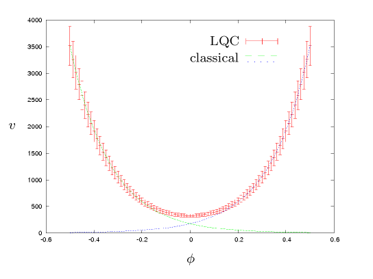
Figure 1: Expectation values and dispersions of $\hat{v}|_{\phi}$ (in red, vertical bars) in the superselection sector with $\varepsilon=1$, corresponding to the physical profile given in equation (3.14) with $\langle\hat{P}_{\phi}\rangle=1000$ and ${\Delta\hat{P}_{\phi}}/{\langle\hat{P}_{\phi}\rangle}=0.1$. The quantum evolution is also compared with the classical trajectories, one in expansion (blue curve, increasing from left to right) and the other in contraction (green curve, decreasing). Graph by courtesy of J. Olmedo.

3.7 FRW models with curvature or cosmological constant

In the previous sections, we ignored the contribution both of the intrinsic curvature $\Gamma_{a}^{i}=(\textsc{k}/2)\delta_{a}^{i}$ and of a cosmological constant $\Lambda$. Here, we sketch scenarios where the universe is not flat ($\textsc{k}=\pm 1$) and/or $\Lambda\neq 0$. For more details, consult [24].

3.7.1 Closed universe

The case of a universe with positive-definite spin connection, $\textsc{k}=1$, was studied in [22, 70, 71, 133, 158, 177, 179, 183]. Due to the extra term in the connection, the form of the classical Hamiltonian constraint (3.2) as a function of $c$ (related to metric variables as $c=\gamma\dot{a}+\textsc{k}$, a dot denotes derivative with respect to synchronous time) is modified by the replacement $c^{2}\to c(c-V_{o}^{1/3})+(1+\gamma^{2})V_{o}^{2/3}/4$. In the classical Friedmann equation, this replacement corresponds to $H^{2}\to H^{2}+\textsc{k}/a^{2}$ with $\textsc{k}=1$, where $H:=\dot{a}/a$ is the Hubble parameter. The quantum constraint and the resulting difference equation are modified accordingly. There is no arbitrariness in the fiducial volume $V_{o}$, since it can be identified with the total volume of the universe, which is finite and well defined. Then, the choice of elementary holonomy is more natural than in the flat case and, locally, one can distinguish between the group structure of $SU(2)$ and $SO(3)$ [183]. As in the flat case, the constraint operator is essentially self-adjoint [183] and the singularity at $v=0$ is removed from the quantum evolution [22, 71, 183]. However, instead of a single-bounce event one now has a cyclic model [22]. This can be traced back to the fact that the classical and quantum scalar constraint have both contracting and expanding branches coexisting in closed-universe solutions, while these branches correspond to distinct solutions in the flat case.

3.7.2 Open universe

Loop quantum cosmology of an open universe [179, 181, 191] is slightly more delicate to deal with. In contrast with the flat and closed cases $\textsc{k}=0,1$, the spin connection is non-diagonal, so that also the connection is non-diagonal and it has two (rather than one) dynamical components $c(t)$ and $c_{2}(t)$. The Gauss constraint fixes $c_{2}=1$ and one ends up with the same number of degrees of freedom as usual. The volume of the universe is infinite as in the flat case, and a fiducial volume must be defined. The classical Hamiltonian constraint is equation (3.2) with $c^{2}\to c^{2}-V_{o}^{2/3}\gamma^{2}$. The quantum constraint is constructed after defining a suitable holonomy loop; the bounce still takes place and the $v=0$ big-bang state factors out of the dynamics.

3.7.3 $\Lambda\neq 0$

Another generalization is to add a cosmological constant term, positive [71, 129, 158] or negative [32, 70, 126, 181]. At the level of the difference equation, these models have been studied in relation to the self-adjoint property.

For $\Lambda>0$, below a critical value $\Lambda_{*}$ (of order of the Planck energy), the Hamiltonian constraint operator admits many self-adjoint extensions, each with a discrete spectrum. Above $\Lambda_{*}$, the operator is essentially self-adjoint but there are no physically interesting states in the Hilbert space of the model [129].

For $\Lambda<0$, the scalar constraint is essentially self-adjoint and its spectrum is discrete [126] (while, we recall, for $\Lambda=0$ it is continuous and with support on the positive real line), also when $\textsc{k}=-1$ [181]. As in the $\Lambda=0$, $\textsc{k}=1$ case, the universe undergoes cycles of bounces [32].

4 Bianchi I model

The next step in extending loop quantum cosmology to more general situations consists in the consideration of (still homogeneous but) anisotropic cosmologies. The simplest anisotropic spacetime is the Bianchi I model, since it has flat spatial sections. This model has been extensively studied, owing to its simplicity and applications in cosmology. In fact, prior to the development of loop quantum cosmology, its quantization employing Ashtekar variables was already analyzed [23, 135, 136]. The first attempts of constructing a kinematical Hilbert space and the Hamiltonian constraint operator within a polymeric formalism were done in [40]. Then, soon after the quantization of the flat FRW model was completed within the improved dynamics scheme [21], the same programme was applied to Bianchi I, which we shall review now.

4.1 Classical formulation in Ashtekar–Barbero variables

For simplicity, we will consider the model in vacuo. Unlike the FRW universe, which is static in vacuo, the vacuum Bianchi I model has non-trivial dynamics. Its solutions are of Kasner type [130], with two expanding scale factors and the third in contraction, or vice versa.

Moreover, for later convenience, we will consider a spatial three-torus topology. Therefore, it will not be necessary to introduce any fiducial cell, since the model already provides a natural finite cell, that of the three-torus, described with angular coordinates $\{\theta,\sigma,\delta\}$ running from 0 to $2\pi$.

Like in the isotropic case, we fix the gauge and choose a diagonal flat co-triad ${}^{o}e_{a}^{i}=\delta_{a}^{i}$. The presence of three different directions requires three variables to describe the Ashtekar–Barbero connection and three more for the densitized triad, that is

$$A_{a}^{i}=\frac{c^{i}}{2\pi}\delta_{a}^{i},\qquad E_{i}^{a}=\frac{p_{i}}{4\pi^{2}}\delta_{i}^{a}\sqrt{{}^{o}q},\qquad i=\theta,\sigma,\delta.$$

The Poisson brackets defining the phase space are then $\{c^{i},p_{j}\}=8\pi G\gamma\delta^{i}_{j}$. The spacetime metric in these variables reads

$$ds^{2}=-N^{2}dt^{2}+\frac{|p_{\theta}p_{\sigma}p_{\delta}|}{4\pi^{2}}\left(\frac{d\theta^{2}}{p_{\theta}^{2}}+\frac{d\sigma^{2}}{p_{\sigma}^{2}}+\frac{d\delta^{2}}{p_{\delta}^{2}}\right).$$

In turn, the phase space is constrained by the Hamiltonian constraint

$$C_{\text{BI}}=-\frac{2}{\gamma^{2}}\frac{c^{\theta}p_{\theta}c^{\sigma}p_{\sigma}+c^{\theta}p_{\theta}c^{\delta}p_{\delta}+c^{\sigma}p_{\sigma}c^{\delta}p_{\delta}}{V}=0.$$ (4.1)

In this expression, $V=\sqrt{|p_{\theta}p_{\sigma}p_{\delta}|}$ is the physical volume of the universe.

4.2 Quantum representation

In order to polymerically represent this system, we follow the approach described in Section 3.2 [85]. Holonomies $h_{i}^{\mu_{i}}(c^{i})=e^{\mu_{i}c^{i}\tau_{i}}$ are defined along straight edges of fiducial length $2\pi\mu_{i}\in\mathbb{R}$ and oriented in the fiducial directions, here labeled by $i=\theta,\sigma,\delta$. The fluxes of the densitized triad through rectangular surfaces of fiducial area $A_{\square}^{i}$ and orthogonal to the $i$-th direction, given by $E(A_{\square}^{i},f=1)=[p_{i}/(4\pi^{2})]A_{\square}^{i}$, complete the description of the phase space before quantization. The configuration algebra is the tensor product of the algebras of quasi-periodic functions of the connection for each fiducial direction: $\text{Cyl}_{\text{S}}=\otimes_{i}\text{Cyl}_{\text{S}}^{i}=\text{lin}\{|\mu_{\theta},\mu_{\sigma},\mu_{\delta}\rangle\}$, where the kets $|\mu_{i}\rangle$ denote the quantum states corresponding to the matrix elements of the holonomies $\mathcal{N}_{\mu_{i}}(c^{i})=e^{i\mu_{i}c^{i}/2}$ in momentum representation. Hence, the kinematical Hilbert space is the tensor product $\mathcal{H}_{\text{grav}}=\otimes_{i}\mathcal{H}_{\text{grav}}^{i}$, where $\mathcal{H}_{\text{grav}}^{i}$ is the Cauchy completion of $\text{Cyl}_{\text{S}}^{i}$ with respect to the discrete inner product $\langle\mu_{i}|\mu_{i}^{\prime}\rangle=\delta_{\mu_{i}\mu_{i}^{\prime}}$.

The basic operators are $\hat{p}_{i}$ and $\hat{\mathcal{N}}_{\mu_{i}^{\prime}}$. Their action on the basis states $|\mu_{i}\rangle$ is

$$\hat{p}_{i}|\mu_{i}\rangle=p_{i}(\mu_{i})|\mu_{i}\rangle,\qquad p_{i}(\mu_{i})=4\pi\gamma l_{\text{Pl}}^{2}\mu_{i},\qquad\hat{\mathcal{N}}_{\mu_{i}^{\prime}}|\mu_{i}\rangle=|\mu_{i}+\mu_{i}^{\prime}\rangle,$$

such that $[\hat{\mathcal{N}}_{\mu_{i}},\hat{p}_{j}]=i\hbar\widehat{\{\mathcal{N}_{\mu_{i}}(c^{i}),p_{j}\}}$.

4.3 Improved dynamics

The most involved aspect that one encounters when trying to adapt the quantization of the isotropic case to the anisotropic case lies in the implementation of the improved dynamics, explained in Section 3.3. In the presence of anisotropies, we need to introduce three minimum fiducial lengths $\bar{\mu}_{i}$, when defining the curvature tensor in terms of a loop of holonomies.

Originally, a naive Ansatz was chosen, given by

$${\frac{1}{\bar{\mu}_{i}^{\prime}}}=\frac{\sqrt{|p_{i}|}}{\sqrt{\Delta}}.$$ (4.2)

This is the simplest generalization of the ansatz of the isotropic case, equation (3.5). As a consequence, the operators entering the Hamiltonian constraint have the same form as those of the flat FRW model. Furthermore, operators corresponding to different directions commute among one another. This allows to complete the quantization obtaining the physical Hilbert space [145], in the same way as for the FRW model. However, when the topology is non-compact and then a finite fiducial cell is introduced, the physical results depend on this fiducial choice [182]. This drawback led to the revision of the definition of $\bar{\mu}_{i}$, and another Ansatz free of these problems was proposed, this time given by

$${\frac{1}{\bar{\mu}_{i}}}=\frac{1}{\sqrt{\Delta}}\sqrt{\left|\frac{p_{j}p_{k}}{p_{i}}\right|}.$$ (4.3)

This choice is geometrically better justified (for a discussion about its derivation see [25]). Furthermore, this prescription is the only one verifying a remarkable property: For all the fiducial directions, the exponents $\bar{\mu}_{i}c^{i}$ of the matrix elements $\mathcal{N}_{\bar{\mu}_{i}}(c^{i})$ have a constant and fixed (up to a sign) Poisson bracket with the variable

$$v=\text{sgn}(p_{\theta}p_{\sigma}p_{\delta})\frac{\sqrt{|p_{\theta}p_{\sigma}p_{\delta}|}}{2\pi\gamma l_{\text{Pl}}^{2}\sqrt{\Delta}},$$ (4.4)

which is proportional to the volume. Note that it coincides with the parameter $v(p)$ of the isotropic case if we identify the three fiducial directions. As a consequence, as we will see, the volume will suffer constant shifts in the quantum theory, as in the isotropic case. Thanks to this property, the improved dynamics prescription (4.3) nicely implements the interplay between the anisotropies and the volume. Instead, within the naive prescription given by equation (4.2), there is no interplay between the degrees of freedom associated with different directions, because of the commutation between the operators acting on different fiducial directions. Thus, apart from giving dependencies on fiducial choices, it also seems less physically motivated.

Because of these reasons, today it is generally accepted that the more correct improved dynamics prescription is equation (4.3), which we shall consider in this paper.

4.4 Hamiltonian constraint operator

As in the isotropic case, in order to obtain the Hamiltonian constraint operator we cannot represent directly its classical form (4.1), but its expression in terms of the curvature tensor. For homogeneous models with vanishing spin connection, as Bianchi I, this expression was given in equation (3.1).

For simplicity, we will densitize the Hamiltonian constraint classically, by simply multiplying it by the volume $V$. In this way we avoid the appearance of inverse powers of the volume that make the quantum theory complicated. In any case, as seen in the flat FRW model, the densitization could be carried out with no problem in the quantum theory.

In analogy with the isotropic case, but now taking into consideration that the three fiducial directions are different, the curvature operator is the quantum counterpart of the classical expression

$${F}^{i}_{ab}=-2\sum_{j,k}\text{tr}\left(\frac{h^{\bar{\mu}}_{\square_{jk}}-\delta_{jk}}{4\pi^{2}\bar{\mu}_{j}\bar{\mu}_{k}}\tau^{i}\right)\delta^{j}_{a}\delta^{k}_{b},\qquad h^{\bar{\mu}}_{\square_{jk}}=h_{j}^{\bar{\mu}_{j}}h_{k}^{\bar{\mu}_{k}}(h_{j}^{\bar{\mu}_{j}})^{-1}(h_{k}^{\bar{\mu}_{k}})^{-1}.$$ (4.5)

Taking into account equation (4.5), the expression of the densitized triad and the definition of $\bar{\mu}_{i}$, the densitized Hamiltonian constraint for the Bianchi I model reads

$$C_{\text{BI}}=\frac{2}{\gamma^{2}\Delta}V^{2}\sum_{i,j,k}\epsilon^{ijk}\text{sgn}(p_{j})\,\text{sgn}(p_{k})\,\text{tr}\big{(}\tau_{i}h^{\bar{\mu}}_{\square_{jk}}\big{)}.$$ (4.6)

In order to represent this constraint as an operator, we first need to define the operators $\hat{\mathcal{N}}_{\bar{\mu}_{i}}$, which represent the matrix elements of the holonomies $h_{i}^{\bar{\mu}_{i}}$. To define them we follow a similar strategy to that adopted in the isotropic case. We start by reparametrizing $p_{i}(\mu_{i})$ with a parameter $\lambda_{i}(p_{i})$ such that the vectorial field $\bar{\mu}_{i}\partial_{\mu_{i}}$ produces constant translations in $\lambda_{i}$. The solution is $\lambda_{i}(p_{i})={\text{sgn}(p_{i})\sqrt{|p_{i}|}}/{(4\pi\gamma l_{\text{Pl}}^{2}\sqrt{\Delta})^{1/3}}$ [25]. The difference with respect to the isotropic case is that the translations produced by $\bar{\mu}_{i}\partial_{\mu_{i}}$, being constant with respect to the dependence on $\lambda_{i}$, do depend on the parameters $\lambda_{j}$ and $\lambda_{k}$ associated with the other two directions. In fact, we have $\bar{\mu}_{i}\partial_{\mu_{i}}=(2|\lambda_{j}\lambda_{k}|)^{-1}\partial_{\lambda_{i}}$.

As in the isotropic case, we define the operator $\hat{\mathcal{N}}_{\bar{\mu}_{i}}$ such that its action on the basis states $|\lambda_{i}\rangle$ is the same as the transformation generated by $\bar{\mu}_{i}\partial_{\mu_{i}}$ on the parameter $\lambda_{i}$, that is

$$\hat{\mathcal{N}}_{\pm\bar{\mu}_{\theta}}|\lambda_{\theta},\lambda_{\sigma},\lambda_{\delta}\rangle=\bigg{|}\lambda_{\theta}\pm\frac{1}{2|\lambda_{\sigma}\lambda_{\delta}|},\lambda_{\sigma},\lambda_{\delta}\bigg{\rangle},$$

and similarly for $\hat{\mathcal{N}}_{\pm\bar{\mu}_{\sigma}}$ and $\hat{\mathcal{N}}_{\pm\bar{\mu}_{\delta}}$. Moreover, inverting the change of variable, we obtain

$$\hat{p}_{i}|\lambda_{\theta},\lambda_{\sigma},\lambda_{\delta}\rangle=(4\pi\gamma l_{\text{Pl}}^{2}\sqrt{\Delta})^{2/3}\text{sgn}(\lambda_{i})\lambda_{i}^{2}|\lambda_{\theta},\lambda_{\sigma},\lambda_{\delta}\rangle.$$

As explained in the flat FRW case, one can always choose a suitable factor ordering for the Hamiltonian constraint that allows to remove the kernel of the volume operator, generated by the states with $\lambda_{\theta}\lambda_{\sigma}\lambda_{\delta}=0$. This is what we will consider. Therefore, the operators $\hat{\mathcal{N}}_{\bar{\mu}_{i}}$ are well defined.

The action of $\hat{\mathcal{N}}_{\pm\bar{\mu}_{i}}$ can be slightly simplified by introducing the variable $v$ defined in equation (4.4), that in terms of $\lambda$’s is given by $v=2\lambda_{\theta}\lambda_{\sigma}\lambda_{\delta}$. Indeed, making the change from, e.g., the states $|\lambda_{\theta},\lambda_{\sigma},\lambda_{\delta}\rangle$ to the states $|v,\lambda_{\sigma},\lambda_{\delta}\rangle$, one can check that, under the action of $\hat{\mathcal{N}}_{\bar{\mu}_{i}}$, $v$ suffers a constant shift equal to $1$ or $-1$ depending on the orientation of the densitized triad coefficients. On the other hand, the variables $\lambda_{\sigma}$ and $\lambda_{\delta}$ suffer a dilatation or contraction that only depends on their own sign and on $v$ (see [25] for the details).

The variable $v$ is proportional to the volume

$$\hat{V}=\widehat{\sqrt{|p_{\theta}p_{\sigma}p_{\delta}|}},\qquad\hat{V}|v,\lambda_{\sigma},\lambda_{\delta}\rangle=2\pi\gamma l_{\text{Pl}}^{2}\sqrt{\Delta}|v||v,\lambda_{\sigma},\lambda_{\delta}\rangle.$$

Therefore, as happened in the isotropic case, in this scheme the volume undergoes constant translations. The other two variables measure the degree of anisotropy of the system.

Once we know how to represent the matrix elements of the holonomies, we can promote the Hamiltonian constraint to an operator. When symmetrizing it, we will adopt the prescription of [104], whose factor ordering is analog to that considered in Section 3 (see equation (3.10)). Explicitly, it is given by [104, 147]

$$\widehat{C}_{\text{BI}}=-\frac{1}{\gamma^{2}}(\widehat{\Omega}_{\theta}\widehat{\Omega}_{\sigma}+\widehat{\Omega}_{\sigma}\widehat{\Omega}_{\theta}+\widehat{\Omega}_{\theta}\widehat{\Omega}_{\delta}+\widehat{\Omega}_{\delta}\widehat{\Omega}_{\theta}+\widehat{\Omega}_{\sigma}\widehat{\Omega}_{\delta}+\widehat{\Omega}_{\delta}\widehat{\Omega}_{\sigma}),$$ (4.7)

where

$$\widehat{\Omega}_{i}=\frac{1}{4i\sqrt{\Delta}}\widehat{\sqrt{V}}\left[\big{(}\hat{\mathcal{N}}_{2\bar{\mu}_{i}}-\hat{\mathcal{N}}_{-2\bar{\mu}_{i}}\big{)}\widehat{\text{sgn}(p_{i})}+\widehat{\text{sgn}(p_{i})}\big{(}\hat{\mathcal{N}}_{2\bar{\mu}_{i}}-\hat{\mathcal{N}}_{-2\bar{\mu}_{i}}\big{)}\right]\widehat{\sqrt{V}}.$$ (4.8)

This operator differs from that of [25] in the treatment applied to the signs of $p_{i}$ when symmetrizing. Then, $\widehat{{C}}_{\text{BI}}$ not only decouples the zero-volume states, but also it does not relate states with opposite orientation of any of the triad coefficients, namely, states $|v,\lambda_{\sigma},\lambda_{\delta}\rangle$ with opposite sign in any of their quantum numbers. Therefore, $\widehat{{C}}_{\text{BI}}$ leaves invariant all the octants in the tridimensional space defined by $v$, $\lambda_{\sigma}$ and $\lambda_{\delta}$. Hence, we can restrict the study to any of them. We will restrict ourselves to the subspace of positive densitized triad coefficients, given by

$${\text{Cyl}}_{\text{S}}^{+}=\text{lin}\{|v,\lambda_{\sigma},\lambda_{\delta}\rangle;\,v,\lambda_{\sigma},\lambda_{\delta}>0\}.$$

The action of $\widehat{{C}}_{\text{BI}}$ on the states of ${\text{Cyl}}_{\text{S}}^{+}$ turns out to be

$$\widehat{{C}}_{\text{BI}}|v,\lambda_{\sigma},\lambda_{\delta}\rangle=\frac{(\pi l_{\text{Pl}}^{2})^{2}}{4}\big{[}x_{-}(v)|v-4,\lambda_{\sigma},\lambda_{\delta}\rangle_{-}-x^{-}_{0}(v)|v,\lambda_{\sigma},\lambda_{\delta}\rangle_{-}$$

$$\phantom{\widehat{{C}}_{\text{BI}}|v,\lambda_{\sigma},\lambda_{\delta}\rangle=}{}-x^{+}_{0}(v)|v,\lambda_{\sigma},\lambda_{\delta}\rangle_{+}+x_{+}(v)|v+4,\lambda_{\sigma},\lambda_{\delta}\rangle_{+}\big{]},$$

where we have introduced the coefficients

$$x_{-}(v)=2\sqrt{v}(v-2)\sqrt{v-4}[1+\text{sgn}(v-4)],\qquad x_{+}(v)=x_{-}(v+4),$$ (4.9a)

$$x^{-}_{0}(v)=2(v-2)v[1+\text{sgn}(v-2)],\qquad x^{+}_{0}(v)=x^{-}_{0}(v+2),$$ (4.9b)

and the following linear combination of states

$$|v\pm n,\lambda_{\sigma},\lambda_{\delta}\rangle_{\pm}=\bigg{|}v\pm n,\lambda_{\sigma},\frac{v\pm n}{v\pm 2}\lambda_{\delta}\bigg{\rangle}+\bigg{|}v\pm n,\frac{v\pm n}{v\pm 2}\lambda_{\sigma},\lambda_{\delta}\bigg{\rangle}$$

$$\hphantom{|v\pm n,\lambda_{\sigma},\lambda_{\delta}\rangle_{\pm}=}{}+\bigg{|}v\pm n,\frac{v\pm 2}{v}\lambda_{\sigma},\lambda_{\delta}\bigg{\rangle}+\bigg{|}v\pm n,\lambda_{\sigma},\frac{v\pm 2}{v}\lambda_{\delta}\bigg{\rangle}$$

$$\hphantom{|v\pm n,\lambda_{\sigma},\lambda_{\delta}\rangle_{\pm}=}{}+\bigg{|}v\pm n,\frac{v\pm 2}{v}\lambda_{\sigma},\frac{v\pm n}{v\pm 2}\lambda_{\delta}\bigg{\rangle}+\bigg{|}v\pm n,\frac{v\pm n}{v\pm 2}\lambda_{\sigma},\frac{v\pm 2}{v}\lambda_{\delta}\bigg{\rangle}.$$ (4.10)

Note that, in fact, the operator $\widehat{{C}}_{\text{BI}}$ is well defined in ${\text{Cyl}}_{\text{S}}^{+}$, since $x_{-}(v)=0$ if $v\leq 4$, and $x^{-}_{0}(v)=0$ if $v\leq 2$. Since there is no $v=0$ state, the singularity has no longer analog in the kinematical Hilbert space, and then is resolved already kinematically.

4.5 Superselection sectors

The analysis of the action of $\widehat{C}_{\text{BI}}$ on a generic basis state $|v,\lambda_{\sigma}^{\star},\lambda_{\delta}^{\star}\rangle$ shows that:

• Concerning the variable $v$, it suffers a constant shift equal to $4$ or $-4$, the latest only if $v>4$. Therefore, $\widehat{{C}}_{\text{BI}}$ preserves the subspace of states whose quantum number $v$ belongs to any of the semilattices of step four

  $$\mathcal{L}_{\varepsilon}^{+}=\{\varepsilon+4k,k=0,1,2,\dots\},\qquad\varepsilon\in(0,4].$$

• Concerning the anisotropy variables, $\lambda_{\sigma}$ and $\lambda_{\delta}$, the effect upon them does not depend on the initial quantum numbers $\lambda_{\sigma}^{\star}$ and $\lambda_{\delta}^{\star}$, but only on $v=\varepsilon+4k$. Moreover, this dependence occurs via fractions whose denominator is two units bigger or smaller than the numerator. As a consequence, the iterative action of the constraint operator on $|v,\lambda_{\sigma}^{\star},\lambda_{\delta}^{\star}\rangle$, only relates this state with states whose quantum numbers $\lambda_{\sigma}$ and $\lambda_{\delta}$ are of the form $\lambda_{a}=\omega_{\varepsilon}\lambda_{a}^{\star}$, with $\omega_{\varepsilon}$ belonging to the set

  $$\mathcal{W}_{\varepsilon}=\bigg{\{}\left(\frac{\varepsilon-2}{\varepsilon}\right)^{z}\prod_{m,n\in\mathbb{N}}\left(\frac{\varepsilon+2m}{\varepsilon+2n}\right)^{k_{n}^{m}};$$

  $$\hphantom{W_{\varepsilon}=\bigg{\{}}{}k_{n}^{m}\in\mathbb{N},\;z\in\mathbb{Z}\text{ if }\varepsilon>2,\;\;z=0\text{ if }\varepsilon<2\bigg{\}}.$$ (4.11)

The set $\mathcal{W}_{\varepsilon}$ is infinite and, moreover, one can prove that it is dense in the positive real line [104]. Nonetheless, it is countable. Therefore, while the variable $v$ has support in simple semilattices of constant step, the variables $\lambda_{a}$ take values belonging to complicated sets, but they also provide separable subspaces. As a concrete example, we see that, if both $\varepsilon$ and $\lambda_{a}^{\star}$ are integers, then $\lambda_{a}$ take values in the positive rational numbers.

In conclusion, the operator $\widehat{{C}}_{\text{BI}}$ leaves invariant the Hilbert subspaces $\mathcal{H}^{+}_{\varepsilon,\lambda_{\sigma}^{\star},\lambda_{\delta}^{\star}}$, defined as the Cauchy completion of

$$\text{Cyl}^{+}_{\varepsilon,\lambda_{\sigma}^{\star},\lambda_{\delta}^{\star}}=\text{lin}\big{\{}|v,\lambda_{\sigma},\lambda_{\delta}\rangle;\;v\in\mathcal{L}_{\varepsilon}^{+},\;\lambda_{a}=\omega_{\varepsilon}\lambda_{a}^{\star},\;\omega_{\varepsilon}\in\mathcal{W}_{\varepsilon},\;\lambda_{a}^{\star}\in\mathbb{R}^{+}\big{\}},$$

with respect to the discrete inner product $\langle v,\lambda_{\sigma},\lambda_{\delta}|v^{\prime},\lambda^{\prime}_{\sigma},\lambda^{\prime}_{\delta}\rangle=\delta_{vv^{\prime}}\delta_{\lambda_{\sigma}\lambda^{\prime}_{\sigma}}\delta_{\lambda_{\delta}\lambda^{\prime}_{\delta}}$. As we will see, physical observables also preserve these separable subspaces $\mathcal{H}^{+}_{\varepsilon,\lambda_{\sigma}^{\star},\lambda_{\delta}^{\star}}$, and therefore they provide sectors of superselection, and we can restrict the study to any of them.

4.6 Physical Hilbert space

The Hamiltonian constraint operator $\widehat{{C}}_{\text{BI}}$ is quite complicated and, unlike the isotropic case (and unlike previous quantizations of the model [145]), its spectral properties have not been determined. Consequently, it has not been diagonalized either. Therefore, the group averaging approach is not useful in this situation, and to analyze the physical solutions one has to impose the constraint directly on the dual space $(\text{Cyl}^{+}_{\varepsilon,\lambda_{\sigma}^{\star},\lambda_{\delta}^{\star}})^{*}$. The elements $(\psi|$ of that space have the formal expansion

$$(\psi|=\sum_{v\in\mathcal{L}_{\varepsilon}^{+}}\sum_{\omega_{\varepsilon}\in\mathcal{W}_{\varepsilon}}\sum_{\bar{\omega}_{\varepsilon}\in\mathcal{W}_{\varepsilon}}\psi(v,\omega_{\varepsilon}\lambda_{\sigma}^{\star},\bar{\omega}_{\varepsilon}\lambda_{\delta}^{\star})\big{\langle}v,\omega_{\varepsilon}\lambda_{\sigma}^{\star},\bar{\omega}_{\varepsilon}\lambda_{\delta}^{\star}\big{|}.$$

From the action of $\widehat{C}_{\text{BI}}$, one obtain that the constraint $\big{(}\psi\big{|}\widehat{\mathcal{C}}_{\text{BI}}^{\text{B}}{}^{\dagger}=0$ leads to the following recurrence relation,

$$\psi_{+}(v+4,\lambda_{\sigma},\lambda_{\delta})=\frac{1}{x_{+}(v)}\big{[}{x^{-}_{0}(v)}\psi_{-}(v,\lambda_{\sigma},\lambda_{\delta})+{x^{+}_{0}(v)}\psi_{+}(v,\lambda_{\sigma},\lambda_{\delta})$$

$$\hphantom{\psi_{+}(v+4,\lambda_{\sigma},\lambda_{\delta})=\frac{1}{x_{+}(v)}\big{[}}{}-{x_{-}(v)}\psi_{-}(v-4,\lambda_{\sigma},\lambda_{\delta})\big{]}.$$

In this expression, in order to simplify the notation, we have introduced the projections of $(\psi|$ on the linear combinations of six states defined in equation (4.10), namely,

$$\psi_{\pm}(v\pm n,\lambda_{\sigma},\lambda_{\delta})=(\psi|v\pm n,\lambda_{\sigma},\lambda_{\delta}\rangle_{\pm}.$$

Owing to the property $x_{-}(\varepsilon)=0$, the above recurrence relation, that is of order 2 in the variable $v$, becomes a first-order equation if $v=\varepsilon$:

$$\psi_{+}(\varepsilon+4,\lambda_{\sigma},\lambda_{\delta})=\frac{1}{x_{+}(\varepsilon)}\big{[}{x^{-}_{0}(\varepsilon)}\psi_{-}(\varepsilon,\lambda_{\sigma},\lambda_{\delta})+{x^{+}_{0}(\varepsilon)}\psi_{+}(\varepsilon,\lambda_{\sigma},\lambda_{\delta})\big{]}.$$

Therefore, if we know all the data in the initial section $v=\varepsilon$, we obtain all the combinations of six terms given by

$$\psi_{+}(\varepsilon+4,\lambda_{\sigma},\lambda_{\delta})=\psi\left(\varepsilon+4,\lambda_{\sigma},\frac{\varepsilon+4}{\varepsilon+2}\lambda_{\delta}\right)+\psi\left(\varepsilon+4,\frac{\varepsilon+4}{\varepsilon+2}\lambda_{\sigma},\lambda_{\delta}\right)$$

$$\hphantom{\psi_{+}(\varepsilon+4,\lambda_{\sigma},\lambda_{\delta})=}{}+\psi\left(\varepsilon+4,\lambda_{\sigma},\frac{\varepsilon+2}{\varepsilon}\lambda_{\delta}\right)+\psi\left(\varepsilon+4,\frac{\varepsilon+2}{\varepsilon}\lambda_{\sigma},\lambda_{\delta}\right)$$

$$\hphantom{\psi_{+}(\varepsilon+4,\lambda_{\sigma},\lambda_{\delta})=}{}+\psi\left(\varepsilon+4,\frac{\varepsilon+2}{\varepsilon}\lambda_{\sigma},\frac{\varepsilon+4}{\varepsilon+2}\lambda_{\delta}\right)+\psi\left(\varepsilon+4,\frac{\varepsilon+4}{\varepsilon+2}\lambda_{\sigma},\frac{\varepsilon+2}{\varepsilon}\lambda_{\delta}\right).$$

From the combinations $\psi_{+}(\varepsilon+4,\lambda_{\sigma},\lambda_{\delta})$, it is possible to determine any of the individual terms $\psi(\varepsilon+4,\lambda_{\sigma},\lambda_{\delta})$ that compose them, since it has been shown that the system of equations that relate the formers with the latters is formally invertible [147]. This has been proven not only for $v=\varepsilon+4$ but also for all $v\in\mathcal{L}_{\varepsilon}^{+}$. In conclusion, the physical solutions of the Hamiltonian constraint are completely determined by the set of initial data

$$\{\psi(\varepsilon,\lambda_{\sigma},\lambda_{\delta})=\psi(\varepsilon,\omega_{\varepsilon}\lambda_{\sigma}^{\star},\bar{\omega}_{\varepsilon}\lambda_{\delta}^{\star}),\ \omega_{\varepsilon},\bar{\omega}_{\varepsilon}\in\mathcal{W}_{\varepsilon},\ \lambda_{\sigma}^{\star},\lambda_{\delta}^{\star}\in\mathbb{R}^{+}\},$$

and we can identify solutions with this set. We can also characterize the physical Hilbert space as the Hilbert space of the initial data. In order to endow the set of initial data with a Hilbert structure, one can take a complete set of observables forming a closed algebra, and impose that the quantum counterpart of their complex conjugation relations become adjointness relations between operators. This determines a unique (up to unitary equivalence) inner product.

Before doing that, it is suitable to change the notation. Following [147], let us introduce the variables $x_{a}=\ln(\lambda_{a})=\ln(\lambda_{a}^{\star})+\rho_{\varepsilon}$. Note that $\rho_{\varepsilon}$ takes values in a dense set of the real line, given by the logarithm of the points in the set $\mathcal{W}_{\varepsilon}$. We will denote that set by $\mathcal{Z}_{\varepsilon}$. For each direction $a=\sigma$ or $\delta$, we consider the linear span $\text{Cyl}_{\lambda_{a}^{\star}}$ of the states whose support is just one point $x_{a}$ of the superselection sector defined by taking the product of $\lambda_{a}^{\star}$ with all the points in the set $\mathcal{Z}_{\varepsilon}$. We call $\mathcal{H}_{\lambda_{a}^{\star}}$ the Hilbert completion of this vector space with the discrete inner product.

Then, a set of observables acting on the initial data $\tilde{\psi}(x_{\sigma},x_{\delta}):=\psi(\varepsilon,x_{\sigma},x_{\delta})$ is that formed by the operators $\widehat{e^{ix_{a}}}$ and $\widehat{U}_{a}^{\rho_{a}}$, with $\rho_{a}\in\mathcal{Z}_{\varepsilon}$ and $a=\sigma,\delta$, defined as

$$\widehat{e^{ix_{\sigma}}}\tilde{\psi}(x_{\sigma},x_{\delta})={e^{ix_{\sigma}}}\tilde{\psi}(x_{\sigma},x_{\delta}),\qquad\widehat{U}_{\sigma}^{\rho_{\sigma}}\tilde{\psi}(x_{\sigma},x_{\delta})=\tilde{\psi}(x_{\sigma}+\rho_{\sigma},x_{\delta}),$$ (4.12)

and similarly for $\widehat{e^{ix_{\delta}}}$ and $\widehat{U}_{\delta}^{\rho_{\delta}}$. These operators provide an overcomplete set of observables and are unitary in $\mathcal{H}_{\lambda_{\sigma}^{\star}}\otimes\mathcal{H}_{\lambda_{\delta}^{\star}}$, according with their reality conditions. Therefore, we conclude that this Hilbert space is precisely the physical Hilbert space of the vacuum Bianchi I model.

Owing to the complicated form of the solutions, together with the fact that a basis of eigenfunctions of the Hamiltonian constraint operator is not known, the evolution picture of this model has not been studied yet. It is expected that, as in the isotropic models, a quantum bounce solves dynamically the big bang singularity. Indeed, this has been already checked using an effective dynamics [84], in the case of the model coupled to a massless scalar field, as in the FRW case. In this respect, it is worth commenting that in analyses where a massless scalar field is introduced, the latter serves as internal time to describe the notion of evolution, as seen in Section 3.5.2. This field (unlike the geometric degrees of freedom) is quantized adopting a standard Schrödinger-like representation, which makes straightforward the construction of a family of unitarily related observables parametrized by the internal time. However, in vacuum cases such as the Bianchi I model we have just described, where a suitable matter field is not at hand, it would be interesting to describe the evolution regarding as internal time one of the geometry degrees of freedom. There is a complication because of the fact that such internal time is polymeric, since the geometry degrees of freedom are polymerically quantized. Although such description has not been carried out for the Bianchi I model within the current improved dynamics, it has been nonetheless constructed for the vacuum Bianchi I model quantized within the naive improved dynamics given in equation (4.2). That was done in [146], and an analog construction could just as well serve to describe the evolution of the current vacuum Bianchi I model (quantized within the scheme given in equation (4.3)), using either the volume variable $v$ or its momentum as internal time.

4.7 Loop quantization of other Bianchi models

Bianchi models are characterized by possessing three spatial Killing fields. In the case of the Bianchi I model, the Killing fields commute and, then, it is the simplest of the Bianchi models. This is the reason why it has been extensively studied in the literature, and in particular in the framework of LQC. Nevertheless, loop quantization has been also extended to other Bianchi models (with non-commuting Killing fields), in particular to Bianchi II and Bianchi IX. A preliminary loop quantization of these models was already considered just after the birth of LQC [40, 59]. More recently, their quantization has been achieved implementing the improved dynamics developed for Bianchi I, in [26] for Bianchi II and in [201] for Bianchi IX. In the following we summarize the main characteristics of these works. We refer the reader to those references for further details.

Both the Bianchi II and the Bianchi IX models possess non-commuting Killing fields. As a consequence, the fiducial triad and co-triad cannot be chosen to be diagonal, a first feature that complicates the analysis in comparison with Bianchi I. Moreover, the spin connection of those models is non-trivial. After choosing a suitable gauge and appropriate parameterizations for the Ashtekar–Barbero variables, the Hamiltonian constraint of both Bianchi II and Bianchi IX consists in that of the (analog) Bianchi I model plus an extra term, of course different for each model, but that in both cases involves components of the connection and inverses of the densitized triad coefficients.

The kinematical Hilbert space of the Bianchi II and IX models is identical to that of Bianchi I. The main difficulty lies in the representation of the components of the connection that appear in the extra term of the Hamiltonian constraint. To tackle this issue, the strategy adopted is to define an operator representing the connection [26, 202], choosing a suitable loop of holonomies and implementing the ideas employed when constructing the curvature operator for Bianchi I. As a result, the components $c^{i}$ of the connection turn out to be represented by the polymeric operator

$$\hat{c}_{i}=\widehat{\frac{\sin\bar{\mu}_{i}c^{i}}{\bar{\mu}_{i}}},$$

where $\bar{\mu}_{i}$ is the minimum length defined in equation (4.3).

Once the above operator is defined, the representation of the Hamiltonian constraint as a symmetric operator follows straightforwardly, in the same way as for the Bianchi I model. Once again, classical singularities are avoided in both models, since the kernel of the volume operator can be removed from their quantum theories.

Part II Midisuperspace models in loop quantum gravity

In the previous part we have discussed the loop quantization of several homogeneous cosmological models. In all of them the classical cosmological singularity is avoided. Nonetheless, it is natural to ask whether the resolution of the singularity is an intrinsic feature of the loop quantization or, on the contrary, if it is a result due to the high symmetry of the homogeneous models. In order to answer this question, it seems inevitable to extend the loop quantization to inhomogeneous systems. Furthermore, it is essential to make this step in order to develop a realistic theory of quantum cosmology. Indeed, as the results obtained in modern cosmology indicate, in the early universe the inhomogeneities played a fundamental role in the formation of the cosmic structures that we observe today.

The quantization of inhomogeneous models is technically more complicated than that of minisuperspaces, since they possess field degrees of freedom, as the full theory. Hopefully, facing the loop quantization of midisuperspaces we will get insights about the open problems present in loop quantum gravity.

In this section we will review the status of loop quantization of midisuperspace models. Classically, these models have Killing vectors which reduce the degrees of freedom of the metric but the number of Killing vectors are low enough to ensure that the remaining degrees of freedom are local. The metrics are therefore parametrized by functions of time and spatial coordinate(s). Thus, unlike minisuperspace scenarios, midisuperspace models are field theories (for a comprehensive review, see [31]). Questions beyond the reach of minisuperspace models can be addressed in the study of midisuperspaces both classically as well as in the context of a particular quantization scheme. In the context of LQG, these issues may include the construction of Dirac observables or of quasilocal observables, the closure of the quantum constraint algebra and, most importantly, whether the singularity resolution mechanism of LQC continues to be valid in the field theory context.

There exist a number of midisuperspace models but the loop quantization procedure has been attempted only in a few of them so far. One important class of models is obtained by symmetry reduction of GR.

• Spherical symmetry. In $3+1$ dimensions, a spacetime is called spherically symmetric if its isometry group contains a subgroup isomorphic to $SO(3)$, and the orbits of this subgroup are 2-spheres such that the induced metric thereon is Riemannian and proportional to the unit round metric on $S^{2}$. These are, in a sense, midway between the minisuperspace models and models with an infinite number of physical degrees of freedom. Spherically symmetric spacetime metrics depend on the radial coordinate, and therefore these models have to be treated as field theories. However, in vacuum, the physical solutions are characterized by only a single parameter according to Birkhoff’s theorem. In that respect they are dynamically trivial, although the gauge-fixing procedure is extremely non-trivial. To make them into physical field theories, we need to add matter in the form of dust shells.

  Here we are mainly interested in cosmological models while the spherical symmetric models are mostly black hole solutions, in particular the Schwarzschild solution. Hence, we will briefly mention the progress made in the context of LQG for completeness.

  In [54] the kinematical framework for studying spherically symmetric models in LQG was introduced. The volume operator was constructed in [69] and it was shown that the volume eigenstates are not eigenstates of the flux operator. Consequently, the standard prescription of constructing the Hamiltonian operator cannot be used. This problem was circumvented in [68], where the Hamiltonian constraint operator was constructed in terms of non-standard variables which mix the connection and the extrinsic curvature. This formulation was extended to explore the question of singularity resolution of Schwarzschild black holes in [51] and the Lemaître–Toleman–Bondi collapse of a spherical inhomogeneous dust cloud in [60]. The choice of variables made in the above programme is similar to the polymer quantization of the Gowdy $T^{3}$ model, which will be described in detail later. Since the basic quantum variables used in these constructions are different from the basic quantum variables of the full theory, another approach in loop quantization of the spherically symmetric models was explored in [82]. In this approach, the diffeomorphism constraint is fixed leaving the Gauss and the Hamiltonian constraints. The latter is then applied to the Schwarzschild solution. The exterior solutions agree with the ones obtained in geometrodynamics. The interior solution was studied in [83] where it was shown that, after a partial gauge fixing, it can be mapped to the minisuperspace Kantowski–Sachs model. After loop quantization, the singularity is replaced by a bounce. In [103] the issue of the residual diffeomorphism invariance of loop-quantized spherical symmetric models has been investigated. Although the quantization programme is still incomplete, the studies done so far indicate that the singularity resolution mechanism described in the previous section may be a robust feature of loop quantization.

Another class of midisuperspace models can be roughly classified on the isometry group of the metric. In most cases, this is equivalent to a classification based on the number of Killing vectors of the metric.

• Spacetimes with one Killing vector. These models are obtained by symmetry reduction corresponding to one-dimensional spatial isometry groups taken to be ${\mathbb{R}}$ or $U(1)$. Some of the important features of GR are retained, such as diffeomorphism invariance and the field-theoretic non-linear nature of the physical degrees of freedom. It was shown in [105] that, locally, it is possible to interpret these $3+1$ dimensional models as $2+1$ dimensional general relativity coupled to two matter fields, a scalar field and a one-form field corresponding, respectively, to the norm and the twist of the four-dimensional Killing vector field. However, not much work has been done so far in loop quantizing this reduced system apart from the preliminary analysis carried out in [121] in terms of complex Ashtekar variables.

• Spacetimes with two Killing vectors. The next level of simplification is to consider two-dimensional spacelike isometry groups. Two types of group action and spatial topologies have been studied in LQG:

  • Isometry group of ${\mathbb{R}}\times U(1)$ with the spatial topology being ${\mathbb{R}}^{3}$. These correspond to Einstein–Rosen cylindrical waves. An preliminary attempt has been made to construct the kinematic Hilbert space and define the volume operator (see Section 5.11 of [44]), although there has not been much progress so far.

  • Isometry group of $U(1)\times U(1)$ with the spatial topology being $T^{3}$. These correspond to Gowdy models.

  If we impose the additional condition that the Killing vectors are mutually orthogonal, we obtain polarized models. These are the simplest midisuperspace models with only one field theory degree of freedom. An example is the polarized Gowdy $T^{3}$ model. This has been studied in some detail in LQG from two different perspectives, both of which will be described in detail in the next two sections.

5 Hybrid quantization of the polarized Gowdy $T^{3}$ model

Gowdy models are among the best known inhomogeneous cosmologies [107, 108]. They represent globally hyperbolic vacuum spacetimes, with compact spatial sections and with two spatial Killing fields. The simplest example is the linearly polarized Gowdy $T^{3}$ model. Indeed, its classical solutions are exactly known [125, 161, 162]. They represent gravitational waves propagating in a closed expanding universe. Its standard quantization was already considered since the 70’s [33, 34, 35, 91, 94, 159, 164, 189]. Moreover, a Fock quantization of the model, in which the dynamics is implemented unitarily, was achieved [88, 89], and it has been shown that this quantization is essentially unique [90, 98] (in a sense that we will explain later).

In order to apply the quantization employed in LQC to this model, the simplest possibility is to carry out a hybrid quantization, that combines the polymeric quantization of the degrees of freedom that parametrize the homogeneous solutions, with the Fock quantization for the inhomogeneities. This hybrid quantization was developed in [104, 141, 151]. Here we summarize its construction and main results.

5.1 Classical description of the Gowdy $T^{3}$ model

The Gowdy $T^{3}$ model represents vacuum solutions to the Einstein equations, with two spatial Killing fields that commute, and with spatial hypersurfaces homeomorphic to a three-torus. As said before, we will consider the linearly polarized model, that possesses an additional symmetry: the Killing vectors are orthogonal to hypersurfaces and, therefore, are mutually orthogonal everywhere. Letting $\partial_{\sigma}$ and $\partial_{\delta}$ be the Killing vectors, the model admits global coordinates $\{t,\theta,\sigma,\delta\}$ adapted to the symmetries, with $\theta,\sigma,\delta\in S^{1}$.

After a 3+1 decomposition, we can describe the spacetime metric in terms of the three-metric $q_{ab}$ induced in the spatial sections foliating the four-dimensional manifold, the densitized lapse ${N_{{}_{{}_{\!\!\!\!\!\!\sim}}\;}}=N/\sqrt{q}$, and the shift vector $N^{a}$, with $a,b\in\{\theta,\sigma,\delta\}$. Owing to the isometries $\partial_{\sigma}$ and $\partial_{\delta}$, the Gowdy model verifies $q_{\theta\sigma}=0=q_{\theta\delta}$. This condition fixes the gauge freedom associated with the momentum constraint in those directions, and implies $N^{\sigma}=0=N^{\delta}$ [152]. As a consequence, the metric components only depend on $t$ and $\theta$ and are periodic in the latter. This periodicity allows us to decompose the metric components in Fourier modes. On the other hand, the condition of linear polarization imposes $q_{\sigma\delta}=0$. Therefore, the three-metric is diagonal and can be described by three fields $(\tau,\xi,\bar{\gamma})$, that essentially characterize the area of the isometry group orbits, the norm of one of the Killing vectors, and the scale factor of the metric induced on the set of group orbits. The phase space is then parametrized by those fields and by their momenta $(P_{\tau},P_{\xi},P_{\bar{\gamma}})$, and constrained by the $\theta$-momentum constraint and by the Hamiltonian constraint [88].

In order to prepare the model for its quantization, the gauge is further reduced. One imposes that the generator of the conformal transformations, $P_{\bar{\gamma}}$, and the area of the isometry group orbits, $\tau$, are homogeneous functions. These conditions fix the gauge freedom associated with the non-zero Fourier modes of the $\theta$-momentum constraint and of the densitized Hamiltonian constraint, and imply that the functions $N_{\theta}$ and ${N_{{}_{{}_{\!\!\!\!\!\!\sim}}\;}}$ are homogeneous [88, 141, 151]. Then, two global constraints remain in the model, the spatial average of the $\theta$-momentum constraint, generating rigid rotations in the circle, and the spatial average of the densitized Hamiltonian constraint. We will denote them by $C_{\theta}$ and $C_{\text{G}}$, respectively.

The classically reduced phase space can be split into homogeneous and inhomogeneous sectors. The homogeneous sector coincides with the phase space of the Bianchi I spacetime with three-torus topology. This sector will be quantized à la LQC, and therefore is parametrized by the variables $\{(c^{i},p_{i}),i=\theta,\sigma,\delta\}$, with Poisson bracket $\{c^{i},p_{j}\}=8\pi G\gamma\delta^{i}_{j}$, as described in Section 4. The inhomogeneous sector is given by the non-zero (inhomogeneous) modes of the fields unaffected by the gauge fixing, namely $\{(\xi_{{}_{m}},P_{\xi_{{}_{m}}}),m\in\mathbb{Z}\setminus\{0\}\}$. This sector will be quantized employing the Fock quantization of [88]. To employ this Fock representation, the above inhomogeneous modes are in turn described by annihilation and creation variables $(a_{m},a_{m}^{*})$, defined as those related to a free massless scalar field. This quantization is preferred as long as is the only Fock quantization of the deparametrized system in which the dynamics is unitary and with a vacuum invariant under the $S^{1}$ translations (the remaining symmetry after gauge fixing) [90, 98].

The three-metric in terms of the chosen variables reads [104]

$$ds^{2}=-q_{\theta\theta}\left(\frac{|p_{\theta}|}{4\pi^{2}}\right)^{2}{N_{{}_{{}_{\!\!\!\!\!\!\sim}}\;}}^{2}dt^{2}+q_{\theta\theta}d\theta^{2}+q_{\sigma\sigma}d\sigma^{2}+q_{\delta\delta}d\delta^{2},$$

$$q_{\theta\theta}=\frac{1}{4\pi^{2}}\left|\frac{p_{\sigma}p_{\delta}}{p_{\theta}}\right|\exp\left\{\frac{2\pi}{\sqrt{|p_{\theta}|}}\frac{c^{\delta}p_{\delta}-c^{\sigma}p_{\sigma}}{c^{\sigma}p_{\sigma}+c^{\delta}p_{\delta}}\tilde{\xi}(\theta)-\frac{\pi^{2}}{|p_{\theta}|}[\tilde{\xi}(\theta)]^{2}-\frac{8\pi G\gamma}{c^{\sigma}p_{\sigma}+c^{\delta}p_{\delta}}\zeta(\theta)\right\},$$

$$q_{\sigma\sigma}=\frac{1}{4\pi^{2}}\left|\frac{p_{\theta}p_{\delta}}{p_{\sigma}}\right|\exp\left\{-\frac{2\pi}{\sqrt{|p_{\theta}|}}\tilde{\xi}(\theta)\right\},$$

$$q_{\delta\delta}=\frac{1}{4\pi^{2}}\left|\frac{p_{\theta}p_{\sigma}}{p_{\delta}}\right|\exp\left\{\frac{2\pi}{\sqrt{|p_{\theta}|}}\tilde{\xi}(\theta)\right\},$$ (5.1)

where the inhomogeneities are encoded in the terms

$$\tilde{\xi}(\theta)=\frac{1}{\pi}\sum_{m\neq 0}\sqrt{\frac{G}{|m|}}(a_{m}+a_{-m}^{*})e^{im\theta},$$

$$\zeta(\theta)=i\sum_{m\neq 0}\sum_{\tilde{m}\neq 0}\text{sgn}(m+\tilde{m})\frac{\sqrt{|m+\tilde{m}||\tilde{m}|}}{|m|}(a_{-\tilde{m}}-a^{*}_{\tilde{m}}\big{)}\big{(}a_{m+\tilde{m}}+a^{*}_{-(m+\tilde{m})}\big{)}e^{im\theta}.$$

On the other hand, the remaining constraints have the following form:

$$C_{\theta}=\sum_{m=1}^{\infty}m(a_{m}^{*}a_{m}-a_{-m}^{*}a_{-m})=0,$$

$$C_{\text{G}}=C_{\text{BI}}+C_{\xi}=0,\quad C_{\xi}={G}\left[\frac{(c^{\sigma}p_{\sigma}+c^{\delta}p_{\delta})^{2}}{\gamma^{2}|p_{\theta}|}H_{\text{int}}^{\xi}+32\pi^{2}|p_{\theta}|H_{0}^{\xi}\right].$$ (5.2)

In the above expression,

$$H_{\text{int}}^{\xi}=\sum_{m\neq 0}\frac{1}{2|m|}\left[2a^{*}_{m}a_{m}+a_{m}a_{-m}+a^{*}_{m}a^{*}_{-m}\right],\qquad H_{0}^{\xi}=\sum_{m\neq 0}|m|a^{*}_{m}a_{m},$$ (5.3)

and $C_{\text{BI}}$ is the (densitized) Hamiltonian constraint of the Bianchi I model given in equation (4.6). In the Hamiltonian constraint, the inhomogeneities appear in the term $H_{0}^{\xi}$, that corresponds to the Hamiltonian of a free massless scalar field, and in the term $H_{\text{int}}^{\xi}$, that represents an interaction term. The inhomogeneities are coupled to the homogeneous sector in a non-trivial way, so that the feasibility of the hybrid quantization is not straightforward a priori.

5.2 Fock quantization of the inhomogeneous sector

Once the inhomogeneous sector is described with the appropriate annihilation and creation like variables, $a_{m}$ and $a^{*}_{m}$, it is straightforward to get its Fock quantization. With that aim, we promote the variables $a_{m}$ and $a^{*}_{m}$ to annihilation and creation operators, $\hat{a}_{m}$ and $\hat{a}^{\dagger}_{m}$ respectively, such that $[\hat{a}_{m},\hat{a}^{\dagger}_{\tilde{m}}]=\delta_{m\tilde{m}}$. From the vacuum state $|0\rangle$, characterized by the equations

$$\hat{a}_{m}|0\rangle=0,\qquad\forall\,m\in\mathbb{Z},$$

we construct the one-particle Hilbert space, and the associated symmetric Fock space $\mathcal{F}$ [197]. The annihilation and creation operators are densely defined in the subspace of $\mathcal{F}$ given by finite linear combinations of $n$-particle states

$$|\mathfrak{n}\rangle:=|\dots,n_{-2},n_{-1},n_{1},n_{2},\dots\rangle,$$

such that $\sum_{m}n_{m}<\infty$, being $n_{m}\in\mathbb{N}$ the occupation number (or number of particles) of the $m$-th mode. We will denote that space by $\mathcal{S}$. Note that the $n$-particle states provide a basis for the Fock space, orthonormal with respect to the inner product $\langle\mathfrak{n}^{\prime}|\mathfrak{n}\rangle=\delta_{\mathfrak{n}^{\prime}\mathfrak{n}}$. The action of $\hat{a}_{m}$ and $\hat{a}^{\dagger}_{m}$ on these states is

$$\hat{a}_{m}|\dots,n_{m},\dots\rangle=\sqrt{n_{m}}|\dots,n_{m}-1,\dots\rangle,$$

$$\hat{a}_{m}^{\dagger}|\dots,n_{m},\dots\rangle=\sqrt{n_{m}+1}|\dots,n_{m}+1,\dots\rangle.$$

5.2.1 Generator of translations in the circle

The constraint that generates translations in the circle, $C_{\theta}$, does not affect the homogeneous sector, and then it is represented on the above Fock space. Taking normal ordering, the corresponding operator is

$$\widehat{C}_{\theta}=\hbar\sum_{m>0}^{\infty}m(\hat{a}^{\dagger}_{m}\hat{a}_{m}-\hat{a}^{\dagger}_{-m}\hat{a}_{-m}).$$

This operator is self-adjoint in the Fock space $\mathcal{F}$.

The $n$-particle states annihilated by $\widehat{C}_{\theta}$ are those that satisfy the condition

$$\sum_{m>0}^{\infty}mX_{m}=0,\qquad X_{m}=n_{m}-n_{-m}.$$

They provide a basis for a proper subspace of the Fock space, that we will denote by $\mathcal{F}_{f}$.

5.3 Hamiltonian constraint operator

Physical states must be annihilated as well by the quantum counterpart of the Hamiltonian constraint $C_{\text{G}}$, given in equation (5.2), which involves both homogeneous and inhomogeneous sectors.

In the previous section, we have already described the representation of the inhomogeneous sector, with basic operators $\hat{a}_{m}$ and $\hat{a}^{\dagger}_{m}$ acting on the Fock space $\mathcal{F}$, which thus constitutes the inhomogeneous sector of the kinematical Hilbert space. On the other hand, the homogeneous sector is quantized following LQC, namely, it is given by the loop quantization of the Bianchi I model. As we discussed in Section 4, in the literature two different implementations of the improved dynamics has been applied to the Bianchi I model. Therefore, there exist also two different descriptions for the hybrid Gowdy model, one adopting the naive Ansatz (4.2) [104, 141, 151], and another adopting the improved Ansatz (4.3) [104, 147]. Here we will just explain the second description, which adopts the quantization of the Bianchi I model described in Section 4 when representing the homogeneous sector. This sector of the kinematical Hilbert space will be the kinematical Hilbert space $\mathcal{H}^{+}_{\varepsilon,\lambda_{\sigma}^{\star},\lambda_{\delta}^{\star}}$, defined in Section 4.5.

The first term of the Hamiltonian constraint operator, $\widehat{C}_{\text{G}}=\widehat{C}_{\text{BI}}+\widehat{C}_{\xi}$, is thus the Bianchi I operator (4.7). We just need to construct the operator $\widehat{C}_{\xi}$ that couples homogeneous and inhomogeneous sector.

Let us first focus on the inhomogeneous terms. In order to represent the free Hamiltonian $H_{0}^{\xi}$ and the interaction term $H_{\text{int}}^{\xi}$, defined in equation (5.3), we choose normal ordering. Then, their quantum analogs are given by

$$\widehat{H}_{0}^{\xi}=\sum_{m>0}^{\infty}m\hat{N}_{m},\qquad\hat{N}_{m}=\hat{a}^{\dagger}_{m}\hat{a}_{m}+\hat{a}^{\dagger}_{-m}\hat{a}_{-m},$$

$$\widehat{H}_{\text{int}}^{\xi}=\sum_{m>0}^{\infty}\frac{\hat{N}_{m}+\hat{Y}_{m}}{m},\qquad\hat{Y}_{m}=\hat{a}_{m}\hat{a}_{-m}+\hat{a}^{\dagger}_{m}\hat{a}^{\dagger}_{-m},$$

both densely defined in the space $\mathcal{S}$ of $n$-particle states. The operator $\widehat{H}_{0}^{\xi}$ acts diagonally on the $n$-particle states, and then it is well-defined in the Fock space $\mathcal{F}$. On the contrary, $\widehat{H}_{\text{int}}^{\xi}$ does not leave invariant the domain $\mathcal{S}$. Indeed, the operator $\hat{Y}_{m}$ annihilates and creates pairs of particles in modes with the same wavenumber $|m|$, and then $\widehat{H}_{\text{int}}^{\xi}$ creates an infinite number of particles. However, one can prove [104] that the norm of $\widehat{H}_{\text{int}}^{\xi}|\mathfrak{n}\rangle$ is finite for all $\mathfrak{n}\in\mathcal{S}$, and therefore this operator, with domain $\mathcal{S}$, is also well defined in the Fock space $\mathcal{F}$.

For the homogeneous terms, we recall that the operator $\widehat{\Omega}_{i}$, defined in equation (4.8), is the loop quantum analogue of the classical term $c^{i}p_{i}$, and that the inverse powers of $|p_{i}|$ can be regularized taking commutators of $p_{i}$ with holonomies. In view of these prescriptions, $C_{\xi}$ can be represented by the symmetric operator [104, 147]

$$\widehat{\mathcal{C}}_{\xi}=l_{\text{Pl}}^{2}\left\{\widehat{\left[\frac{1}{|p_{\theta}|^{\frac{1}{4}}}\right]}^{2}\frac{(\widehat{\Omega}_{\sigma}+\widehat{\Omega}_{\delta})^{2}}{\gamma^{2}}\widehat{\left[\frac{1}{|p_{\theta}|^{\frac{1}{4}}}\right]}^{2}\widehat{H}_{\text{int}}^{\xi}+32\pi^{2}\widehat{|p_{\theta}|}\widehat{H}_{0}^{\xi}\right\},$$

where

$$\widehat{\left[\frac{1}{|p_{\theta}|^{\frac{1}{4}}}\right]}|v,\lambda_{\sigma},\lambda_{\delta}\rangle=\frac{b_{\theta}^{\star}(v,\lambda_{\sigma},\lambda_{\delta})}{(4\pi\gamma l_{\text{Pl}}^{2}\sqrt{\Delta})^{\frac{1}{6}}}|v,\lambda_{\sigma},\lambda_{\delta}\rangle,$$

$$b_{\theta}^{\star}(v,\lambda_{\sigma},\lambda_{\delta})=\sqrt{2|\lambda_{\sigma}\lambda_{\delta}|}\left|\sqrt{|v+1|}-\sqrt{|v-1|}\right|.$$ (5.4)

The operator $\widehat{\mathcal{C}}_{\xi}$, so constructed, leaves the sectors of superselection of the Bianchi I model invariant, and then it is in fact well defined on the separable kinematical Hilbert space $\mathcal{H}^{+}_{\varepsilon,\lambda_{\sigma}^{\star},\lambda_{\delta}^{\star}}\otimes\mathcal{F}$.

5.4 Physical Hilbert space

In order to impose the Hamiltonian constraint $\big{(}\psi\big{|}\widehat{\mathcal{C}}_{\text{G}}^{\text{B}}{}^{\dagger}=0$, we expand a general state $(\psi|$ in the basis of states $|v,\omega_{\varepsilon}\lambda_{\sigma}^{\star},\bar{\omega}_{\varepsilon}\lambda_{\delta}^{\star}\rangle$ of the homogeneous sector. That is,

$$(\psi|=\sum_{v\in\mathcal{L}_{{\varepsilon}}}\sum_{\omega_{\varepsilon}\in\mathcal{W}_{\varepsilon}}\sum_{\bar{\omega}_{\varepsilon}\in\mathcal{W}_{\varepsilon}}\langle v,\omega_{\varepsilon}\lambda_{\sigma}^{\star},\bar{\omega}_{\varepsilon}\lambda_{\delta}^{\star}|\otimes(\psi(v,\omega_{\varepsilon}\lambda_{\sigma}^{\star},\bar{\omega}_{\varepsilon}\lambda_{\delta}^{\star})|,$$

where, let us recall, $\mathcal{W}_{\varepsilon}$ is the set (4.11). In the above expression,

$$(\psi(v,\lambda_{\sigma},\lambda_{\delta})|=(\psi(v,\omega_{{\varepsilon}}\lambda_{\sigma}^{\star},\bar{\omega}_{{\varepsilon}}\lambda_{\delta}^{\star})|$$

is the projection of $(\psi|$ on the state $|v,\lambda_{\sigma},\lambda_{\delta}\rangle=|v,\omega_{\varepsilon}\lambda_{\sigma}^{\star},\bar{\omega}_{\varepsilon}\lambda_{\delta}^{\star}\rangle$ of the homogeneous sector and, in principle, it must belong to the dual space of some appropriate dense domain of the Fock space $\mathcal{F}$.

If we substitute the above expansion in the constraint, and take into account the action of the operators affecting the homogeneous sector, we obtain that the projections $(\psi(v,\lambda_{\sigma},\lambda_{\delta})|$ satisfy difference equations in $v$ that, generically, relate data on the section $v+4$ with data on the sections $v$ and $v-4$, as it happened in the Bianchi I model. Following [104], to simplify the notation of the resulting equation, we introduce the projections of $(\psi|$ on the linear combinations given in equation (4.10). Namely, we define $(\psi_{\pm}(v\pm n,\lambda_{\sigma},\lambda_{\delta})|=(\psi|v\pm n,\lambda_{\sigma},\lambda_{\delta}\rangle_{\pm}$. Similarly, it is convenient to introduce the combinations of states

$$|v\pm n,\lambda_{\sigma},\lambda_{\delta}\rangle_{\pm}^{\prime}=\bigg{|}v\pm n,\lambda_{\sigma},\frac{v\pm n}{v}\lambda_{\delta}\bigg{\rangle}+\bigg{|}v\pm n,\frac{v\pm n}{v\pm 2}\lambda_{\sigma},\frac{v\pm 2}{v}\lambda_{\delta}\bigg{\rangle}$$

$$\phantom{|v\pm n,\lambda_{\sigma},\lambda_{\delta}\rangle_{\pm}^{\prime}=}{}+\bigg{|}v\pm n,\frac{v\pm n}{v}\lambda_{\sigma},\lambda_{\delta}\bigg{\rangle}+\bigg{|}v\pm n,\frac{v\pm 2}{v}\lambda_{\sigma},\frac{v\pm n}{v\pm 2}\lambda_{\delta}\bigg{\rangle},$$

and to define the projections of $(\psi|$ on them: $(\psi^{\prime}_{\pm}(v\pm n,\lambda_{\sigma},\lambda_{\delta})|=(\psi|v\pm n,\lambda_{\sigma},\lambda_{\delta}\rangle_{\pm}^{\prime}$. With this notation, the solutions of the Hamiltonian constraint satisfy the explicit relation

$$(\psi_{+}(v+4,\lambda_{\sigma},\lambda_{\delta})|-\eta[b_{\theta}^{\star}(v,\lambda_{\sigma},\lambda_{\delta})b_{\theta}^{\star}(v+4,\lambda_{\sigma},\lambda_{\delta})]^{2}\frac{v+4}{v}(\psi{}_{+}^{\prime}(v+4,\lambda_{\sigma},\lambda_{\delta})|\widehat{H}_{\text{int}}^{\xi}$$

$$\qquad{}=-\frac{1}{\eta}\frac{32v^{2}}{\lambda_{\sigma}^{2}\lambda_{\delta}^{2}x_{+}(v)}(\psi(v,\lambda_{\sigma},\lambda_{\delta})|\widehat{H}_{0}^{\xi}+\frac{x^{-}_{0}(v)}{x_{+}(v)}(\psi_{-}(v,\lambda_{\sigma},\lambda_{\delta})|+\frac{x^{+}_{0}(v)}{x_{+}(v)}(\psi_{+}(v,\lambda_{\sigma},\lambda_{\delta})|$$

$$\qquad{}-\frac{x_{-}(v)}{x_{+}(v)}(\psi_{-}(v-4,\lambda_{\sigma},\lambda_{\delta})|+\eta[b_{\theta}^{\star}(v,\lambda_{\sigma},\lambda_{\delta})]^{4}\bigg{\{}\left[\frac{b_{\theta}^{\star}(v-4,\lambda_{\sigma},\lambda_{\delta})}{b_{\theta}^{\star}(v,\lambda_{\sigma},\lambda_{\delta})}\right]^{2}\frac{v-4}{v}\frac{x_{-}(v)}{x_{+}(v)}$$

$$\qquad{}\times(\psi_{-}^{\prime}(v-4,\lambda_{\sigma},\lambda_{\delta})|-\bigg{[}\frac{x_{0}^{-}(v)}{x_{+}(v)}(\psi^{\prime}_{-}(v,\lambda_{\sigma},\lambda_{\delta})|+\frac{x_{0}^{+}(v)}{x_{+}(v)}(\psi^{\prime}_{+}(v,\lambda_{\sigma},\lambda_{\delta})|\bigg{]}\bigg{\}}\widehat{H}_{\text{int}}^{\xi},$$ (5.5)

where $\eta=\left(\frac{l_{\text{Pl}}}{4\pi\gamma\sqrt{\Delta}}\right)^{2/3}$ is a dimensionless parameter, $b_{\theta}^{\star}(v,\lambda_{\sigma},\lambda_{\delta})$ is the function (5.4), and the coefficients $x_{\pm}(v)$ and $x^{\pm}_{0}(v)$ were defined in equation (4.9).

Similarly to the analysis done in the Bianchi I model, it has been investigated whether the solution is totally determined (at least formally) by the data in the initial section $v={\varepsilon}$. The presence of the interaction term in the left-hand side of equation (5.5) complicates a direct demonstration of the above statement. However, it is possible to obtain such result in terms of an asymptotic analysis of the solutions. Note that the model provides a dimensionless parameter $\eta$ that can be used to develop an asymptotic procedure, without the need to introduce any external parameter by hand. This analysis was carried out in [104], and we refer to it for the details. The main result of this analysis is that, in fact, the initial data $(\psi({\varepsilon},\lambda_{\sigma},\lambda_{\delta})|$ (where $\lambda_{\sigma}$ and $\lambda_{\delta}$ run over all possible values in their corresponding superselection sectors) completely determine the solution. The solutions turn out to be formal, in the sense that the states $(\psi(v+4,\lambda_{\sigma},\lambda_{\delta})|$ do not belong in general to the dual space of $\mathcal{S}$, owing to the presence of $\widehat{H}_{\text{int}}^{\xi}$ in their expression.

The physical Hilbert space can be characterized, even though the solutions are formal. Indeed, once we justify that the set of initial data $\{\left(\psi({\varepsilon},\omega_{{\varepsilon}}\lambda_{\sigma}^{\star},\bar{\omega}_{\varepsilon}\lambda_{\delta}^{\star})\right|;\;\omega_{{\varepsilon}},\bar{\omega}_{\varepsilon}\in\mathcal{W}_{{\varepsilon}}\}$ specifies the solution, we can identify solutions with their corresponding initial data, and the physical Hilbert space with the Hilbert space of such initial data, exactly as we proceeded with the Bianchi I model.

Once again, the reality conditions over a complete set of observables, acting on the initial data, univocally determines the inner product that provides the Hilbert structure. Such observables are given, for instance, by the overcomplete set of observables of the Bianchi I model, given in equation (4.12), together with a suitable complete set of observables for the inhomogeneous sector, given by [104]

$$\big{\{}(\hat{a}_{m}+\hat{a}_{m}^{\dagger})\pm(\hat{a}_{-m}+\hat{a}_{-m}^{\dagger}),\ i[(\hat{a}_{m}-\hat{a}_{m}^{\dagger})\pm(\hat{a}_{-m}-\hat{a}_{-m}^{\dagger})];\ m\in\mathbb{N}^{+}\big{\}}.$$

These operators represent the real Fourier coefficients of the non-zero modes of the field $\xi(\theta)$ and of its momentum $P_{\xi}(\theta)$, and in fact they are self-adjoint in the Fock space $\mathcal{F}$.

Finally, imposing the remaining symmetry of translations on $S^{1}$, the result is that the physical Hilbert space of the Gowdy model is [104]

$$\mathcal{H}_{\text{phys}}=\mathcal{H}_{\lambda_{\sigma}^{\star},\lambda_{\delta}^{\star}}\otimes\mathcal{F}_{f}.$$

Namely, it is the tensor product of the physical Hilbert space of the Bianchi I model times the physical Fock space for the inhomogeneities (defined in Section 5.2). We note that $\mathcal{F}_{f}$ is unitarily equivalent to the physical space of the Fock quantization of the deparametrized system [88, 89]. Therefore, the standard quantum field theory for the inhomogeneities is recovered, and they can be seen as propagating over a polymerically quantized Bianchi I background. This result supports the validity of the hybrid quantization, since this should lead to the standard quantization of the system in the limit in which the effects coming from the discreteness of the geometry are negligible. This result is not trivial, since the hybrid quantization is introduced in the kinematical setting, and the relation between kinematical and physical structures cannot be anticipated before the quantization is completed.

5.4.1 Singularity resolution

The classical solutions of the linearly polarized Gowdy $T^{3}$ model generically display a cosmological singularity [162]. In the parametrization employed for the hybrid quantization of the model, this classical singularity corresponds to vanishing values of the coefficients $p_{i}$. In the quantum theory, the kernel of the operators $\hat{p}_{i}$ is removed and, as a consequence, there is no analog of the classical singularity. This resolution of the singularity is kinematical and, therefore, independent of the dynamics. It persists in the Hilbert space of the physical states since they do not have projection on the kernel of the operators $\hat{p}_{i}$. Moreover, they only have support in a sector with positive orientation of the coefficients $p_{i}$ and, then, they do not cross the singularity towards other branches of the universe corresponding to different orientations.

A description of the evolution picture of the model is missing, owing to its high complication. It is worthy to note that, at least for the choice of the original naive improved dynamics, the effective dynamics of the model has been thoroughly analyzed [73, 74]. In particular, it has been studied how the inhomogeneities affect the dynamics of the Bianchi I background. Numerical simulations show that the effect of the inhomogeneities does not destroy the bounce. For the improved dynamics discussed here, a similar analysis has not been done yet, but we can expect similar results, since the bounce mechanism appears for both improved schemes.

5.5 The Gowdy $T^{3}$ model coupled to a massless scalar field

So far we have discussed the hybrid quantization of the linearly polarized Gowdy model in vacuo. This model allows, almost straightforwardly, for the introduction of a minimally coupled free massless scalar field with the same symmetries as the metric [143]. Indeed, after a suitable rescaling of matter modes, these contribute to the constraints $C_{\theta}$ and $C_{\text{G}}$ exactly in the same manner as the gravitational field $\xi$. Also, the Fock quantization of that system (after a complete deparametrization) enjoys the same uniqueness results as that of the model in vacuo and, hence, there is a preferred Fock description also for the inhomogeneities of the matter field. Therefore, the hybrid approach follows exactly in the same way as for the vacuum case.

The interest in considering the model filled with matter lies in the fact that FRW-type solutions are then allowed. Indeed, as we saw before, the vacuum Gowdy model can be seen as a vacuum Bianchi I background filled with inhomogeneities propagating in one direction, and the subclass of isotropic solutions of the vacuum Bianchi I model represent trivial Minkowski spacetimes rather than flat FRW universes. Nonetheless, in the presence of matter, the flat-FRW becomes the isotropic sector of the Bianchi I model. In that sense, there is a subclass of solutions of the Gowdy model coupled to matter that can be regarded as a flat FRW background filled with inhomogeneities propagating in one direction. Therefore, the linearly polarized Gowdy $T^{3}$ model coupled to a massless scalar field provides a simple laboratory where to study, at the quantum level (by means of the hybrid quantization), interesting physical phenomena such as the backreaction of the (quantum) inhomogeneities on (polymerically quantized) flat FRW cosmologies or, vice versa, the effect of the quantum background geometry on the propagation of the inhomogeneities [142]. This analysis is intended to be a first step towards a quantum theory of FRW plus inhomogeneities. Its character is quite preliminary, since the inhomogeneities of Gowdy are just a subclass of the inhomogeneities that one would introduce in the FRW model to account for the inhomogeneities that we observe in our universe. Nonetheless, a complete quantization of such a system has not been yet achieved, and the hybrid Gowdy model offers a suitable setting to start with. Actually, by employing the same hybrid procedure, the flat FRW model plus perturbations is being analyzed [153]. The hybrid quantization also applies in this more realistic system as long as a unique Fock quantization for the inhomogeneities is at hand as well [95, 96, 97].

6 Polymer quantization of the polarized Gowdy $T^{3}$ model

In the previous section, we saw a successful quantization scheme of the linearly polarized Gowdy $T^{3}$ model where the degrees of freedom were split into homogeneous and inhomogeneous sectors. The homogeneous sector was quantized using the LQC techniques, while the inhomogeneous part was Fock quantized. One of the significant advantages of the hybrid quantization is that the calculations are tractable and the tools developed and studied in LQC can be used to address questions even in the midisuperspace context. While it is an extremely useful first step in quantization of midisuperspace models, it crucially depends on the fact that the inhomogeneous degrees of freedom can be treated perturbatively, and it is assumed that there exits a regime in which the most important effects emerging from the discretization of the geometry are those that affect the homogeneous subsystem. Ideally, we would like to loop quantize the full polarized Gowdy $T^{3}$ model without separating the degrees of freedom. In this section we review the work that has been done so far in that direction, which has been carried out in [28, 29].

6.1 Classical theory

The variables chosen in this section are significantly different from the ones used in the rest of the review so far. We shall therefore indicate the steps followed in obtaining these variables.

6.1.1 Gowdy $T^{3}$ model in Ashtekar variables

In order to loop quantize, we first need to rewrite the Gowdy $T^{3}$ model in terms of real Ashtekar variables. Canonical quantization of the unpolarized Gowdy $T^{3}$ model in terms of the complex Ashtekar variables has been given in [122, 150] which we will briefly sketch below in terms of the real Ashtekar variables.

Recall that, owing to global hyperbolicity, spacetime can be decomposed as ${\mathcal{M}}=\Sigma_{t}\otimes{\mathbb{R}}$, where $\Sigma_{t}$ is homeomorphic to a three-tours. As in the previous section, let the angular coordinates of $\Sigma_{t}$ be ($\theta,\sigma,\delta$), and the two commuting Killing vectors be $\xi_{1}^{a}=\partial_{\sigma}$ and $\xi_{2}^{a}=\partial_{\delta}$. These isometries imply that the Lie derivatives along these two Killing vectors vanish, i.e.

$${\mathcal{L}}_{\xi_{1}}A_{a}^{i}=0={\mathcal{L}}_{\xi_{1}}E^{a}_{i},$$

$${\mathcal{L}}_{\xi_{2}}A_{a}^{i}=0={\mathcal{L}}_{\xi_{2}}E^{a}_{i}.$$

The phase-space variables are therefore only functions of $\theta$. The Gauss and the diffeomorphism constraint reduce to

$$G_{i}=\partial_{\theta}E^{\theta}_{i}+\epsilon_{ij}^{k}A_{a}^{j}E^{a}_{k},$$

$$V_{a}=(\partial_{a}A_{b}^{i})E^{b}_{i}-(\partial_{\theta}A_{a}^{i})E^{\theta}_{i}+\epsilon_{jk}^{i}A_{a}^{j}A_{b}^{k}E^{b}_{i}.$$

The vector constraint given by $C_{a}=A_{a}^{i}G_{i}-V_{a}$ generates spatial diffeomorphisms.

We now impose the following gauge-fixing conditions:

$$E^{\theta}_{I}=0=E^{\rho}_{3},\qquad\rho=\sigma,\delta,\qquad I=1,2.$$

The constraints $G_{I}$ and $C_{\rho}$ are then solved by $A_{\theta}^{I}=0=A_{\rho}^{3}$.

Thus, only one component of the Gauss constraint ($G_{3}$) and one of the diffeomorphism constraint along the $\theta$ direction ($C_{\theta}=:C$) survive together with the Hamiltonian constraint. Since none of the quantities depend on $\sigma$ or $\delta$, we can integrate over the torus $T^{2}$ and write the symplectic structure as

$$\Omega=\frac{4\pi^{2}}{\kappa\gamma}\int{d}\theta\big{(}{d}A_{\theta}^{3}\wedge{d}E^{\theta}_{3}+{d}A_{\rho}^{I}\wedge{d}E^{\rho}_{I}\big{)}.$$ (6.1)

This is the classical phase phase in terms of real Ashtekar variables. One important observation is that this is basically a one-dimensional theory. This is useful because in one dimension, under orientation-preserving coordinate transformations, a tensor density of contravariant rank $p$, covariant rank $q$ and weight $w$, can be thought of as a scalar density of weight $=w+q-p$. Hence, under a $\theta$ coordinate transformation, $E^{\theta}_{3}$ transforms as a scalar, $E^{\rho}_{I}$’s transform as scalar densities of weight 1, $A_{\theta}^{3}$ transforms as a scalar density of weight 1, and $A_{\rho}^{I}$’s transform as scalars.

6.1.2 Choice of new variables

It turns out that these variables are not suitable for loop quantization and we need to make canonical transformations similar to those performed for the spherical symmetric case in [54]. Note that, for each $\rho$, the $A_{\rho}^{I}$ and $E_{I}^{\rho}$ rotate among themselves under the $U(1)$ gauge transformations generated by the Gauss constraint. These suggest that we can perform canonical transformations to define the following variables:

$$E^{{\sigma}}_{1}=E^{\sigma}\cos\beta,\qquad E^{{\sigma}}_{2}=E^{\sigma}\sin\beta,$$

$$E^{{\delta}}_{1}=-E^{\delta}\sin\bar{\beta},\qquad E^{{\delta}}_{2}=E^{\delta}\cos\bar{\beta},$$

$$A_{{\sigma}}^{1}=A_{{\sigma}}\cos(\alpha+\beta),\qquad A_{{\sigma}}^{2}=A_{{\sigma}}\sin(\alpha+\beta),$$

$$A_{{\delta}}^{1}=-A_{{\delta}}\sin(\bar{\alpha}+\bar{\beta}),\qquad A_{{\delta}}^{2}=A_{{\delta}}\cos(\bar{\alpha}+\bar{\beta}).$$

The angles for the connection components are introduced in a particular fashion for later convenience.

The radial coordinates, $E^{\sigma}$, $E^{\delta}$, $A_{\sigma}$, $A_{\delta}$, are gauge invariant and always strictly positive (vanishing radial coordinates correspond to a trivial symmetry orbit which is ignored).

In terms of these variables, the symplectic structure (6.1) gets expressed as

$$\Omega=\frac{4\pi^{2}}{\kappa\gamma}\int{d}\theta\left[{d}A^{3}_{\theta}\wedge{d}E_{3}^{\theta}+{d}X\wedge{d}E^{\sigma}+{d}Y\wedge{d}E^{\delta}+{d}\beta\wedge{d}P^{\beta}+{d}\bar{\beta}\wedge{d}\bar{P}^{\beta}\right],$$

where

$$X:=A_{\sigma}\cos(\alpha),\qquad Y:=A_{\delta}\cos(\bar{\alpha}),$$

$$P^{\beta}:=-E^{\sigma}A_{\sigma}\sin(\alpha),\qquad \bar{P}^{\beta}:=-E^{\delta}A_{\delta}\sin(\bar{\alpha}).$$

It is convenient to make a further canonical transformation:

$$\xi=\beta-\bar{\beta},\qquad \eta=\beta+\bar{\beta},$$

$$P^{\xi}=\frac{P^{\beta}-\bar{P}^{\beta}}{2},\qquad P^{\eta}=\frac{P^{\beta}+\bar{P}^{\beta}}{2}.$$

The constraints are greatly simplified and their detailed expressions can be found in [28]. This completes the description of the unpolarized Gowdy $T^{3}$ model in the variables we have defined. The number of canonical field variables is 10 while there is a threefold infinity of first-class constraints. There are therefore 2 field degrees of freedom. We now need to impose two second-class constraints such that the number of field degrees of freedom are reduced from two to one (as it should be in the polarized case).

6.1.3 Reduction to polarized model

In terms of the variables defined above, the spatial three-metric is given by

$${d}s^{2}=\cos\xi\frac{E^{\sigma}E^{\delta}}{E_{3}^{\theta}}{d}\theta^{2}+\frac{E_{3}^{\theta}}{\cos\xi}\frac{E^{\delta}}{E^{\sigma}}{d}\sigma^{2}+\frac{E_{3}^{\theta}}{\cos\xi}\frac{E^{\sigma}}{E^{\delta}}{d}\delta^{2}-2\frac{E_{3}^{\theta}}{\cos\xi}\sin\xi\ {d}\sigma{d}\delta.$$

For the Killing vectors $\partial_{\sigma}$ and $\partial_{\delta}$ to be orthogonal to each other, the ${d}\sigma{d}\delta$ term in the metric should be zero. This implies that the polarization condition is implemented by restricting to the $\xi=0$ sub-manifold of the phase space of the unpolarized model. In order to get a non-degenerate symplectic structure, we need one more condition. We expect the two conditions to reduce a field degree of freedom. This turns out to be

$$\chi(\theta):=2P^{\xi}+E_{3}^{\theta}\partial_{\theta}\ln\frac{E^{\delta}}{E^{\sigma}}~{}\approx 0.$$

Thus, the reduction to the polarized model is obtained by imposing the two polarization constraints

$$\xi\approx 0,\qquad\chi\approx 0,\qquad\{\xi(\theta),\chi(\theta^{\prime})\}=2\kappa\gamma\delta(\theta-\theta^{\prime}).$$

We can solve the polarization constraints strongly and use Dirac brackets. Since the polarization constraints weakly commute with all the other constraints, the constraint algebra in terms of Dirac brackets is same as that in terms of the Poisson brackets and remains unaffected. Furthermore, equations of motions for all the variables other than $\xi$, $P_{\xi}$ also remain unaffected. We can thus set the polarization constraints strongly equal to zero in all the expressions and continue to use the original Poisson brackets. It also turns out that the basic variables $X$, $Y$, unlike in the full theory, are actually the extrinsic curvature components in the $\sigma$ and $\delta$ direction, respectively.

The above construction can be carried out equivalently using $SU(2)$ variables by using $\eta$-dependent $\tau$ matrices:

$$\tau_{\sigma}(\theta):=\cos\eta(\theta)\ \tau_{1}+\sin\eta(\theta)\tau_{2},$$

$$\tau_{\delta}(\theta):=-\sin\eta(\theta)\ \tau_{1}+\cos\eta(\theta)\tau_{2},$$

$$\tau_{3}(\theta):=\tau_{3}.$$ (6.2)

The $SU(2)$ formulation is useful in the quantum theory especially while constructing the Hamiltonian constraint operator.

Let us review the classical phase space we have constructed. For convenience of notation we rename $E_{3}^{\theta}:={\mathcal{E}}$ and $A^{3}_{\theta}:={\mathcal{A}}$. The basic configuration variables are $X$, $Y$, ${\mathcal{A}}$, $\eta$ and the momentum variables are $E^{\sigma}$, $E^{\delta}$, ${\mathcal{E}}$, $P^{\eta}$, with Poisson brackets of the form $\{X,E^{\sigma}\}=(2G/\pi)\gamma\delta(\theta-\theta^{\prime})$. The spatial metric is given by

$${d}s^{2}=\frac{E^{\sigma}E^{\delta}}{\mathcal{E}}{d}\theta^{2}+{\mathcal{E}}\frac{E^{\delta}}{E^{\sigma}}{d}\sigma^{2}+{\mathcal{E}}\frac{E^{\sigma}}{E^{\delta}}{d}\delta^{2}.$$ (6.3)

The expressions of the constraints are greatly simplified:

$$G_{3}=\frac{1}{\kappa^{\prime}\gamma}\left[\partial_{\theta}{\mathcal{E}}+P^{\eta}\right],$$ (6.4)

$$C_{\theta}=\frac{1}{\kappa^{\prime}\gamma}\big{[}E^{\sigma}\partial_{\theta}X+E^{\delta}\partial_{\theta}Y-{\mathcal{A}}\partial_{\theta}{\mathcal{E}}+P^{\eta}\partial_{\theta}{\eta}\big{]},$$ (6.5)

$$H=-\frac{1}{\kappa^{\prime}}\frac{1}{\sqrt{E}}\left[\frac{1}{\gamma^{2}}\big{(}XE^{\sigma}YE^{\delta}+{\mathcal{A}}{\mathcal{E}}(XE^{\sigma}+YE^{\delta})+{\mathcal{E}}\partial_{\theta}\eta(XE^{\sigma}+YE^{\delta})\big{)}-E^{\sigma}\Gamma_{\sigma}E^{\delta}\Gamma_{\delta}\right]$$

$$\phantom{H=}{}+\frac{1}{2\kappa^{\prime}}\partial_{\theta}\left\{\frac{2{\mathcal{E}}\left(\partial_{\theta}{\mathcal{E}}\right)}{\sqrt{E}}\right\}-\frac{\kappa^{\prime}}{4}\frac{G^{2}}{\sqrt{E}}-\frac{\gamma}{2}\partial_{\theta}\left(\frac{G}{\sqrt{E}}\right),$$ (6.6)

where $E=|{\mathcal{E}}|E^{\sigma}E^{\delta}$.

It is obvious from these definitions that $X$, $Y$, ${\mathcal{E}}$, $\eta$ are scalars while $E^{\sigma}$, $E^{\delta}$, ${\mathcal{A}}$, $P^{\eta}$ are scalar densities of weight 1. The Gauss constraint shows that ${\mathcal{A}}$ transforms as a $U(1)$ connection, while $\eta$ is translated by the gauge parameter. All other variables are gauge invariant.

This completes the process of symmetry reduction from the unpolarized to the polarized case. This is a consistent symmetry reduction as can be checked by verifying the constraint algebra. It is also possible to show that the solutions of the equations of motion are equivalent to the standard Gowdy solutions. In this construction, the goal has been to express the polarized Gowdy $T^{3}$ in terms of variables which are suitable for loop quantization. In particular, they allow a simpler choice of edge and point holonomies, a simpler form for the volume operator, and also a more tractable expression for the Hamiltonian constraint. Although it may not be possible to make the same choice of variables for other midisuperspace models, similar variables have been used in the preliminary steps of loop quantization of another midisuperspace model which we describe in brief below.

Plane gravitational waves. The difference between the polarized Gowdy $T^{3}$ model and the plane polarized (pp) gravitational waves is in the global topology. While the Gowdy model has a compact topology, pp waves have the global topology of Minkowski space. The coordinates are no longer angular but due to the homogeneity it is possible to choose an arbitrary finite area from the plane wavefronts and consider only finite wave packets. The classical phase space in Ashtekar variables is constructed in [117, 118] in a similar way as done for the polarized Gowdy $T^{3}$ model described above.

Waves travelling only in one direction are considered to avoid the problem of wave collision. Finite pulses of pp waves travelling in the positive or in the negative $z$ direction are characterized by a null Killing vector $k_{\mu}$ satisfying $\nabla_{(\mu}k_{\nu)}=0$. This gives rise to two new constraints:

$$U_{+}=E^{\sigma}K_{\sigma}+E^{\delta}K_{\delta}-\partial_{z}{\mathcal{E}},\qquad U_{-}=E^{\sigma}K_{\sigma}-E^{\delta}K_{\delta}-{\mathcal{E}}\ln\frac{E^{\delta}}{E^{\sigma}}.$$

It can be also shown that the constraint $U_{-}$ is identically zero on the constraint surface and has weakly vanishing Poisson brackets with all the other constraints, i.e. it is gauge invariant and conserved under spatial diffeomorphisms and time evolutions. The constraint $U_{+}$ Poisson commutes with the Gauss, diffeomorphism and Hamiltonian constraints. This constraint can be added as a new first-class constraint and the standard constraint algebra can be enlarged. This is an additional ingredient in the analysis of pp waves and the system can now be loop quantized.

6.2 Quantum theory

In this section, we review the loop quantization of the Gowdy model [29]. The methods and steps used here closely follow those used in LQG and are to be viewed as first steps towards constructing a quantum theory of the Gowdy model where all the gravitational degrees of freedom are loop quantized.

6.2.1 Basic states

Since this is a one-dimensional theory, the graphs are just $n$ arcs with $n$ vertices. The configuration variable ${\mathcal{A}}$ is a $U(1)$ connection 1-form, so we integrate it along an edge (an arc along $S^{1}$) and by taking its exponential we define the (edge) holonomy variable valued in $U(1)$:

$$h^{(k)}_{e}({\mathcal{A}}):=\exp\left(i\frac{k}{2}\int_{e}{\mathcal{A}}\right),\qquad k\in\mathbb{Z}.$$

The configuration variables $X,Y\in\mathbb{R}$ and $\eta\in\mathbb{R}/\mathbb{Z}$ are scalars and hence no smearing is needed. For these we define the point holonomies (at points $v$)

$$h_{v}^{(\mu)}(X):=\exp\left[i\frac{\mu}{2}X(v)\right],\qquad h_{v}^{(\nu)}(Y):=\exp\left[i\frac{\nu}{2}Y(v)\right],\qquad h_{v}^{\lambda}(\eta):=\exp\left[i\lambda\eta(v)\right],$$

where $\mu,\nu\in\mathbb{R}$ and $\lambda\in\mathbb{Z}$. The $X$, $Y$ point holonomies are interpreted as unitary representations of the compact Abelian group $\mathbb{R}_{\mathrm{Bohr}}$, which is the Bohr compactification of the additive group of real numbers $\mathbb{R}$.

The kinematical Hilbert space is thus a tensor product of the Hilbert spaces constructed for ${\mathcal{A}}$, $X$, $Y$, $\eta$ variables. For ${\mathcal{A}}$, the Hilbert space can be constructed using $U(1)$ holonomies in a procedure similar to full LQG. For $X$, $Y$ and $\eta$, we can use the point holonomies as in minisuperspace LQC, where the quantum configuration space is taken to be the Bohr compactification $\mathbb{R}_{\mathrm{Bohr}}$. By contrast, $\eta$ is an angle variable, so the corresponding point holonomy is valued in $U(1)$.

An orthonormal basis on the tensor-product Hilbert space is provided by the “charge network functions”. They are labelled by a close, oriented graph $\Gamma$ with $n$ edges $e$ and $n$ vertices $v$, a $U(1)$ representation $k_{e}$ for each edge, a $U(1)$ representation $\lambda_{v}\in\mathbb{Z}$ for each vertex, and $\mathbb{R}_{\mathrm{Bohr}}$ representations $\mu_{v}$, $\nu_{v}$ for each vertex:

$$T_{\Gamma,\vec{k},\vec{\mu},\vec{\nu},\vec{\lambda}}({\mathcal{A}},X,Y,\eta):=\prod_{e\in\Gamma}k_{e}[h^{(e)}]~{}\prod_{v\in{V}(\Gamma)}\mu_{v}[h_{v}(X)]\nu_{v}[h_{v}(Y)]\lambda_{v}[h_{v}(\eta)]$$ (6.7)

$$\hphantom{T_{\Gamma,\vec{k},\vec{\mu},\vec{\nu},\vec{\lambda}}({\mathcal{A}},X,Y,\eta)}{}=\prod_{e\in\Gamma}\exp\left(i\frac{k_{e}}{2}\int_{e}{\mathcal{A}}\right)\prod_{v\in{V}(\Gamma)}\left[\exp\left(i\frac{\mu_{v}}{2}X\right)\exp\left(i\frac{\nu_{v}}{2}Y\right)\exp\left(i\lambda_{v}\eta\right)\right],$$

where $V(\Gamma)$ represents the set of vertices belonging to the graph $\Gamma$. Functions where any of the labels are different are orthogonal – in particular, two graphs must coincide for non-zero inner product. These basis states provide an orthogonal decomposition for the kinematical Hilbert space when all the representation labels are non-zero.

Note that, unlike in the full theory, in this model we have both point and edge holonomies. This construction is also significantly different from the hybrid quantization of the previous section. There, the loop Hilbert space has only the homogeneous part represented by point holonomies similar to LQC, while the inhomogeneous part is Fock quantized. In that case, the full Hilbert space is a tensor product of the two.

6.2.2 Flux operators

The conjugate variables are represented as

$$E^{\sigma}(\theta)\sim-i\gamma l_{\rm Pl}^{2}\frac{\delta h_{\theta}(X)}{\delta X(\theta)}\frac{\partial}{\partial h_{\theta}(X)},$$

where $l_{\rm Pl}^{2}:=\kappa^{\prime}\hbar$.

The flux variables corresponding to $E^{\sigma}$, $E^{\delta}$, $P^{\eta}$ are defined by integrating these densities on an interval ${\mathcal{I}}$ of the circle, eg ${\mathcal{F}}_{\sigma,{\mathcal{I}}}:=\int_{\mathcal{I}}E^{\sigma},{\mathcal{F}}_{\delta,{\mathcal{I}}}:=\int_{\mathcal{I}}E^{\delta}$. ${\mathcal{E}}$, being a scalar, is already a suitable variable. Their actions on the basis functions (6.7) are

$$\hat{\mathcal{E}}(\theta)T_{\Gamma,\vec{k},\vec{\mu},\vec{\nu},\vec{\lambda}}=\frac{\gamma l_{\rm Pl}^{2}}{2}\frac{k_{e^{+}(\theta)}+k_{e^{-}(\theta)}}{2}T_{\Gamma,\vec{k},\vec{\mu},\vec{\nu},\vec{\lambda}},$$

$$\int_{I}\hat{E}^{\sigma}T_{\Gamma,\vec{k},\vec{\mu},\vec{\nu},\vec{\lambda}}=\frac{\gamma l_{\rm Pl}^{2}}{2}\sum_{v\in V(\Gamma)\cap{\mathcal{I}}}\mu_{v}T_{\Gamma,\vec{k},\vec{\mu},\vec{\nu},\vec{\lambda}},$$

$$\int_{I}\hat{E}^{\delta}T_{\Gamma,\vec{k},\vec{\mu},\vec{\nu},\vec{\lambda}}=\frac{\gamma l_{\rm Pl}^{2}}{2}\sum_{v\in V(\Gamma)\cap{\mathcal{I}}}\nu_{v}T_{\Gamma,\vec{k},\vec{\mu},\vec{\nu},\vec{\lambda}},$$

$$\int_{I}\hat{P}^{\eta}T_{\Gamma,\vec{k},\vec{\mu},\vec{\nu},\vec{\lambda}}=\gamma l_{\rm Pl}^{2}\sum_{v\in V(\Gamma)\cap{\mathcal{I}}}\lambda_{v}T_{\Gamma,\vec{k},\vec{\mu},\vec{\nu},\vec{\lambda}},$$

where ${\mathcal{I}}$ is an interval on $S^{1}$. The symbols $e^{\pm}(\theta)$ either refer to the two oriented edges of the graph $\Gamma$, meeting at $\theta$ if there is a vertex at $\theta$, or they denote two parts of the same edge if there is no vertex at $\theta$. In such a case, the $k$ labels are the same. In case a vertex is an end-point of the interval, there is an additional factor of $1/2$ for its contribution to the sum. Note that classically the triad components $E^{\sigma}$ and $E^{\delta}$ are positive. Fluxes, however, can take both signs since they involve integrals which depend on the orientation. We have thus constructed the kinematical Hilbert space together with the representation of the basic variables. Next, we turn to the construction of composite operators.

6.2.3 Construction of more general operators

The diffeomorphism covariance requires that all operators of interest are integrals of expressions in terms of the basic operators. They also involve products of elementary operators at the same point (same $\theta$) and thus need a “regularization”. As in LQG, the general strategy to define such operators is:

1. replace the integral by a Riemann sum using a “cell-decomposition” (or partition) of $S^{1}$;

2. for each cell, define a regulated expression choosing suitable ordering of the basic operators, and evaluate the action on basis states;

3. check “cylindrical consistency” of this action so that the (regulated) operator can be densely defined on the kinematical Hilbert space via projective limit;

4. finally, one would like to remove the regulator.

Since our model is one-dimensional, both the cell-decomposition and the graphs underlying the basis states are characterized by finitely many points and the arcs connecting the consecutive points. Adapting the techniques used in LQG [14, 186], the products of elementary variables are regulated by using a point splitting and then expressing the fields in terms of the appropriate holonomies and fluxes.

A regulator, for each given graph $\Gamma$, then consists of a family of partitions $\Pi^{\Gamma}_{\epsilon}$ such that, for each $\epsilon$, each vertex of $\Gamma$ is contained in exactly one cell. There is also a choice of representation labels $k_{0}$, $\mu_{0}$, $\nu_{0}$, $\lambda_{0}$ which can be taken to be the same for all $\epsilon$. Since each $\Pi^{\Gamma}$ can also be thought of as being defined by a set of points such that each vertex is flanked by two points, any orientation-preserving diffeomorphism will automatically preserve the order of the vertices and cell boundaries. Every sufficiently refined partition then automatically becomes a diffeomorphism-covariant regulator. We shall assume that the parameter $\epsilon$ denoting a family of partitions are sufficiently refined and also plays the role of a diffeo-covariant regulator. The regulated expressions depend on $\epsilon$ and we recover the classical expressions as $\epsilon\to 0$.

As in LQG, the issue of cylindrical consistency is automatically sorted out by referring to the orthogonal decomposition of ${\mathcal{H}}_{\mathrm{kin}}$, i.e., by specifying the action of the operators on basis states with all representation labels being non-zero. A few comments about the subsequent construction:

1. We have assumed the “length of the intervals” to be same and equal to $\epsilon$. This corresponds to a “cubic” partition and is chosen for convenience only.

2. The charges $\mu_{v}$, $\nu_{v}$ can take both signs depending on the orientation of the interval. However, the eigenvalues of the volume operator must have explicit absolute values.

3. ${\mathcal{I}}_{i}$ denotes the $i$-th cell of the partition. For a given graph, the partition is so chosen that each vertex is included in one and only one interval ${\mathcal{I}}_{i}$. The intervals which do not contain any vertex of the graph, do not contribute to the summation owing to the property of flux operators. Hence, the sum collapses to contributions only from the vertices, independent of the partition. The action is manifestly independent of $\epsilon$ and even though the number of intervals go to infinity as $\epsilon\to 0$, the action remains finite and well defined.

4. Because of this property of the fluxes, we can choose the $\bar{\theta}_{i}$ point in a cell to coincide with a vertex of a graph if ${\mathcal{I}}_{i}$ contains a vertex, or with an arbitrary point if ${\mathcal{I}}_{i}$ does not contain a vertex.

5. The measure of the integrals in this section is sometimes suppressed for brevity of notation but can be clearly understood from the context.

Volume operator. In the classical expression for the Hamiltonian constraint, powers of $E:=|{\mathcal{E}}|E^{\sigma}E^{\delta}$ occur in the same manner as in the full theory. It is therefore natural to consider the expression for the volume of a region ${\mathcal{I}}\times T^{2}$ and construct the corresponding operator. The classical volume operator written in terms of basic variables is

$$\mathcal{V}\big{(}\mathcal{I}\times T^{2}\big{)}=\int_{\mathcal{I}\times T^{2}}d^{3}x\sqrt{g}=4\pi^{2}\int_{\mathcal{I}}d\theta\sqrt{|{\mathcal{E}}|E^{\sigma}E^{\delta}}.$$ (6.8)

To obtain the quantum operator, we first rewrite equation (6.8) as a Riemann sum of volume of the cells, which we denote as

$$\mathcal{V}_{\epsilon}(\mathcal{I})\approx\sum_{i=1}^{n}\int_{\theta_{i}}^{\theta_{i}+\epsilon}d\theta\sqrt{|\mathcal{E}|E^{\sigma}E^{\delta}}.$$

This has to be written in terms of the flux variables:

$$\mathcal{V}_{\epsilon}(\mathcal{I})\approx\sum_{i=1}^{n}\epsilon\sqrt{|\mathcal{E}(\bar{\theta}_{i})|}\sqrt{E^{\sigma}(\bar{\theta}_{i})}\sqrt{E^{\delta}(\bar{\theta}_{i})}$$

$$\hphantom{\mathcal{V}_{\epsilon}(\mathcal{I})}{}\approx\sum_{i=1}^{n}\sqrt{|\mathcal{E}|}\sqrt{\epsilon E^{\sigma}}\sqrt{\epsilon E^{\delta}}\approx\sum_{i=1}^{n}\sqrt{|\mathcal{E}|(\bar{\theta}_{i})}\sqrt{\left|\int_{\theta_{i}}^{\theta_{i}+\epsilon}d\theta E^{\sigma}\right|}\sqrt{\left|\int_{\theta_{i}}^{\theta_{i}+\epsilon}d\theta E^{\delta}\right|}.$$

The right-hand side is now expressed in terms of flux variables. The regulated volume operator can be defined as:

$$\hat{\mathcal{V}_{\epsilon}}(\mathcal{I}):=\sum_{i=1}^{n}\sqrt{\hat{|\mathcal{E}|}(\bar{\theta}_{i})}\sqrt{\widehat{\left|\int_{{\mathcal{I}}_{i}}E^{\sigma}\right|}}\sqrt{\widehat{\left|\int_{{\mathcal{I}}_{i}}E^{\delta}\right|}}.$$

Clearly, this is diagonal in the basis states and its action on a basis state $T_{\Gamma,\vec{k},\vec{\mu},\vec{\nu},\vec{\lambda}}$ yields the eigenvalue

$$V_{\vec{k},\vec{\mu},\vec{\nu},\vec{\lambda}}=\frac{1}{\sqrt{2}}\left(\frac{\gamma l_{\text{Pl}}^{2}}{2}\right)^{3/2}\sum_{v\in{\mathcal{I}}\cap V(\Gamma)}\bigg{[}|\mu_{v}|\ |\nu_{v}|\ |k_{e^{+}(v)}+k_{e^{-}(v)}|\bigg{]}^{\frac{1}{2}}.$$ (6.9)

Thanks to our choice of basic variables, the eigenstates of the flux operators are also volume eigenstates.

Gauss constraint. Consider the Gauss constraint (6.4):

$$G_{3}=\int_{S^{1}}d\theta(\partial_{\theta}{\mathcal{E}}+P^{\eta})\approx\sum_{i=1}^{n}\left[\int_{{\mathcal{I}}_{i}}P^{\eta}+{\mathcal{E}}(\theta_{i}+\epsilon)-\mathcal{E}(\theta_{i})\right],$$

$$\hat{G_{3}^{\epsilon}}:=\sum_{i=1}^{n}\left[\widehat{\int_{{\mathcal{I}}_{i}}P^{\eta}}+\hat{\mathcal{E}}(\theta_{i}+\epsilon)-\hat{\mathcal{E}}(\theta_{i})\right].$$

Again, this is easily quantized with its action on a basis state $T_{\Gamma,\vec{k},\vec{\mu},\vec{\nu},\vec{\lambda}}$, giving the eigenvalue

$${\gamma l_{\rm Pl}^{2}}\sum_{v\in V(\Gamma)}\left[\lambda_{v}+\frac{k_{e^{+}}(v)-k_{e^{-}}(v)}{2}\right].$$

Notice that in the limit of infinitely fine partitions, for a given graph, if there is a vertex $v\in{\mathcal{I}}_{i}$, then there is no vertex in the adjacent cells. As a result, ${\mathcal{E}}(\theta_{i+1})$ gives $k_{e^{+}}(v)/2$ and $-{\mathcal{E}}(\theta_{i})$ gives $-k_{e^{-}}(v)/2$, since $\theta_{i}$ divides the same edge and so does $\theta_{i+1}$.

Once again, the eigenvalues are manifestly independent of $\epsilon$ and the action is diffeo-invariant. Imposition of the Gauss constraint can be done simply by restricting to basis states with labels satisfying $\lambda_{v}=-(k_{e^{+}(v)}-k_{e^{-}(v)})/2$, $\forall\,v\in V(\Gamma)$. Since $\lambda_{v}\in\mathbb{Z}$, the difference in the $k$ labels at each vertex must be an even integer. We will assume these restrictions on the representation labels and from now on deal with gauge-invariant basis states. Explicitly,

$$T_{\Gamma,\vec{k},\vec{\mu},\vec{\nu}}=\prod_{e\in\Gamma}\exp\left\{i\frac{k_{e}}{2}\int_{e}\left[{\mathcal{A}}(\theta)-\partial_{\theta}\eta\right]\right\}\prod_{v\in{V}(\Gamma)}\left\{\exp\left[i\frac{\mu_{v}}{2}X(v)\right]\exp\left[i\frac{\nu_{v}}{2}Y(v)\right]\right\}.$$

We have also used $\eta(v^{+}(e))-\eta(v^{-}(e))=\int_{e}\partial_{\theta}\eta$, where $v^{\pm}(e)$ denote the tip and tail of the edge $e$.

6.2.4 Hamiltonian constraint

Preliminaries. The Hamiltonian constraint is much more complicated. After some manipulation, we can write (6.6) as a sum of a kinetic and a potential term,

$$H:=-\frac{1}{\kappa^{\prime}}[H_{K}+H_{P}],$$

$$H_{K}:=\frac{1}{\gamma^{2}}\int_{S^{1}}{d}\theta N(\theta)\frac{1}{\sqrt{E}}\big{[}XE^{\sigma}YE^{\delta}+\left({\mathcal{A}}+\partial_{\theta}\eta\right){\mathcal{E}}\big{(}XE^{\sigma}+YE^{\delta}\big{)}\big{]},$$

$$H_{P}:=-\int_{S^{1}}{d}\theta N(\theta)\frac{1}{\sqrt{E}}\left[-\frac{1}{4}\left(\partial_{\theta}{\mathcal{E}}\right)^{2}+\frac{({\mathcal{E}})^{2}}{4}\left(\frac{\partial_{\theta}E^{\sigma}}{E^{\sigma}}-\frac{\partial_{\theta}E^{\delta}}{E^{\delta}}\right)^{2}\right]$$

$$\hphantom{H_{P}:=}{}-\int_{S^{1}}{d}\theta N(\theta)\frac{1}{2}\partial_{\theta}\left[\frac{2{\mathcal{E}}\left(\partial_{\theta}{\mathcal{E}}\right)}{\sqrt{E}}\right].$$

Here it is more convenient to use $SU(2)$-valued holonomies using the $\eta$-dependent $\tau$ matrices defined equation (6.2):

$$h_{\theta}(\mathcal{I}):=\exp\left[\tau_{3}\int_{\mathcal{I}}d\theta^{\prime}{\mathcal{A}}(\theta^{\prime})\right]=\cos\left(\frac{1}{2}\int_{\mathcal{I}}\mathcal{A}\right)+2\tau_{3}\sin\left(\frac{1}{2}\int_{\mathcal{I}}\mathcal{A}\right),$$

$$h_{\sigma}(\theta):=\exp\left[\mu_{0}X(\theta)\tau_{\sigma}(\theta)\right]=\cos\left[\frac{\mu_{0}}{2}X(\theta)\right]+2\tau_{\sigma}(\theta)\sin\left[\frac{\mu_{0}}{2}X(\theta)\right],$$ (6.10)

$$h_{\delta}(\theta):=\exp\left[\nu_{0}Y(\theta)\tau_{\delta}(\theta)\right]=\cos\left[\frac{\nu_{0}}{2}Y(\theta)\right]+2\tau_{\delta}(\theta)\sin\left[\frac{\nu_{0}}{2}Y(\theta)\right].$$

Each of the $SU(2)$-valued holonomies, as well as the sine and cosine, are well defined on the kinematical Hilbert space. The interval $\mathcal{I}$ will typically be a cell of a partition, $(\theta_{i},\theta_{i}+\epsilon)$. The parameters $\mu_{0}$, $\nu_{0}$ are the chosen and fixed representations of $\mathbb{R}_{\mathrm{Bohr}}$, $k_{0}=1$ is the fixed representation of the $U(1)$. As before the parameter $\epsilon$ which denotes a family of partitions, also plays the role of a diffeo-covariant regulator. We briefly describe the steps in obtaining a well-defined quantum operator; the details can be found in [29].

Consider an expression of the form Tr($h_{i}h_{j}h_{i}^{-1}h_{j}^{-1}h_{k}\{h_{k}^{-1},\sqrt{E}\}$), for distinct $i$, $j$, $k$ taking values $\theta$, $\sigma$, $\delta$. For small values of $X$, $Y$, $\int_{\mathcal{I}}\mathcal{A}$, we can make the following approximations:

$$h_{\sigma}(\theta)\big{\{}h_{\sigma}(\theta)^{-1},V(\mathcal{I})\big{\}}=-\frac{\kappa^{\prime}\gamma}{2}\mu_{0}\tau_{\sigma}\frac{\mathcal{E}(\theta)\int_{\mathcal{I}}E^{\delta}}{V(\mathcal{I})}\approx-\frac{\kappa^{\prime}\gamma}{2}\mu_{0}\tau_{\sigma}\frac{E^{\delta}(\theta)\mathcal{E}(\theta)}{\sqrt{E(\theta)}},$$

$$h_{\delta}(\theta)\big{\{}h_{\delta}(\theta)^{-1},V(\mathcal{I})\big{\}}=-\frac{\kappa^{\prime}\gamma}{2}\nu_{0}\tau_{\delta}\frac{\mathcal{E}(\theta)\int_{\mathcal{I}}E^{\sigma}}{V(\mathcal{I})}\approx-\frac{\kappa^{\prime}\gamma}{2}\nu_{0}\tau_{\delta}\frac{E^{\sigma}(\theta)\mathcal{E}(\theta)}{\sqrt{E(\theta)}},$$

$$h_{\theta}\big{\{}h_{\theta}^{-1},V(\mathcal{I})\big{\}}=-\frac{\kappa^{\prime}\gamma}{2}\tau_{3}\frac{\int_{\mathcal{I}}E^{\sigma}\int_{\mathcal{I}}E^{\delta}}{V(\mathcal{I})}\approx-\frac{\kappa^{\prime}\gamma}{2}\epsilon\tau_{3}\frac{E^{\sigma}(\theta)E^{\delta}(\theta)}{\sqrt{E(\theta)}},$$

$$\int_{\mathcal{I}}\mathcal{A}\approx\epsilon\mathcal{A}(\theta),\qquad\int_{\mathcal{I}}E^{\sigma}~{}\approx~{}\epsilon E^{\sigma}(\theta),\qquad\int_{\mathcal{I}}E^{\delta}~{}\approx~{}\epsilon E^{\delta}(\theta),$$

where $V(\mathcal{I})$ is the volume of the interval $\mathcal{I}$.

Then, the holonomies can be expanded in a power series. Because of the trace, it is enough to expand each holonomy up to first order. The surviving terms are quadratic terms arising from products of the linear ones and a linear term coming from $h_{k}$. If one interchanges the $i\leftrightarrow j$ holonomies, the linear term retains the sign while the quadratic one changes the sign. Thus, taking the difference of the two traces leaves us only with the quadratic terms, which are exactly of the form needed in $H_{K}$. There are derivatives of $\eta$ which arise from the position dependence of the $\tau_{\sigma}$, $\tau_{\delta}$ matrices:

$$\tau_{\sigma}(\theta+\epsilon)-\tau_{\sigma}(\theta)\approx\epsilon\partial_{\theta}\tau_{\sigma}=\epsilon\partial_{\theta}\eta\tau_{\delta}(\theta),$$

$$\tau_{\delta}(\theta+\epsilon)-\tau_{\delta}(\theta)\approx\epsilon\partial_{\theta}\tau_{\delta}=-\epsilon\partial_{\theta}\eta\tau_{\sigma}(\theta).$$

In the quantization of the $H_{P}$, we also need to use the following identities repeatedly (in the form LHS/RHS = 1):

$$\mathcal{Z}(\mathcal{I}):=\epsilon^{abc}\mathrm{Tr}\left[h_{a}\{h_{a}^{-1},V(\mathcal{I})\}h_{b}\{h_{b}^{-1},V(\mathcal{I})\}h_{c}\{h_{c}^{-1},V(\mathcal{I})\}\right]$$

$$\hphantom{\mathcal{Z}(\mathcal{I})}{}=\frac{3}{2}\left(\frac{\kappa^{\prime}\gamma}{2}\right)^{3}\mu_{0}\nu_{0}V(\mathcal{I}),$$ (6.11)

$$\mathcal{Z}_{\alpha}(\mathcal{I}):=\epsilon^{abc}\mathrm{Tr}\left[h_{a}\{h_{a}^{-1},({V(\mathcal{I}))^{\alpha}}\}h_{b}\{h_{b}^{-1},({V(\mathcal{I}))^{\alpha}}\}h_{c}\{h_{c}^{-1},({V(\mathcal{I}))^{\alpha}}\}\right]$$

$$\hphantom{\mathcal{Z}_{\alpha}(\mathcal{I})}{}=\frac{3}{2}\left(\frac{\kappa^{\prime}\gamma}{2}\right)^{3}\mu_{0}\nu_{0}\alpha^{3}[V(\mathcal{I})]^{3\alpha-2}=\alpha^{3}[V(\mathcal{I})]^{3(\alpha-1)}\mathcal{Z}(\mathcal{I}).$$ (6.12)

These are essentially versions of the identity $1=(|\det(e_{a}^{i})|/\sqrt{E})^{n}$ [188].

It is also convenient to define the following families of operators:

$$\hat{\mathcal{O}}_{\alpha}^{\sigma}({\mathcal{I}},\theta):=\left\{\cos\left[\frac{1}{2}\mu_{0}X(\theta)\right]\hat{V}^{\alpha}({\mathcal{I}})\sin\left[\frac{1}{2}\mu_{0}X(\theta)\right]\right.$$

$$\left.\hphantom{\hat{\mathcal{O}}_{\alpha}^{\sigma}({\mathcal{I}},\theta):=}{}-\sin\left[\frac{1}{2}\mu_{0}X(\theta)\right]\hat{V}^{\alpha}({\mathcal{I}})\cos\left[\frac{1}{2}\mu_{0}X(\theta)\right]\right\},$$

$$\hat{\mathcal{O}}_{\alpha}^{\delta}({\mathcal{I}},\theta):=\left\{\cos\left[\frac{1}{2}\mu_{0}Y(\theta)\right]\hat{V}^{\alpha}({\mathcal{I}})\sin\left[\frac{1}{2}\mu_{0}Y(\theta)\right]\right.$$

$$\left.\hphantom{\hat{\mathcal{O}}_{\alpha}^{\delta}({\mathcal{I}},\theta):=}{}-\sin\left[\frac{1}{2}\mu_{0}Y(\theta)\right]\hat{V}^{\alpha}({\mathcal{I}})\cos\left[\frac{1}{2}\mu_{0}Y(\theta)\right]\right\},$$

$$\hat{\mathcal{O}}_{\alpha}^{\theta}({\mathcal{I}},\theta):=\left[\cos\left(\frac{1}{2}\int_{{\mathcal{I}}}{\mathcal{A}}\right)\hat{V}^{\alpha}({\mathcal{I}})\sin\left(\frac{1}{2}\int_{{\mathcal{I}}}{\mathcal{A}}\right)-\sin\left(\frac{1}{2}\int_{{\mathcal{I}}}{\mathcal{A}}\right)\hat{V}^{\alpha}({\mathcal{I}})\cos\left(\frac{1}{2}\int_{{\mathcal{I}}}{\mathcal{A}}\right)\right].$$

Above, $\theta$ is a point in the interval ${\mathcal{I}}$ and $\alpha>0$ is the power of the volume operator. Again, for simplicity of notation we will suppress the $\theta$ labels in the above operators.

The operators ${\mathcal{O}}_{\alpha}^{a}:=[\cos(\cdots)\hat{V}^{\alpha}\sin(\cdots)-\sin(\cdots)\hat{V}^{\alpha}\cos(\cdots)]$, $a=\theta,\sigma,\delta$ appear in all the terms and are functions of both holonomies and fluxes. To see that this is actually diagonal in the charge network basis, write the cos and sin operators as sums and differences of the exponentials (i.e., holonomies). It then follows that

$$\cos(\cdots)\hat{V}^{\alpha}\sin(\cdots)-\sin(\cdots)\hat{V}^{\alpha}\cos(\cdots)=\frac{1}{2i}\big{[}e^{-i(\cdots)}\hat{V}e^{+i(\cdots)}-e^{+i(\cdots)}\hat{V}e^{-i(\cdots)}\big{]}.$$ (6.13)

It is now obvious that the operators are diagonal and thus commute with all the flux operators. Finally, the operator form of ${\mathcal{Z}}_{\alpha}({\mathcal{I}})$ can be obtained as

$$\hat{\mathcal{Z}}_{\alpha}({\mathcal{I}}):=\epsilon^{abc}\,\mbox{Tr}\big{\{}\hat{h}_{a}[\hat{h}_{a}^{-1},{\hat{V}(\mathcal{I})}^{\alpha}]\hat{h}_{b}[\ \hat{h}_{b}^{-1},{\hat{V}(\mathcal{I})}^{\alpha}]\hat{h}_{c}[\ \hat{h}_{c}^{-1},{\hat{V}(\mathcal{I})}^{\alpha}]\big{\}}$$

$$\hphantom{\hat{\mathcal{Z}}_{\alpha}({\mathcal{I}})}{}=-12\hat{\mathcal{O}}_{\alpha}^{\sigma}({\mathcal{I}})\hat{\mathcal{O}}_{\alpha}^{\delta}({\mathcal{I}})\hat{\mathcal{O}}_{\alpha}^{\theta}({\mathcal{I}}).$$

Having noted the ingredients common to the quantization of the different pieces of the Hamiltonian constraint, we turn to each one in some detail.

Quantization of $\boldsymbol{H_{K}}$. Choosing a partition of $S^{1}$ with a sufficiently large number of $n$ points at $\theta_{i}$, $i=1,\dots,n$, $\theta_{n}=2\pi$, $\epsilon=\theta_{i+1}-\theta_{i}$, we write the integral as a sum,

$$H_{K}\approx\frac{1}{\gamma^{2}}\sum_{i=1}^{n}\epsilon N(\bar{\theta}_{i})\frac{1}{\sqrt{E}(\bar{\theta}_{i})}\left[XE^{\sigma}YE^{\delta}+\left({\mathcal{A}}+\partial_{\theta}\eta\right){\mathcal{E}}(XE^{\sigma}+YE^{\delta})\right](\bar{\theta}_{i})$$

$$\phantom{H_{K}}{}=\frac{1}{\gamma^{2}}\sum_{i=1}^{n}N(\bar{\theta}_{i})\frac{1}{V(\mathcal{I}_{i})}\left\{X(\bar{\theta}_{i})\left(\int_{\mathcal{I}_{i}}E^{\sigma}\right)Y(\bar{\theta}_{i})\left(\int_{\mathcal{I}_{i}}E^{\delta}\right)\right.$$

$$\left.\phantom{H_{K}\approx}{}+\left(\int_{\mathcal{I}_{i}}{\mathcal{A}}+\partial_{\theta}\eta\right){\mathcal{E}}(\bar{\theta}_{i})\left[X(\bar{\theta}_{i})\int_{\mathcal{I}_{i}}E^{\sigma}+Y(\bar{\theta}_{i})\int_{\mathcal{I}_{i}}E^{\delta}\right]\right\}.$$

For small values of the extrinsic curvature components ($\sim X,Y$, classical regime) and sufficiently refined partition ($\epsilon\ll 1$, continuum limit), the $i$-th term in the sum can be written in terms of the traces of the $SU(2)$-valued holonomies. The expression in terms of holonomies and fluxes goes over to the classical expression in the classical regime. It can be promoted to an operator by putting hats on the holonomies and fluxes and replacing Poisson brackets by $(i\hbar)^{-1}$ times the commutators. Here, the standard choice of putting the holonomies on the left is made. Then, we use the expressions for the holonomies in terms of the trigonometric operators given in equation (6.10), and evaluating the traces we get the quantum operator as

$$\widehat{H}_{K}^{\mathrm{reg}}=-i\frac{4}{l_{\rm Pl}^{2}\gamma^{3}}\frac{1}{\mu_{0}\nu_{0}}\sum_{i=1}^{n}N(\bar{\theta}_{i})\Bigg{(}\left\{\sin\left[\mu_{0}X(\bar{\theta}_{i})\right]\sin\left[\nu_{0}Y(\bar{\theta}_{i})\right]\right\}\times{\mathcal{O}}_{1}^{\theta}({\mathcal{I}}_{i})$$

$$\phantom{\widehat{H}_{K}^{\mathrm{reg}}=}{}+\left\{2\sin\left[\frac{1}{2}\nu_{0}Y(\bar{\theta}_{i}+\epsilon)\right]\cos\left[\frac{1}{2}\nu_{0}Y(\bar{\theta}_{i})\right]\sin\left(\int_{\mathcal{I}_{i}}{\mathcal{A}}-\Delta_{i}\right)\right\}\times{\mathcal{O}}_{1}^{x}({\mathcal{I}}_{i})$$

$$\phantom{\widehat{H}_{K}^{\mathrm{reg}}=}{}+\left\{2\sin\left[\frac{1}{2}\mu_{0}X(\bar{\theta}_{i}+\epsilon)\right]\cos\left[\frac{1}{2}\mu_{0}X(\bar{\theta}_{i})\right]\sin\left(\int_{\mathcal{I}_{i}}{\mathcal{A}}-\Delta_{i}\right)\right\}\times{\mathcal{O}}_{1}^{y}({\mathcal{I}}_{i})\Bigg{)},$$

where $\Delta_{i}:=\eta(\bar{\theta}_{i})-\eta(\bar{\theta}_{i}+\epsilon)$ is outside the integrals.

Quantization of $\boldsymbol{H_{P}}$. All the three terms of $H_{P}$ are functions only of the momenta, but there are a couple of obstacles in a straightforward transcription of $H_{P}$. These have to be expressed in terms of basic variables, i.e., in terms of fluxes and holonomies. Also, the power(s) of momenta in the denominators will make the action on some states singular. The first part is easy to take care of thanks to the density weight 1. For the second part, we use the identities (6.11) and (6.12).

The common strategy followed for these terms is:

1. introduce a sufficiently large number $k>0$ of positive powers of

   $$1=16[3(\kappa^{\prime}\gamma)^{3}\mu_{0}\nu_{0}]^{-1}\mathcal{Z}(\mathcal{I})/V(\mathcal{I}),$$

   and express $\mathcal{Z}$ in terms of $\mathcal{Z}_{\alpha}$. This introduces further powers of the volume;

2. choose $\alpha(k)$ such that explicit multiplicative factors of the volume become 1 and further choose $k$.

Now the expression can be promoted to an operator.

First term of $H_{P}$. We first rewrite this in terms of the basic variables:

$$-\int_{S^{1}}d\theta N(\theta)\frac{1}{\sqrt{E(\theta)}}\left[-\frac{1}{4}\left(\partial_{\theta}{\mathcal{E}}\right)^{2}\right]\approx\frac{1}{4}\sum_{i=1}^{n}N(\bar{\theta}_{i})\frac{\left[\mathcal{E}(\bar{\theta}_{i}+\epsilon)-\mathcal{E}(\bar{\theta}_{i})\right]^{2}}{\sqrt{\mathcal{E}(\bar{\theta}_{i})\int_{{\cal I}_{i}}E^{\sigma}\int_{{\cal I}_{i}}E^{\delta}}}.$$

We now follow the strategy mentioned for the terms in the denominator. After some manipulation, the right-hand side becomes

$$\left.\frac{1}{4}\left[\frac{16}{3(\kappa^{\prime}\gamma)^{3}\mu_{0}\nu_{0}\alpha^{3}}\right]^{k}\sum_{i=1}^{n}N(\bar{\theta}_{i})\left[\mathcal{E}(\bar{\theta}_{i}+\epsilon)-\mathcal{E}(\bar{\theta}_{i})\right]^{2}\left[\mathcal{Z}_{\alpha}(\mathcal{I}_{i})\right]^{k}\right|_{\alpha:=\frac{2}{3}-\frac{1}{3k}}.$$

The choice $\alpha:=2/3-1/(3k)$ removes explicit factors of the volume. The choice of $k>0$ is limited by $\alpha>0$ (being it a power of the volume appearing in $\mathcal{Z}_{\alpha}$). Some convenient choices would be $k=1$ $(\alpha=1/3)$, $k=2$ $(\alpha=1/2)$, and so on. For all of them, the above expression can be promoted to a well-defined operator.

Second term of $H_{P}$. To begin with, one observes that $E^{\delta}/E^{\sigma}$ is a scalar and $\partial_{\theta}\ln(E^{\delta}/E^{\sigma})$ is a scalar density. This term is then manipulated as:

$$-\frac{1}{4}\int_{S^{1}}N(\theta)\frac{[{\mathcal{E}}(\theta)]^{2}}{\sqrt{E(\theta)}}\left(\frac{\partial_{\theta}E^{\sigma}}{E^{\sigma}}-\frac{\partial_{\theta}E^{\delta}}{E^{\delta}}\right)^{2}=-\frac{1}{4}\int_{S^{1}}N(\theta)\frac{[{\mathcal{E}}(\theta)]^{2}}{\sqrt{E(\theta)}}\left(\partial_{\theta}\ln\frac{E^{\delta}}{E^{\sigma}}\right)^{2}.$$

We write the right-hand side in terms of flux variables as

$$\mathrm{RHS}=-\frac{1}{4}\sum_{i=1}^{n}N(\bar{\theta}_{i})\frac{[{\mathcal{E}}(\bar{\theta}_{i})]^{2}}{V(\mathcal{I}_{i})}\left[\frac{\int_{{\mathcal{I}}_{i}}E^{\sigma}}{\int_{{\mathcal{I}}_{i}}E^{\delta}}\ \left(\frac{\int_{{\mathcal{I}}_{i+1}}E^{\delta}}{\int_{{\mathcal{I}}_{i+1}}E^{\sigma}}-\frac{\int_{{\mathcal{I}}_{i}}E^{\delta}}{\int_{{\mathcal{I}}_{i}}E^{\sigma}}\right)\right]^{2}.$$

Now we have the fluxes in the denominator which can be defined exactly as the inverse triad operators of LQC. Denoting the fluxes as ${\mathcal{F}}_{\sigma,{\mathcal{I}}}:=\int_{\mathcal{I}}E^{\sigma},{\mathcal{F}}_{\delta,{\mathcal{I}}}:=\int_{\mathcal{I}}E^{\delta}$,

$${\mathcal{F}}^{-1}_{\sigma,{\mathcal{I}}}=\left(\frac{1}{\kappa^{\prime}\gamma l}\right)^{\frac{1}{1-l}}\big{\{}X(v),{\mathcal{F}}^{l}_{\sigma,{\mathcal{I}}}\big{\}}^{\frac{1}{1-l}}$$

$$\phantom{{\mathcal{F}}^{-1}_{\sigma,{\mathcal{I}}}}{}=\left(\frac{2i}{\kappa^{\prime}\gamma l\mu_{0}}\right)^{\frac{1}{1-l}}\left(h_{v}^{(\mu_{0}/2)}(X)\big{\{}h_{v}^{(-\mu_{0}/2)}(X),{\mathcal{F}}^{l}_{\sigma,{\mathcal{I}}}\big{\}}\right)^{\frac{1}{1-l}},\qquad l\in(0,1),$$

and similarly for ${\mathcal{F}}^{-1}_{\delta,{\mathcal{I}}}$. These can be promoted to well-defined operators. Then, following our strategy for the inverse volume factors, we get

$$\mathrm{RHS}=-\frac{1}{4}\sum_{i=1}^{n}N(\bar{\theta}_{i})\frac{[{\mathcal{E}}(\bar{\theta}_{i})]^{2}}{V(\mathcal{I}_{i})}\left[{\mathcal{F}}^{-1}_{\delta,{\mathcal{I}}_{i}}{\mathcal{F}}_{\sigma,{\mathcal{I}}_{i}}\big{(}{\mathcal{F}}^{-1}_{\sigma,{{\mathcal{I}}_{i+1}}}{\mathcal{F}}_{\delta,{\mathcal{I}}_{i+1}}-{\mathcal{F}}^{-1}_{\sigma,{\mathcal{I}}_{i}}{\mathcal{F}}_{\delta,{\mathcal{I}}_{i}}\big{)}\right]^{2}$$

$$\phantom{\mathrm{RHS}}{}=-\frac{1}{4}\left[\frac{16}{3(\kappa^{\prime}\gamma)^{3}\mu_{0}\nu_{0}\alpha^{3}}\right]^{k}\sum_{i=1}^{n}N(\bar{\theta}_{i})[{\mathcal{E}}(\bar{\theta}_{i})]^{2}$$

$$\phantom{\mathrm{RHS}=}{}\times\left[{\mathcal{F}}^{-1}_{\delta,{\mathcal{I}}_{i}}{\mathcal{F}}_{\sigma,{\mathcal{I}}_{i}}\big{(}{\mathcal{F}}^{-1}_{\sigma,{{\mathcal{I}}_{i+1}}}{\mathcal{F}}_{\delta,{\mathcal{I}}_{i+1}}-{\mathcal{F}}^{-1}_{\sigma,{\mathcal{I}}_{i}}{\mathcal{F}}_{\delta,{\mathcal{I}}_{i}}\big{)}\right]^{2}\left.\left[\mathcal{Z}_{\alpha}(\mathcal{I}_{i})\right]^{k}\right|_{\alpha=\frac{2}{3}-\frac{1}{3k}}.$$

The choice of $\alpha$ would be same as that in the first term.

Third term of $H_{P}$. We can rewrite

$$H_{T}=-\int_{S^{1}}N(\theta)\partial_{\theta}\left[\frac{\mathcal{E}\partial_{\theta}\mathcal{E}}{\sqrt{E(\theta)}}\right]\approx-\sum_{i=1}^{n}N(\bar{\theta}_{i})\epsilon\partial_{\theta}\left[\frac{\mathcal{E}(\bar{\theta}_{i})\partial_{\theta}\mathcal{E}}{\sqrt{E(\bar{\theta}_{i})}}\right]$$

as

$$\mathrm{RHS}=-\left[\frac{16}{3(\kappa^{\prime}\gamma)^{3}\mu_{0}\nu_{0}\alpha^{3}}\right]^{k}\sum_{i=1}^{n}N(\bar{\theta}_{i})\left\{{\mathcal{E}(\bar{\theta}_{i}+\epsilon)\left[\mathcal{E}(\bar{\theta}_{i}+2\epsilon)-\mathcal{E}(\bar{\theta}_{i}+\epsilon)\right]}[\ \mathcal{Z}_{\alpha}(\mathcal{I}_{i+1})\ ]^{k}\right.$$

$$\left.\left.\hphantom{\mathrm{RHS}=}{}-\mathcal{E}(\bar{\theta}_{i})\left[\mathcal{E}(\bar{\theta}_{i}+\epsilon)-\mathcal{E}(\bar{\theta}_{i})~{}\right][\ {\mathcal{Z}}_{\alpha}(\mathcal{I}_{i})\ ]^{k}\right\}\right|_{\alpha=\frac{2}{3}-\frac{1}{3k}},$$

where the choice of $\alpha$ is as before.

We have expressed $H_{P}$ in terms of the holonomy-flux variables. Quantization can be carried out simply via the replacement $({\mathcal{Z}}_{\alpha})^{k}\to(-i/\hbar)^{3k}(\hat{\mathcal{Z}}_{\alpha})^{k}$.

We have thus managed to write the Hamiltonian constraint as a well-defined operator on the kinematic Hilbert space. Obviously, there are operator ordering ambiguities in the quantization of $H_{K}$. However, because of equation (6.13), there are no ordering ambiguities in $H_{P}$. It is also straightforward to verify that the action of the operator is well defined on the states in the Hilbert space [29].

6.2.5 Ambiguities in the quantization scheme

In the course of the above construction, there have been obvious issues of quantization ambiguities. These are in fact ambiguities in the ordering of the operators, in the transcription in terms of basic quantum variables as well as in the choice of partitions.

Let us review them and the choices we made.

1. In $H_{K}$ we chose to keep the holonomies to the left. Then, the term containing the volume operator acts first on the states and the pieces which do not have any vertices give zero.

2. In the regularization of $H_{K}$ we used the inverse volume and plaquette holonomies. We could have introduced inverse flux operators and $\hat{\mathcal{E}}$ operators to replace $1/\sqrt{E}$ and also replaced the $X$, $Y$, $\int_{{\mathcal{I}}_{i}}{\mathcal{A}}$ by $\sin(\mu_{0}X)/\mu_{0}$, and similarly for the others. Such a replacement would still give the classical expression back in the limit of small $X$, $Y$, $\epsilon$. The quantum operator, however, would be different.

3. The second term in the $H_{P}$ could be manipulated in terms of inverse powers of $\sqrt{E}$ instead of introducing inverse flux operators (e.g., by replacing $1/E^{\sigma}={\mathcal{E}}E^{\delta}/(\sqrt{E})^{2}$). This would lead to ${\mathcal{E}}^{2}\left({\mathcal{F}}_{\sigma,{\mathcal{I}}_{i}}{\mathcal{F}}_{\delta,{\mathcal{I}}_{i+1}}-{\mathcal{F}}_{\delta,{\mathcal{I}}_{i}}{\mathcal{F}}_{\sigma,{\mathcal{I}}_{i+1}}\right)^{2}$ and $\alpha(k)=2/3-5/(3k)$. In the limit of infinite refinement, each cell would contain at most one vertex and the cells adjacent to such a cell would always be empty. Consequently, the second term of $H_{P}$, regulated in the above manner, would always give a zero action.

4. Over and above these different transcriptions, we also have the ambiguities introduced by the arbitrary positive power $k$ (and $\alpha(k)$) and by the arbitrary power $l\in(0,1)$ in the definition of inverse flux operators, which is similar to the one in the minisuperspace models described before.

There are also issues related to the choice of partitions, the subsequent $\epsilon\to 0$ limit, and the presence/absence of local degrees of freedom. This is most dramatically brought out by the second term of $H_{P}$. Classically, this is the term which reveals spatial correlations in a solution spacetime through $\partial_{\theta}\ln(E^{\delta}/E^{\sigma})$ [28] and reflects the presence of infinitely many physical solutions. In the (vacuum) spherically-symmetric case, such a term is absent and so are local physical degrees of freedom. We would like to see if there is a quantization of this term which reflects these correlations. This can only be ensured if we chose a partition such that every cell has exactly one vertex. Then, the contributions will explicitly depend upon $\mu$, $\nu$ labels of adjacent vertices and, in this sense, spatial correlations will survive in the constraint operator. However, the price to pay for that is that we cannot take infinite refinement ($\epsilon\to 0$).

An even more restrictive choice would be to pick the partition defined by the graph itself – cells defined by the edges and the boundary points of cells as vertices. In this case, the new vertices created by $H_{K}$ would be the already present vertices and the constraint equation would lead to a (partial) difference equation among the labels. The $\epsilon\to 0$ limit may then be thought to be relevant when states have support on graphs with a very large (but finite) number of vertices; heuristically, for semiclassical states. However, more work needs to be done to determine the validity of this proposal.

This completes the kinematic framework of the polymer quantization of this model. Due to the complicated nature of the expressions, not much progress has been made beyond that so far. A few directions in which there is ongoing further research are:

• verification of the quantum constraint algebra,

• obtaining the spectrum and checking the self-adjointness of the Hamiltonian constraint operator,

• construction of Dirac and quasi-local energy observables, at least on the kinematic Hilbert space,

• exploring the possibility of $\bar{\mu}$-type quantizations in the homogeneous directions,

• checking whether the Bianchi I cosmological model can be viewed as a sector of this model.

7 Comparison with the hybrid quantization

As we have seen in the previous two sections, the polarized Gowdy $T^{3}$ model has been quantized in two different ways within the framework of LQG. While it would be good to have a procedure to compare the physical results of the two frameworks, it is not possible currently. Although both quantization schemes start from the classically-reduced phase space of the model, there are significant differences in the treatment, both in the classical and the quantum theory.

The motivation of the hybrid quantization programme is to utilize the tools of LQC on midisuperspace models. It tries to determine whether the singularity resolution in LQC is a feature of the quantization scheme or an artifact of the high degree of symmetry of minisuperspace. Moreover, it provides a suitable arena to analyze the back-reaction between inhomogeneities and quantum background geometry. On the other hand, the polymer approach tries to construct a loop-quantized theory ab initio, trying to mimic the procedures of the full theory. In addition to the fate of the classical singularity in polymer quantization, its aim is to provide a toy model where some problems of the full theory, such as the verification of the quantum constraint algebra and the construction of observables, can be explored.

Let us review the progress made in the two quantization schemes so far.

• The hybrid quantization scheme employs the machinery developed in minisuperspace LQC described before, in order to study the midisuperspace model. After a partial gauge fixing, it can be easily seen that the polarized Gowdy $T^{3}$ model can be thought of as a Bianchi I model filled with inhomogeneities propagating in one direction. This fact is exploited to break up the degrees of freedom into a homogeneous Bianchi I part and an inhomogeneous scalar field. In addition, as a consequence of the partial gauge fixing, only two global constraints remain in the model. The polymer quantization programme, on the other hand, aims to implement the loop quantization programme by defining suitable Ashtekar variables for the entire model. Unlike in the hybrid approach, the system is symmetry reduced, but no further gauge is fixed at the classical level, so that the constraints are not global but depend on the point.

  The difference between the two approaches can be seen, on the one hand, in the different way the spatial metric is parametrized, by comparing equations (5.1) and (6.3) and, on the other hand, in the different constraints surviving in the classically-reduced model.

• The quantization that is subsequently carried out is also different. In hybrid quantization, the homogeneous Bianchi I is loop quantized while the inhomogeneous scalar field is Fock quantized using creation/annihilation operators. The full kinematic Hilbert space is a tensor product of the two. There is a non-trivial interaction term in the Hamiltonian which couples the homogeneous and inhomogeneous modes. However, all the constraints can be expressed as densely defined operators on the tensor product Hilbert space. In the polymer quantization, all the degrees of freedom are loop quantized but, unlike the full theory, there are both point and edge holonomies. The techniques of full LQG are used to define the kinematic polymer Hilbert space. Subsequently, more general operators are constructed including the Hamiltonian constraint operator and it can be shown that they are well defined on the kinematic Hilbert space and do not depend on the regulator.

  Thus, we have two different quantum theories of the same classical system, both of which have a well-defined action of the constraint operators. However, these operators are defined on very different Hilbert spaces, and the quantum theories may not be unitarily equivalent. While the polymer quantization scheme is closer in spirit to LQG, progress has stalled beyond this point because of the extremely complicated nature of the expressions. On the other hand, significant progress has been made in the hybrid quantization programme.

• The construction of the physical Hilbert space has not been carried out so far in the polymer scheme. On the other hand, in the hybrid approach the physical Hilbert space has been constructed, which turns out to be tensor product of the physical Hilbert space of the Bianchi I model and the physical Fock space for the inhomogeneities, which are not neglected in this model. Rather, it is possible to view this system as some inhomogeneous scalar field on a polymer-quantized Bianchi I space. The classical singularity is absent in the physical Hilbert space even in the presence of inhomogeneities.

Part III Effective dynamics

In the last part, we discuss two aspects of loop quantum cosmology which play an important role in the connection between theory and phenomenology. Section 8 presents the effective FRW dynamics obtained by evaluating the scalar constraint on semiclassical states. The choice of parametrization in minisuperspace is determined by rather robust arguments, but the latters undergo several modifications in the context of inhomogeneous models; this is the subject of Section 9, where the lattice refinement framework is introduced.

8 Homogeneous effective dynamics

The exact and numerical discrete dynamics stemming from the quantum Hamiltonian constraint provides important information about the singularity resolution in LQC, but it does not yield itself to manipulations suitable for the extraction of inflationary dynamics and observables in a semiclassical limit. This can be achieved by evaluating the Hamiltonian constraint on semiclassical states, resulting in continuous Friedmann equations corrected by quantum terms. At this point, standard analysis techniques developed in classical FRW cosmology can be applied to these equations. The study of linear perturbations (which shall not be reviewed here) requires, however, some extra effort.

Effective cosmological equations of motion are derived from the expression of the Hamiltonian constraint on a semiclassical state. The latter is typically decomposed into a gravitational and matter sector, $|\Psi_{\rm sc}\rangle=\sum_{A,B}|{\rm grav}\rangle_{A}\otimes|{\rm mat}\rangle_{B}$. In general, geometrical and matter operators do not act separately on physical states because solutions to the Hamiltonian constraint already incorporate correlations between the two sectors. So operators on such states are in general complicated, entangled observables. However, on a semiclassical state geometrical and matter operators commute and they can be treated separately.

Before discussing how semiclassical states determine an effective dynamics, it is convenient to generalize the Hamiltonian constraint and introduce some ambiguity parameters which were previously kept fixed. This is done in order to accommodate results which will be later obtained in an inhomogeneous setting. In this part we set $\hbar=1$.

8.1 Parametrization of the Hamiltonian constraint

Let $\kappa^{2}=8\pi G$. As before, we define a pair of variables

$$b:=\frac{\bar{\mu}c}{2},\qquad v:=\frac{6}{(1+n)\gamma\kappa^{2}}\frac{p}{\bar{\mu}},$$

where $\bar{\mu}$, however, is now an arbitrary dimensionless function of the densitized triad:

$$\bar{\mu}=\left(\frac{p_{*}}{p}\right)^{n}=\left(\frac{a_{*}}{a}\right)^{2n},$$ (8.1)

where $n\in\mathbb{R}$ (until now it was fixed to $n=1/2$) and $p_{*}$ and $a_{*}$ are, respectively, constants of dimension $[p_{*}]=-2$ and $[a_{*}]=0$. Then,

$$\{b,v\}=1.$$

In a purely homogeneous model, there is no reason in favour of (and, in fact, there are some against) taking $n\neq 1/2$, but for the time being we do not attempt to justify this generalization. Another ambiguity parameter $q\in\mathbb{R}$ can arise when writing down Thiemann’s identity

$$\epsilon^{ijk}\frac{E_{i}^{a}E_{j}^{b}}{\sqrt{|\det E}|}=2\epsilon^{abc}\frac{V^{1-q}}{q}\frac{\delta V^{q}}{\delta E^{c}_{k}}.$$

Denote with $\ell_{0}^{2}=A_{\square}$ the area of an elementary plaquette. For a flat homogeneous background, the classical scalar constraint becomes [77]

$$C=-\frac{1}{\gamma^{2}}\frac{E_{i}^{a}E_{j}^{b}}{\sqrt{|\det E|}}\epsilon^{ij}_{\ \ k}F^{k}_{ab}+C_{\rm mat}$$

$$\phantom{C}{}=\frac{8(1+n)}{\gamma^{2}q}\left[\frac{(1+n)\gamma\kappa^{2}}{3}\right]^{\frac{1-2n}{2(1+n)}}\lim_{\ell_{0}\to 0}\frac{1}{\ell_{0}^{3}}\left(\frac{p_{*}^{n}}{2}\right)^{\frac{3}{2(1+n)}}v^{\frac{3(1-q)}{2(1+n)}}\sin^{2}2b$$

$$\phantom{C=}{}\times\Big{[}\sin b\big{\{}\cos b,v^{\frac{3q}{2(1+n)}}\big{\}}-\cos b\big{\{}\sin b,v^{\frac{3q}{2(1+n)}}\big{\}}\Big{]}+C_{\rm mat}.$$ (8.2)

The gravitational sector is only a function of $b$ and $v$. The scalar field part (with potential $U(\phi)$) only contains volume factors,

$$C_{\rm mat}=\kappa^{2}\frac{\Pi_{\phi}^{2}}{p^{3/2}}+p^{3/2}U(\phi).$$

As before, the quantum constraint is regularized by assuming that holonomy plaquettes cannot be shrunk indefinitely, replacing the limit $\ell_{0}\to 0$ in equation (8.2) with $\ell_{0}\to V_{o}^{1/3}\bar{\mu}$. With this substitution, the quantum Hamiltonian operator corresponding to equation (8.2) is well defined:

$$\hat{C}=-4\widehat{\sin 2b}\hat{A}\widehat{\sin 2b}+\hat{C}_{\rm mat},$$ (8.3)

where

$$\hat{A}=\frac{i(1+n)}{4qV_{o}\gamma^{2}}\left[\frac{(1+n)\gamma\kappa^{2}}{3}\right]^{\frac{1+4n}{2(1+n)}}\left(\frac{p_{*}^{n}}{2}\right)^{-\frac{3}{2(1+n)}}$$

$$\phantom{\hat{A}=}{}\times\widehat{|v|^{\frac{3(1+2n-q)}{2(1+n)}}}\bigg{[}\widehat{\cos b}\widehat{|v|^{\frac{3q}{2(1+n)}}}\widehat{\sin b}-\widehat{\sin b}\widehat{|v|^{\frac{3q}{2(1+n)}}}\widehat{\cos b}\bigg{]}$$

$$\phantom{\hat{A}}{}=\frac{1+n}{8qV_{o}\gamma^{2}}\left[\frac{(1+n)\gamma\kappa^{2}}{3}\right]^{\frac{1+4n}{2(1+n)}}\left(\frac{p_{*}^{n}}{2}\right)^{-\frac{3}{2(1+n)}}$$

$$\phantom{\hat{A}=}{}\times\widehat{|v|^{\frac{3(1+2n-q)}{2(1+n)}}}\bigg{[}\widehat{e^{-ib}}\widehat{|v|^{\frac{3q}{2(1+n)}}}\widehat{e^{ib}}-\widehat{e^{ib}}\widehat{|v|^{\frac{3q}{2(1+n)}}}\widehat{e^{-ib}}\bigg{]}.$$

We continue to use the notation $|v\rangle$ as the eigenstates of $\hat{v}$ upon which holonomies act as translations,

$$\hat{v}|v\rangle=v|v\rangle,\qquad\widehat{e^{iv^{\prime}b}}|v\rangle=|v+v^{\prime}\rangle.$$

These states are also eigenstates of $\hat{A}$,

$$\hat{A}|v\rangle=A_{v}|v\rangle,$$

with eigenvalues

$$A_{v}=\frac{1+n}{8qV_{o}\gamma^{2}}\left(\frac{p_{*}^{n}}{2}\right)^{-\frac{3}{2(1+n)}}\left[\frac{(1+n)\gamma\kappa^{2}}{3}\right]^{\frac{1+4n}{2(1+n)}}|v|^{\frac{3(1+2n-q)}{2(1+n)}}\left(|v+1|^{\frac{3q}{2(1+n)}}-|v-1|^{\frac{3q}{2(1+n)}}\right).$$

8.2 Minisuperspace parametrization

While in LQG the area spectrum is bounded from below by the minimum area $\Delta$, due to the symmetry reduction the same property is not shared by loop quantum cosmology. Nonetheless, we have seen that one may draw inspiration from the full theory and assume that the kinematical area of any loop inside the comoving volume $V_{o}$ is bounded by the area gap for the gauge invariant states which are likely to be realized in a homogeneous context. This value is (twice) the LQG area gap [25],

$$\Delta=4\sqrt{3}\pi\gamma l_{\text{Pl}}^{2},$$ (8.4)

so that

$$(a\ell_{0})^{2}\geq\Delta.$$ (8.5)

This step is rather speculative inasmuch as it borrows a result of the background-independent framework and forces it into the symmetry-reduced model. It is necessary, however, because the quantum scalar constraint in minisuperspace would be singular if one maintained the limit $\ell_{0}\to 0$. Moreover, the semiclassical limit and the Wheeler–DeWitt equation are reproduced correctly.

In a general background, the edges of a spin-network state would intersect a given cell only once. By symmetry, the edges of a spin-network state in minisuperspace should traverse the fiducial cell, rather than intersecting it from one side; hence the factor of two in equation (8.4) [25]. Notice, however, that there is no unique way of fixing the value of $\Delta$, and calculations accounting for different details can produce different numerical prefactors. At any rate, these differences are not so large as to give qualitatively inequivalent physical effects.

If the inequality (8.5) is saturated (smallest possible holonomy path), the comoving cell area is also the comoving area gap, that is, the smallest non-vanishing eigenvalue of the area operator measuring comoving surfaces. In particular,

$$\frac{\ell_{0}^{2}}{V_{o}^{2/3}}=\frac{\Delta}{p}=\left(\frac{p_{*}}{\Delta}\bar{\mu}\right)^{1/n}.$$ (8.6)

One has $\bar{\mu}=\ell_{0}/V_{o}^{1/3}$ if $p_{*}=\Delta$ and

$$n=\frac{1}{2},$$ (8.7)

a choice corresponding to the improved quantization scheme [12, 21, 22]. The set $\{|v\rangle\}$ becomes the eigenstate basis of the volume operator, $v\propto p^{3/2}=V$. As the Universe expands, the comoving area gap shrinks to zero and the geometry is better and better described by classical general relativity, while near the big bang quantum effects become important.

Originally, the variables $p$ and $c$ were used instead of $v$ and $b$, corresponding to $\bar{\mu}=1$ ($n=0$). In this “old quantization scheme”, the states $|v\rangle=|\mu\rangle$ coincide with the basis eigenstates of the momentum operator $\hat{p}$, with eigenvalues $v\propto p$ [9, 42]. This case leads to severe restrictions of the matter sector if the wavefunctions solving the Hamiltonian constraint are required to be normalizable and to reproduce the classical limit at large scales [163]. Also for such reason, the improved quantization scheme seems to be the most natural and, as we have already seen, the most reasonable in a purely homogeneous context. However, later motivations lead us to keep $n$, $p_{*}$ and the other free parameters of the model as general as possible. In this case, $p_{*}$ is some physical squared length determined by the theory which may differ from the mass gap $\Delta$.

8.3 Effective equations of motion

A semiclassical state $|\Psi_{\rm sc}\rangle$ is peaked around some point $(v,b)$ in the classical phase space. One can compute the expectation value of the Hamiltonian constraint operator thereon, using an appropriate inner product. Accordingly, for the gravitational part of the Hamiltonian operator (8.3) we approximate its expectation value as $\langle\Psi_{\rm sc}|\widehat{\sin\bar{\mu}c}\hat{A}\widehat{\sin\bar{\mu}c}|\Psi_{\rm sc}\rangle\approx A_{v}\sin^{2}\bar{\mu}c$, and we may write (e.g., [44, 100, 184])

$$\langle\Psi_{\rm sc}|\hat{C}|\Psi_{\rm sc}\rangle\approx-\frac{6}{\gamma^{2}}\alpha\sqrt{p}\frac{\sin^{2}\bar{\mu}c}{\bar{\mu}^{2}}+2\kappa^{2}p^{3/2}\rho,$$ (8.8)

where the scalar field energy density is

$$2\kappa^{2}\rho:=\langle v|\hat{C}_{\rm mat}|\lambda\rangle=\frac{\nu P_{\phi}^{2}}{2p^{3/2}}+p^{3/2}V.$$ (8.9)

We have two correction functions, $\alpha$ and $\nu$. The first is

$$\alpha=\frac{\sigma}{12q}v\left(\left|1+\frac{1}{v}\right|^{\frac{6q}{\sigma}}-\left|1-\frac{1}{v}\right|^{\frac{6q}{\sigma}}\right),$$ (8.10)

where

$$\sigma=4(1+n),\qquad\frac{1}{3}<q\leq 1.$$ (8.11)

The matter correction function is

$$\nu:=(\langle v|\widehat{v^{1-l}}\widehat{v^{l-1}}|v\rangle)^{\frac{6}{(1-l)\sigma}}=\left[\frac{v}{2l}\left(\left|1+\frac{1}{v}\right|^{l}-\left|1-\frac{1}{v}\right|^{l}\right)\right]^{\tfrac{6}{(1-l)\sigma}},$$ (8.12)

where the ambiguity $l$ lies in the range [67, 188]

$$\frac{1}{2}\leq l<1.$$ (8.13)

When $\alpha=1$ and the matter sector is a massless free scalar field, equation (8.8) is exact [43]. In general, however, the evolution of a finitely-spread semiclassical state will produce quantum fluctuations leading to additional corrections to equation (8.8) [53, 61]. Assuming that the semiclassical wave-packet of the Universe does not spread appreciably, we can stick with equation (8.8) also in the presence of a nontrivial scalar potential. Then, the matter energy density $\rho$ is given by equation (8.9).

The Hamilton equation of motion for the densitized triad gives the Hubble parameter

$$H=\alpha\frac{\sin 2\bar{\mu}c}{2\gamma a\bar{\mu}}.$$ (8.14)

In the classical limit, $c\to\gamma\dot{a}$ and the right-hand side tends to $\dot{a}/a$ for small $\bar{\mu}c$. Combining equations (8.8) and (8.14), one gets the Friedmann equation

$$H^{2}=\frac{\kappa^{2}}{3}\rho\left(\alpha-\frac{\rho}{\rho_{*}}\right),$$ (8.15)

where

$$\rho_{*}\equiv\frac{3}{\gamma^{2}\kappa^{2}\bar{\mu}^{2}p}.$$ (8.16)

The equation of motion of the scalar field is

$$P_{\phi}=p^{3/2}\frac{\dot{\phi}}{N\nu},$$

while the equation for $\dot{P}_{\phi}$ leads to the effective Klein–Gordon equation

$$\ddot{\phi}+\left(3H-\frac{\dot{\nu}}{\nu}\right)\dot{\phi}+\nu U_{,\phi}=0.$$ (8.17)

As $\nu\geq 0$ has a maximum at $v=1$ and then decreases down to unity for large $v$, the friction term in equation (8.17) changes sign during the evolution of the universe, the first stage being of superacceleration.

Setting $\alpha=1=\nu$ in the equations of motion (8.15) and (8.17), one ignores inverse-volume corrections. On the other hand, in the limit $\sin 2\bar{\mu}c\to 2\bar{\mu}c$ one neglects holonomy corrections and the second term in equation (8.15) is dropped.

The left-hand side of equation (8.15) is positive definite and, if $\rho>0$ ($\alpha>0$ if $n>-1$), the energy density is bounded from above:

$$\rho\leq\alpha\rho_{*}.$$ (8.18)

When $\rho_{*}\propto a^{2(2n-1)}$ varies with time, there is no constant absolute upper bound. This is avoided in the improved quantization (8.7), where the critical density is constant:

$$\rho_{*}=\frac{3}{\gamma^{2}\kappa^{2}p_{*}}.$$

For the particular choice $p_{*}=\Delta$, the critical density is less than half the Planck density,

$$\rho_{*}=\frac{\sqrt{3}}{32\pi^{2}\gamma^{3}}\rho_{\text{Pl}}\approx 0.41\rho_{\text{Pl}},$$ (8.19)

where we used the value $\gamma\approx 0.238$ [148] from the computation of the entropy of non-rotating black-hole isolated horizons [7, 8, 148]. The numerical prefactor depends on equations (8.4) and (8.5) and it could change in a more complete formulation of the model, but not in a way leading to qualitative differences.

If the ambiguity $q$ is set equal to 1, $\alpha=1$ and the lower bound (8.18) is the fixed constant (8.19) [21, 176, 178]. Thus, the avoidance of the big bang singularity in LQC is confirmed at the kinematical level (via the spectrum of the inverse volume operator), by the full quantum Hamiltonian dynamics and through the effective dynamical equations. The big bang is replaced by a bounce at $H=0$, where the energy density is about half the Planck energy.

These results are encouraging but, of course, insufficient to establish a solid solution of the big bang issue. First, the minisuperspace quantization is a toy model. Second, even choosing the improved quantization scheme, the critical density $\alpha\rho_{*}$ may be non-constant if $q\neq 1$, in which case one might think that the neat bounce interpretation is lost. Nevertheless, we have seen how loop quantum gravity could resolve the big bang singularity on one hand, and how far we are from a complete understanding of the full theory from the other.

8.4 Inverse-volume corrections in minisuperspace models

We discuss now the correction functions $\alpha$ and $\nu$ from the point of view of their asymptotic limits, later stressing an interpretational issue.

On a semiclassical state the eigenvalues of $\widehat{|v|^{l-1}}$ are approximated by the classical variable $v^{l-1}$ itself. Consistently, the classical limit corresponds to a large-volume approximation where $v\gg 1$, while in the near-Planck regime (“small volumes”; the reason for quotation marks will be soon clear) $v\ll 1$. Since the momentum operator is $\hat{v}=2\widehat{p/\bar{\mu}}$, the total $p$-dependence of $v$ is effectively

$$v=\frac{12\sqrt{3}}{\sigma}\frac{p_{*}}{\Delta}\left(\frac{p}{p_{*}}\right)^{\frac{\sigma}{4}}.$$

“Near the Planck scale” ($v\ll 1$), the correction functions read

$$\alpha\approx v^{2-\frac{6q}{\sigma}}=:\alpha_{1}\delta_{\rm Pl}^{-q_{\alpha}},$$ (8.20)

$$\nu\approx v^{\frac{6(2-l)}{(1-l)\sigma}}=:\nu_{1}\delta_{\rm Pl}^{-q_{\nu}},$$ (8.21)

where

$$q_{\alpha}=1-\frac{3q}{\sigma},\qquad\alpha_{1}=\left(\frac{12\sqrt{3}}{\sigma}\frac{p_{*}}{\Delta}\right)^{2q_{\alpha}},\qquad q_{\nu}=\frac{3(2-l)}{(1-l)\sigma},\qquad\nu_{1}=\left(\frac{12\sqrt{3}}{\sigma}\frac{p_{*}}{\Delta}\right)^{2q_{\nu}}$$

and

$$\delta_{\rm Pl}:=\left(\frac{p_{*}}{p}\right)^{\frac{\sigma}{2}}=\left(\frac{a_{*}}{a}\right)^{\sigma}.$$ (8.22)

From the calculation leading to $\alpha$ and $\nu$, one can argue that the “natural” choice of the ambiguities $l$ and $q$ can be set at the middle of their range:

$$l=\frac{3}{4},\qquad q=\frac{1}{2}.$$ (8.23)

In the minisuperspace parametrization, the old quantization scheme corresponds to $\sigma=4$ and

$$q_{\alpha}=\frac{5}{8},\qquad\alpha_{1}=3^{\frac{15}{8}}=O(10),\qquad q_{\nu}=\frac{15}{4},\qquad\nu_{1}=3^{\frac{45}{4}}=O(10^{5}),$$

while the improved scheme has

$$\sigma=6$$

and

$$q_{\alpha}=\frac{3}{4},\qquad\alpha_{1}=2^{3/2}3^{3/4}\approx 6,\qquad q_{\nu}=\frac{5}{2},\qquad\nu_{1}=2^{5}3^{5/2}\approx 500.$$

In homogeneous models with $n=0$, the duration of this regime depends on the spin representation of the holonomies, small $j$ implying a very short super-inflationary period and, actually, almost no intermediate stage between the discrete quantum regime and the continuum classical limit [67]. Since small-$j$ representations are theoretically favoured, this constitutes a problem. It will be relaxed in a different parametrization when inhomogeneities are taken into account.

In the quasi-classical limit (large volumes), equations (8.10) and (8.12) can be approximated as

$$\alpha\approx 1+\alpha_{0}\delta_{\rm Pl},$$ (8.24)

$$\nu\approx 1+\nu_{0}\delta_{\rm Pl},$$ (8.25)

where

$$\alpha_{0}=\frac{(3q-\sigma)(6q-\sigma)}{6^{4}}\left(\frac{\Delta}{p_{*}}\right)^{2},\qquad\nu_{0}=\frac{\sigma(2-l)}{6^{3}}\left(\frac{\Delta}{p_{*}}\right)^{2}.$$

For the natural choice (8.23), the old and improved quantization schemes in minisuperspace parametrization correspond, respectively, to

$$\sigma=4,\qquad\alpha_{0}=\tfrac{5}{2^{5}3^{4}}\approx 0.002,\qquad\nu_{0}=\tfrac{5}{6^{3}}\approx 0.02,$$

and

$$\sigma=6,\qquad\alpha_{0}=\tfrac{1}{96}\approx 0.01,\qquad\nu_{0}=\tfrac{5}{144}\approx 0.03.$$

Taking $q=1$ instead, one gets a negative $\alpha_{0}=-1/648$ for $\sigma=4$ and $\alpha_{0}=0$ for $\sigma=6$.

Although one can resort to different quantization schemes, equations (8.24), (8.20), (8.25) and (8.21) maintain the same structure, where the coefficients $\sigma$, $q_{\alpha}$, and $q_{\nu}$ are robust in the choice of the parameters, inasmuch as their order of magnitude does not change appreciably [66]. All these parameters can be set to their “natural” values, which are dictated by the form of the Hamiltonian or other considerations.

Now we examine an interpretational issue, already mentioned earlier, related to any parametrization in pure minisuperspace. On an ideal FRW background, open and flat universes have infinite spatial volume and the super-Hamiltonian constraint is formally ill defined because it entails a divergent integration of a spatially constant quantity over a comoving spatial slice $\Sigma$,

$$\int_{\Sigma}d^{3}x=+\infty.$$

To make the integral finite, it is customary to define the constraint on a freely chosen finite region of size $V=a^{3}V_{o}$, where $V_{o}$ is the corresponding comoving volume:

$$\int_{\Sigma}d^{3}x\to\int_{\Sigma(V_{o})}d^{3}x=V_{o}<+\infty.$$

The volume appears in the correction function (8.22) as $\delta_{\rm Pl}\sim a^{-\sigma}\sim V^{-\sigma/3}$. To make $\delta_{\rm Pl}$ adimensional, one can use the Planck length $l_{\text{Pl}}$ to write

$$\delta_{\rm Pl}\sim\left(\frac{l_{\text{Pl}}^{3}}{V_{o}}\right)^{\frac{\sigma}{3}}a^{-\sigma}.$$

Physically, the parameter $\sigma$ is related to how the number of plaquettes of an underlying discrete state changes with respect to the volume as the universe expands. The latter is a phenomenological prescription for the area of holonomy plaquettes, but ideally it should be an input from the full theory [45]. For phenomenology at the current level of precision, the most significant parameter among $\{\alpha_{0},\nu_{0},\sigma\}$ is $\sigma$, which is not as much affected by different choices of the minisuperspace scheme.

Since $\delta_{\rm Pl}$ is $V_{o}$-dependent, inverse-volume corrections cannot strictly be made sense of in a pure minisuperspace treatment. To cast the problem in other words, the conformal invariance of the scale factor $a$ in a non-closed universe make statements such as $a_{*}/a\ll 1$ independent of any physical length scale. One could interpret $V_{o}$ as a regulator and send $V_{o}\to\infty$ at the end of calculations, so that in the quasi-classical limit there are no inverse-volume corrections at all. However, the full theory does contain these corrections, and one should explain why they do not appear in a cosmological setting. At best, this highlights some tension in the theoretical construction of the homogeneous LQC effective dynamics. To get a clearer picture, we should include inhomogeneities already at the fundamental level. The study of midisuperspace models, mentioned in the previous part, is a step in that direction.

8.5 Models with $\textsc{k}\neq 0$ and $\Lambda\neq 0$

The flat effective dynamical model has been extended to cases with curvature and a cosmological constant.

For a closed universe, $\textsc{k}=1$, there is no fiducial volume problem, as mentioned in Section 3.7, and inverse-volume corrections are meaningful also in a pure homogeneous and isotropic setting. The cyclic bounces appearing in the dynamics of the difference evolution equation [22] exist also at the effective level [70, 133, 158]; in particular, the big crunch of classical closed universes can be avoided [177]. The bounce persists in an open universe, $\textsc{k}=-1$ [191]. In general, all past and future strong curvature singularities are resolved in $\textsc{k}=\pm 1$ isotropic models; for the closed model, weak singularities in the past evolution may also be resolved [179].

There is evidence that a cosmological constant, if suitably tuned, does not spoil the singularity resolution. When $\Lambda>0$ and $\textsc{k}=1$ [158], the bounce is preserved if the cosmological constant is sufficiently small. Above a certain critical value, however, periodic oscillations take place. When $\Lambda<0$, recollapse of the universe is possible, even cyclically [32, 70]. Whatever the sign of the cosmological constant, the effective Friedmann equation is equation (8.15), with the critical density $\rho_{*}$ shifted by a constant, $\Lambda$-dependent term.

9 Inhomogeneous models

So far we have not given any motivation for taking $\bar{\mu}\propto p^{-n}$. This is the next subject and it resides in a framework which does not enjoy the symmetries of a purely FRW background.

9.1 Lattice refinement

In loop quantum gravity, the classical continuum of general relativity is replaced by the appearance of discrete spatial structures. It is often expected that the scale of the discreteness is determined by the Planck length $l_{\text{Pl}}$, but if discreteness is fundamental, its scale must be set by the dynamical parameters of some underlying state. Such states are spin networks, graphs in an embedding space whose edges $e$ are labeled by spin quantum numbers $j_{e}$. The quantum number determines the area of an elementary plaquette intersecting only one edge $e$, given by ${\cal A}=\gamma l_{\text{Pl}}^{2}\sqrt{j_{e}(j_{e}+1)}$. The geometrical size of the plaquette changes only when the latter intersects another edge, thus increasing in quantum jumps. The scale is determined by the Planck length for dimensional reasons, but the actual size is given by the spin quantum number. Its values in a specific physical situation have to be derived from the LQG dynamical equations, a task which remains extremely difficult. However, given the form in which $j_{e}$ appears in the dynamical equations, its implications for physics can be understood in certain phenomenological situations, such as cosmological scenarios. Then, instead of using the spin labels $j_{e}$, it is useful to refer to an elementary quantum-gravity length scale $L$, which needs not be exactly the Planck length.

The scale $L$ naturally arises if translation invariance is broken, e.g., by clustering matter or inhomogeneous perturbations. The comoving volume $V_{o}$ of the system can be discretized as a lattice whose ${\cal N}$ cells or patches are nearly isotropic, have characteristic comoving size $\ell_{0}^{3}$, and correspond to the vertices of the spin network associated with $V_{o}$. The proper size of a cell is

$$L^{3}:=a^{3}\ell_{0}=\frac{V}{{\cal N}}.$$ (9.1)

To calculate the curvature at the lattice sites within $V_{o}$, we need to specify closed holonomy paths around such points. A generic holonomy plaquette is given by the composition of elementary holonomies over individual plaquettes. Therefore we set the length of the elementary holonomy to be that of the characteristic lattice cell. In other words, the elementary loops of comoving size $\ell_{0}$ we have talked about until now define the cells’ walls, while in a pure FRW background there is only one cell of volume $V_{o}$ (the number ${\cal N}$ is arbitrary). We naturally identify the previously ad-hoc function $\bar{\mu}(p)$ as the ratio of the cell-to-lattice size, under the requirement that the lattice be refined in time:

$$\bar{\mu}={\cal N}^{-1/3}.$$ (9.2)

The patch size $\ell_{0}^{3}$ is independent of the size of the fiducial region, since both $V_{o}$ and ${\cal N}$ scale in the same way when the size of the region is changed. Physical predictions should not feature the region one chooses unless one is specifically asking region-dependent questions (such as: What is the number of vertices in a given volume?). This addresses the issue of conformal invariance briefly mentioned above in minisuperspace. In the presence of inhomogeneities there is no conformal freedom and, on the other hand, fluxes are determined by the inhomogeneous spin-network quantum state of the full theory associated with a given patch [50]. This implies that to change the fiducial volume $a^{3}V_{o}$ would change the number of vertices of the underlying physical state. Therefore, there is no scaling ambiguity in the equations of motion [50, 63], although the physical observables will depend on the choice of spin-network state.

The spin-network state described by the lattice can be (and usually is) excited by the action of the Hamiltonian operator on the spin vertices, increasing their number and changing their edge labels [174, 187]. This process has not yet been established univocally in the full theory, so it is convenient to parametrize the number of vertices as in equation (9.1) [45], where the length $L(t)$ is state dependent and, by assumption, coordinate independent; its time dependence is inherited from the state itself. As the kinematical Hilbert space is usually factorized into gravitational and matter sectors, the problem here emerges of how to define a natural clock when matter does not enter in the definition of a (purely geometrical) spin network. This issue will require a much deeper understanding of the theory. So, as unsatisfactory as equation (9.1) may be, we take it as a phenomenological ingredient in the present formulation of inhomogeneous LQC.

The general form (8.1) of $\bar{\mu}(p)$ is obtained if $L(t)$ scales as

$$L\sim a^{3(1-2n)}.$$

Homogeneous models adopting equation (8.6) feature holonomies which depend on triad variables; in other words, curvature components are constrained by the area operator although this does not appear in the full constraint. On the other hand, in inhomogeneous models the dependence of the parameter $\bar{\mu}$ on $p$ is implemented at state (rather than operatorial) level, in closer conformity with the full theory [45].

As a side remark, the patches of volume $L^{3}$ find a most natural classical analogue in inhomogeneous cosmologies, in particular within the separate universe picture [198]. For quantum corrections, the regions of size $L^{3}$ are provided by an underlying discrete state and thus correspond to quantum degrees of freedom absent classically. However, the discrete nature of the state implies that inhomogeneities are unavoidable and no perfectly homogeneous geometry can exist. Given these inhomogeneities and their scale provided by the state, one can reinterpret them in a classical context, making use of the separate universe picture. There, the volume $V$ can be regarded as a region of the universe where inhomogeneities are non-zero but small. This region is coarse grained into smaller regions of volume $L^{3}$, each centered at some point ${\bf x}$, wherein the universe is FRW and described by a “local” scale factor $a(t,{\bf x})=a_{\bf x}(t)$. The difference between scale factors separated by the typical perturbation wavelength $|{\bf x}^{\prime}-{\bf x}|\sim\lambda\ll V^{1/3}$ defines a spatial gradient interpreted as a metric perturbation. In a perfectly homogeneous context, $L^{3}\sim V$ and there is no sensible notion of cell subdivision of $V$; this is tantamount to stating that only the fiducial volume will enter the quantum corrections and the observables, ${\cal N}={\cal N}_{0}$. On the other hand, in an inhomogeneous universe the quantity $L^{3}$ carries a time dependence which, in turn, translates into a momentum dependence. The details of the cell subdivision (number of cells per unit volume) are intimately related to the structure of the small perturbations and their spectrum. Thus, lattice refinement is better suitable in the cosmological perturbation analysis. As long as perturbations are linear and almost scale invariant, the size of the volume within which the study is conducted is totally irrelevant.

9.1.1 Critical density and quantum corrections

From equations (8.16), (9.2) and (9.1), the critical density is

$$\rho_{*}=\frac{3}{\gamma^{2}\kappa^{2}}\left(\frac{{\cal N}}{V}\right)^{2/3}=\frac{3}{\gamma^{2}\kappa^{2}L^{2}}.$$ (9.3)

In all quantization schemes but the improved one ($n=1/2$), $\rho_{*}$ is not constant and depends on the dynamical patch size $L$. In any case, the critical density is a number density which depends neither on the size of the fiducial volume nor on coordinates, so it is physically well defined even outside the improved quantization scheme.

Similar considerations hold for the quantum correction $\delta_{\rm Pl}$. In a purely homogeneous universe, the only way to write down equation (8.22) is $\delta_{\rm Pl}\propto(l_{\text{Pl}}/V^{1/3})^{\sigma}$, which is volume dependent. On the other hand, in the lattice interpretation

$$\delta_{\rm Pl}=\left(\frac{\ell_{\text{Pl}}}{L}\right)^{\tilde{\sigma}},$$ (9.4)

and the same quantity is determined by the inhomogeneous state through the patch size $L$. Notice that $\tilde{\sigma}>0$ is not the parameter $\sigma$ determined by equation (8.11); $n=1/2$ will not imply $\tilde{\sigma}=6$. The inverse-volume corrections (9.4) do not depend on holonomies due to the use of Thiemann’s trick (such as equation (3.6)) [57]. Another reason to understand this fact is that $L^{2}$ is nothing but the expectation value of the flux operator $\hat{F}_{S}=\int_{S}d^{2}y\,E^{a}_{i}n_{a}$ (through a surface $S$ with co-normal $n_{a}$) on a semiclassical state [57]. In inverse-volume as well as holonomy corrections, one refers to elementary building blocks of a discrete state, respectively, the plaquette areas and the edge lengths. A pure minisuperspace quantization makes use of macroscopic parameters such as the volume of some fiducial region, and fluxes are calculated on comoving areas $\sim V_{o}^{2/3}$. On the other hand, in the lattice-refinement formulation of loop quantum cosmology one uses the microscopic volume of a cell, and fluxes are defined on comoving areas $\sim\ell_{0}^{2}$. This leads to equation (9.4), with some phenomenological parameter $\tilde{\sigma}$.

Intuitively, holonomy corrections become large when the Hubble scale $H^{-1}=a/\dot{a}\sim\gamma L$ is of the size of the discreteness scale, an extreme regime in cosmology. In terms of the classical energy density $\rho=3H^{2}/\kappa^{2}$, holonomy corrections can be quantified by the parameter

$$\delta_{\rm hol}:=\frac{\rho}{\rho_{*}}=(\gamma HL)^{2}.$$

These are small when $\delta_{\rm hol}\ll 1$. In order to compare inverse-volume with holonomy corrections, we notice that

$$\delta_{\rm Pl}=\big{(}\gamma l_{\text{Pl}}H\delta_{\rm hol}^{-1/2}\big{)}^{\tilde{\sigma}}.$$ (9.5)

For a universe of causal size $H^{-1}\sim l_{\text{Pl}}$, inverse-volume corrections are considerable and behave very differently from what is normally expected for quantum gravity. For small densities, holonomy corrections are small, but inverse-volume corrections may still be large because they are magnified by an inverse power of $\delta_{\rm hol}$. As the energy density decreases in an expanding universe, holonomy corrections fall to small values, while inverse-volume corrections increase. For instance, in an inflationary regime with a typical energy scale of $\rho\sim 10^{-10}\rho_{\rm Pl}$, we can use equation (9.5) with $\tilde{\sigma}=4$ to write $\delta_{\rm hol}\sim 10^{-9}/\sqrt{\delta_{\rm Pl}}$. Small holonomy corrections of size $\delta_{\rm hol}<10^{-6}$ then require inverse-volume correction larger than $\delta_{\rm Pl}>10^{-6}$. This interplay of holonomy and inverse-volume corrections can make loop quantum cosmology testable, because it leaves only a finite window for consistent parameter values, rather than just providing Planckian upper bounds. It also shows that inverse-volume corrections become dominant for sufficiently small densities (eventually, of course, they are suppressed as the densities further decrease).

9.1.2 Lattice parametrization

The lattice refinement picture allows us to reinterpret minisuperspace quantization schemes in a different language. Equation (9.4) replaces the total lattice fiducial volume $V$ as the “patch” (i.e., cell) volume $L^{3}$ [39]. This means that one makes the formal replacement $V\to V/{\cal N}$ everywhere in minisuperspace expressions, which can be also justified as follows. At the kinematical level, internal time is taken at a fixed value but the geometry still varies on the whole phase space. In this setting, we must keep ${\cal N}$ fixed to some constant ${\cal N}_{0}$ while formulating the constraint as a composite operator. Since the vertex density does not depend on the choice of fiducial volume, it is physically reasonable to expect the ${\cal N}_{0}$ factor to be hidden in the kinematical quantity $a_{*}$ (or $p_{*}$). The net result is the Hamiltonian constraint operator of the previous sections.

However, when one solves the constraint or uses it for effective equations, one has to bring in the dynamical nature of ${\cal N}$ from an underlying full state. This is the motivation for promoting ${\cal N}$ to a time-dependent quantity. For some stretches of time, one can choose to use the scale factor $a$ as the time variable and represent ${\cal N}(a)$ as a power law (equation (9.2)),

$${\cal N}={\cal N}_{0}a^{6n}.$$ (9.6)

Overall, quantum corrections are of the form (9.4),

$$\delta_{\rm Pl}=\left(\ell_{\text{Pl}}^{3}\frac{{\cal N}}{V}\right)^{\frac{\tilde{\sigma}}{3}}=\left(\ell_{\text{Pl}}^{3}\frac{{\cal N}_{0}}{V_{o}}\right)^{\frac{\tilde{\sigma}}{3}}a^{(2n-1)\tilde{\sigma}},$$ (9.7)

where $\tilde{\sigma}>0$. This equation cannot be obtained in a pure minisuperspace setting.

The parameter $a$ plays two roles, one as a dynamical geometric quantity and the other as internal time. While writing down the semiclassical Hamiltonian with inverse-volume (and holonomy) corrections, one is at a non-dynamical quantum-geometric level. Then, internal time is taken at a fixed value but the geometry still varies on the whole phase space. In this setting, we must keep ${\cal N}$ fixed while formulating the constraint as a composite operator. The net result is the Hamiltonian constraint operator of the basic formulation of loop quantum cosmology [38, 42] not taking into account any refinement, corresponding to $n=0$ and $\tilde{\sigma}=\sigma$. On the other hand, equation (9.6) captures operator as well as state properties of the effective dynamics. The parametrization of ${\cal N}$ as a power law of the scale factor is simply a way to encode the qualitative (yet robust) phenomenology of the theory. The general viewpoint is similar to mean-field approximations which model effects of underlying degrees of freedom by a single, physically motivated function.

Comparing with the earlier minisuperspace parameterization, equation (9.7) gives $\sigma=(1-2n)\tilde{\sigma}$. Since $\partial{\cal N}/\partial V\geq 0$, one has $n\geq 0$: the number of vertices ${\cal N}$ must not decrease with the volume, and it is constant for $n=0$. Also, $\ell_{0}\sim a^{1-2n}$ is the geometry as determined by the state; in a discrete geometrical setting, this has a lower non-zero bound which requires $n\leq 1/2$. In particular, for $n=1/2$ we have a constant patch volume as in the improved minisuperspace quantization scheme [21]. In contrast with the minisuperspace parametrization (8.11), in the effective parametrization of equation (9.7) we have $\sigma=0$ for the improved quantization scheme $n=1/2$. The range of $n$ is then

$$0<n\leq\frac{1}{2}.$$

The critical density $\rho_{*}\propto a^{6(2n-1)}$, equation (9.3), is still constant for $n=1/2$.

The exponent $\tilde{\sigma}$ in equation (9.6) can be taken as a small positive integer. In fact, the correction function $\delta_{\rm Pl}$ depends on flux values, corresponding to $p$ for the isotropic background. Since $p$ changes sign under orientation reversal but the operators are parity invariant, only even powers of $p$ can appear, giving $\tilde{\sigma}=4$ as the smallest value. Therefore we set $\tilde{\sigma}\geq 4$.

To summarize, $\sigma$ is a time-independent parameter given by the quasi-classical theory and with range

$$\sigma\geq 0.$$

$\sigma$ may be different in $\alpha$ and $\nu$ for an inhomogeneous model, but we assume that the background equations (8.24) and (8.25) are valid also in the perturbed case. The coefficients $\alpha_{0}$ and $\nu_{0}$ become arbitrary but positive parameters. In fact, from the explicit calculations of inverse-volume operators and their spectra in exactly isotropic models and for regular lattice states in the presence of inhomogeneities [41, 52, 66], correction functions implementing inverse-volume corrections approach the classical value always from above. This implies that

$$\alpha_{0}\geq 0,\qquad\nu_{0}\geq 0.$$

The lattice parametrization replaces the one for homogeneous LQC. In fact, strictly speaking, the use of one parametrization instead of the other is not a matter of choice. A perfectly homogeneous FRW background is an idealization of reality which, in most applications, turns out to be untenable. The study of cosmological perturbations with inverse volume corrections [55, 56, 57, 62, 63, 64, 65, 81] is an example in this respect. In that case, therefore, the lattice refinement parametrization is not only useful, but also required for consistency. Effective linearized equations in the presence of holonomy corrections are under development, but we do not have complete control over them yet. For vector and tensor modes a class of consistent constraints with a closed algebra is known [62, 63, 156], and therefore inspections of cosmological holonomy effects have been analyzed for gravitational waves [86, 109, 110, 155, 157]. On the other hand, anomaly cancellation in the scalar sector has been worked out only recently [75, 76, 200].

We conclude with some comments on the superinflationary phase of loop quantum cosmology. In the near-Planckian regime, the small-$j$ problem in the homogeneous parametrization is reinterpreted and relaxed in terms of the lattice embedding. The volume spectrum depends on the quadratic Casimir in $j$ representation: $\bar{\mu}^{-n}\sim V^{2/3}\sim\sqrt{C_{2}(j)}\sim j$. A higher-$j$ effect can be obtained as a refinement of the lattice (smaller $\bar{\mu}$) [58], thus allowing for long enough superacceleration. A change in $\bar{\mu}(p)$ can be achieved by varying the comoving volume $V_{o}$. This is an arbitrary operation in pure FRW, while in inhomogeneous models $\bar{\mu}$ is a physical quantity related to the number of vertices of the underlying reduced spin-network state. As long as a calculation of this effect from the full theory is lacking, we will not be able to predict the duration of the small-volume regime. More importantly, the closure of the constrained algebra is a wide open issue outside the approximation (8.24), (8.25), and early works on superinflationary cosmological perturbations [67, 78, 87, 119, 175, 190] have not received a rigorous confirmation.

10 Conclusions

The kinematical structure of LQG is well defined although there are some technical difficulties in the construction of the physical theory. One way of increasing our understanding of loop quantization is to apply it to simple systems. Here we look at applications to cosmological systems, also with the hope of making progress in developing a realistic theory of quantum cosmology.

Owing to the presence of an underlying full theory, this procedure has been much more successful than the earlier WDW quantization. Trying to follow the steps of LQG, using the fact that the underlying geometry is discrete and making physically well-motivated Ansätze about the size of the fiducial cells, we have obtained a quantization scheme which ensures the resolution of the classical singularity as well as the correct semiclassical limit. This is a generic feature of LQC of all minisuperspace models. We have described two examples of minisuperspace LQC in detail:

• The flat FRW model is the simplest and the most rigorously studied model in LQC. We have used it to explain the kinematic structure of LQC, and to describe the construction of the physical Hilbert space and of observables. These provide an evolution picture of the universe with respect to a massless scalar field playing the role of a clock variable, which in turn serves to illustrate the mechanism of singularity resolution.

• Bianchi I model serves as an example for the complications which arise in LQC, from the correct choice of the quantization scheme to the construction of the physical Hilbert space. In this model the evolution picture is not complete yet as long as a basis of states diagonalizing the Hamiltonian constraint remains unknown. The Bianchi I model also plays a crucial role in the hybrid quantization of Gowdy $T^{3}$ model.

Once we have got some handle on the construction of quantum theories of minisuperspace models, we need to consider models with field theory degrees of freedom, i.e., midisuperspace models. They can serve as good toy models for testing the field-theoretical features of the full theory. Also a study of the fate of the classical singularity in these models is needed to ensure that the singularity resolution mechanism in LQC is generic and not an artifact of the symmetry reduction. However, only one model, the polarized Gowdy $T^{3}$ model, has been studied so far in LQC. We have described and compared two approaches, the hybrid quantization and the polymer quantization procedures. The hybrid quantization scheme, although very successful, quantizes a part of the geometry in the Fock way, while the polymer quantization scheme is still incomplete. We feel the need to study a complete loop quantization of this and other midisuperspace models for a better understanding of LQG/LQC.

The path we have followed in the first two parts is to bring more and more complicated systems under the ambit of loop quantization. We have started with flat FRW, which is homogeneous and isotropic. Then we have removed the isotropy condition and studied Bianchi I. Finally, we have tried to lift even the homogeneity condition (although retaining some other symmetries) and studied the Gowdy $T^{3}$ model.

Instead of looking at various models, one can take another path and look at the generic features of the theory and try to incorporate these as corrections to the classical equations. This effective equation approach, presented in Part III, is a setting where the effects of LQC can be incorporated in a way suitable for phenomenology and observations. We have described the progress made in both homogeneous and inhomogeneous contexts. In the latter, the main complication is the closure of the effective constraint algebra, whose study has been completed for inverse-volume corrections but is still ongoing when holonomy corrections are switched on. While verifying this property, we have to ensure that we retain the features which resolve the singularity while giving the correct large-scale behaviour. Once this is satisfied, we can use this framework to make predictions and constrain the parameters of the model, at least in the semiclassical regime.

A number of issues are under active investigation in Loop quantization of cosmological models. Here we mention some interesting problems in the areas of LQC covered in this review. At the homogeneous level, in solvable LQC we are still trying to understand the nature of the bounce replacing the classical singularity and what are the characteristics of the universe at late times after the bounce. This has been extensively explored in the simple models where an evolution picture has been developed, but it remains a challenge to control the complete evolution even in FRW models with massive scalar fields and in the Bianchi I models. Other Bianchi cosmologies need to be analyzed in greater detail because the non-trivial topologies and properties of the connections introduce additional subtleties in the quantization. Finding methods for solving these issues may indicate ways to address their counterparts in the full theory. Also, it would be important to understand whether some of the features of classical evolution (for example, the chaotic approach to singularity in Bianchi IX models) are retained after Loop quantization. Although we now have a good understanding of the big-bang type singularity from the LQC perspective, the nature and the possible resolutions of big-rip type singularities require further investigation.

Here we concentrated on the Hamiltonian formalism and on cosmological models constructed via the imposition of quantum constraints. Quantum cosmology can be also defined via different sum-over-histories approaches. One is to recast the dynamics of LQC in a form resembling the spin-foam formulation of the full theory, and express it in terms of a “vertex expansion” [10, 11, 80, 116, 120]. This corresponds to a minisuperspace symmetry reduction of the path integral of the full theory. Another possibility, also dubbed “spin-foam cosmology” and attempting to get in closer contact with the full theory, is to evaluate spin-foam amplitudes on graphs interpreted as homogeneous and isotropic geometries [36, 37, 115, 134, 168, 193, 194]. A third line of research, inspired by group field theory, consists in writing down a minisuperspace version of a scalar field theory action where wavefunctions are promoted to fields and the Hamiltonian plays the role of kinetic operator [79, 106]. Interaction terms, possibly nonlocal, are responsible for topology changes and can give effective contributions to the Hamiltonian constraint in a linear mean-field approximation. All these approaches are at their first stages of development.

Much work needs to be done in midisuperspace models where only one cosmological example has been studied so far. Although the hybrid quantization scheme has made significant progress, one should still fully justify the approach and check whether similar methods are viable for the other Gowdy models. Again, that may depend on the development of the other Bianchi setups. The polymer quantization scheme provides a genuine toy model suitable for trying to solve the problems facing the full theory, and for this reason it should be further refined. We also need to look at other midisuperspace scenarios, particularly 1-Killing vector models which can be mapped to $2+1$ gravity with scalar fields. Finally, it is not clear how to obtain minisuperspace LQC as a sector of LQG and at what level we expect such an embedding, and whether it is possible at all. However, a similar exercise can be attempted in LQC by checking whether one can embed minisuperspace models into midisuperspace models.

The power and importance of the effective-dynamics technique have been slowly gaining momentum. Effective dynamics and effective quantum constraints provide the means to ask questions such as whether the LQC corrections are consistent with the observed universe and whether the underlying discreteness coming from LQC has any appreciable effect on the inflationary imprint. All these challenges are currently being undertaken. Confrontation of LQC with experiments is one of the major open problems to be addressed. Detailed investigations on linear cosmological perturbations showed that the size of quantum corrections could be considerably larger than what previously expected. Both theoretical considerations and observations of the primordial spectra in the microwave sky can set limits on the ambiguity parameters in the model and highlight how the parameter range can change upon performing a symmetry enhancement from pure FRW to perturbed FRW backgrounds. Many of these results have been achieved when taking only inverse-volume corrections into account, but control over holonomy corrections is now sufficient for completing the picture at the effective-constraints level (see Section 9 and references therein).

The purpose of this review was to show the different facets of LQC and to describe the work done in various directions. These indicate that, as we move towards studying the LQC of models with lesser degrees of symmetry, a more holistic understanding of all these developments is needed. This is essential for further improving our hold on this quantum theory of gravity.

Acknowledgements

K.B. would like to thank NSFC (Grant No. 10975017), China Postdoctoral Science Foundation (Grant No. 20100480223) and the Fundamental Research Funds for the Central Universities for financial support. M.M.B. is partially supported by the Spanish MICINN Projects No. FIS2008-06078-C03-03 and No. FIS2011-30145-C03-02.

References

- [1] Arnowitt R., Deser S., Misner C.W., The dynamics of general relativity, in Gravitation: an Introduction to Current Research, Wiley, New York, 1962, 227–265.
- [2] Ashtekar A., An introduction to loop quantum gravity through cosmology, Nuovo Cim. 122 (2007), 135–155, gr-qc/0702030.
- [3] Ashtekar A., Lectures on nonperturbative canonical gravity, Advanced Series in Astrophysics and Cosmology, Vol. 6, World Scientific Publishing Co. Inc., River Edge, NJ, 1991.
- [4] Ashtekar A., Loop quantum cosmology: an overview, Gen. Relativity Gravitation 41 (2009), 707–741, arXiv:0812.0177.
- [5] Ashtekar A., New Hamiltonian formulation of general relativity, Phys. Rev. D 36 (1987), 1587–1602.
- [6] Ashtekar A., New variables for classical and quantum gravity, Phys. Rev. Lett. 57 (1986), 2244–2247.
- [7] Ashtekar A., Baez J., Corichi A., Krasnov K., Quantum geometry and black hole entropy, Phys. Rev. Lett. 80 (1998), 904–907, gr-qc/9710007.
- [8] Ashtekar A., Baez J.C., Krasnov K., Quantum geometry of isolated horizons and black hole entropy, Adv. Theor. Math. Phys. 4 (2000), 1–94, gr-qc/0005126.
- [9] Ashtekar A., Bojowald M., Lewandowski J., Mathematical structure of loop quantum cosmology, Adv. Theor. Math. Phys. 7 (2003), 233–268, gr-qc/0304074.
- [10] Ashtekar A., Campiglia M., Henderson A., Casting loop quantum cosmology in the spin foam paradigm, Classical Quantum Gravity 27 (2010), 135020, 32 pages, arXiv:1001.5147.
- [11] Ashtekar A., Campiglia M., Henderson A., Loop quantum cosmology and spin foams, Phys. Lett. B 681 (2009), 347–352, arXiv:0909.4221.
- [12] Ashtekar A., Corichi A., Singh P., Robustness of key features of loop quantum cosmology, Phys. Rev. D 77 (2008), 024046, 17 pages, arXiv:0710.3565.
- [13] Ashtekar A., Isham C.J., Representations of the holonomy algebras of gravity and nonabelian gauge theories, Classical Quantum Gravity 9 (1992), 1433–1467.
- [14] Ashtekar A., Lewandowski J., Background independent quantum gravity: a status report, Classical Quantum Gravity 21 (2004), R53–R152, gr-qc/0404018.
- [15] Ashtekar A., Lewandowski J., Projective techniques and functional integration for gauge theories, J. Math. Phys. 36 (1995), 2170–2191, gr-qc/9411046.
- [16] Ashtekar A., Lewandowski J., Quantum theory of geometry. I. Area operators, Classical Quantum Gravity 14 (1997), A55–A81, gr-qc/9602046.
- [17] Ashtekar A., Lewandowski J., Representation theory of analytic holonomy -algebras, in Knots and quantum gravity (Riverside, CA, 1993), Oxford Lecture Ser. Math. Appl., Vol. 1, Oxford Univ. Press, New York, 1994, 21–61, gr-qc/9311010.
- [18] Ashtekar A., Lewandowski J., Marolf D., Mourão J., Thiemann T., Quantization of diffeomorphism invariant theories of connections with local degrees of freedom, J. Math. Phys. 36 (1995), 6456–6493, gr-qc/9504018.
- [19] Ashtekar A., Pawlowski T., Singh P., Quantum nature of the big bang, Phys. Rev. Lett. 96 (2006), 141301, 4 pages, gr-qc/0602086.
- [20] Ashtekar A., Pawlowski T., Singh P., Quantum nature of the big bang: an analytical and numerical investigation, Phys. Rev. D 73 (2006), 124038, 33 pages, gr-qc/0604013.
- [21] Ashtekar A., Pawlowski T., Singh P., Quantum nature of the big bang: improved dynamics, Phys. Rev. D 74 (2006), 084003, 23 pages, gr-qc/0607039.
- [22] Ashtekar A., Pawlowski T., Singh P., Vandersloot K., Loop quantum cosmology of FRW models, Phys. Rev. D 75 (2007), 024035, 26 pages, gr-qc/0612104.
- [23] Ashtekar A., Pullin J., Bianchi cosmologies: a new description, in Developments in General Relativity, Astrophysics and Quantum Theory (Jerusalem and Haifa, 1989), Ann. Israel Phys. Soc., Vol. 9, IOP, Bristol, 1990, 65–76.
- [24] Ashtekar A., Singh P., Loop quantum cosmology: a status report, Classical Quantum Gravity 28 (2011), 213001, 122 pages, arXiv:1108.0893.
- [25] Ashtekar A., Wilson-Ewing E., Loop quantum cosmology of Bianchi type I models, Phys. Rev. D 79 (2009), 083535, 21 pages, arXiv:0903.3397.
- [26] Ashtekar A., Wilson-Ewing E., Loop quantum cosmology of Bianchi type II models, Phys. Rev. D 80 (2009), 123532, 16 pages, arXiv:0910.1278.
- [27] Baez J.C., Generalized measures in gauge theory, Lett. Math. Phys. 31 (1994), 213–223, hep-th/9310201.
- [28] Banerjee K., Date G., Loop quantization of the polarized Gowdy model on : classical theory, Classical Quantum Gravity 25 (2008), 105014, 15 pages, arXiv:0712.0683.
- [29] Banerjee K., Date G., Loop quantization of the polarized Gowdy model on : kinematical states and constraint operators, Classical Quantum Gravity 25 (2008), 145004, 18 pages, arXiv:0712.0687.
- [30] Barbero G. J.F., Real Ashtekar variables for Lorentzian signature space-times, Phys. Rev. D 51 (1995), 5507–5510, gr-qc/9410014.
- [31] Barbero G. J.F., Villaseñor E.J.S., Quantization of midisuperspace models, Living Rev. Relativ. 13 (2010), 6, 55 pages, arXiv:1010.1637.
- [32] Bentivegna E., Pawlowski T., Anti-de Sitter universe dynamics in loop quantum cosmology, Phys. Rev. D 77 (2008), 124025, 17 pages, arXiv:0803.4446.
- [33] Berger B.K., Quantumgravitoncreation in a model universe, Ann. Physics 83 (1974), 458–490.
- [34] Berger B.K., Quantum cosmology: exact solution for the Gowdy model, Phys. Rev. D 11 (1975), 2770–2780.
- [35] Berger B.K., Quantum effects in the Gowdy cosmology, Ann. Physics 156 (1984), 155–193.
- [36] Bianchi E., Krajewski T., Rovelli C., Vidotto F., Cosmological constant in spinfoam cosmology, Phys. Rev. D 83 (2011), 104015, 4 pages, arXiv:1101.4049.
- [37] Bianchi E., Rovelli C., Vidotto F., Towards spinfoam cosmology, Phys. Rev. D 82 (2010), 084035, 8 pages, arXiv:1003.3483.
- [38] Bojowald M., Absence of a singularity in loop quantum cosmology, Phys. Rev. Lett. 86 (2001), 5227–5230, gr-qc/0102069.
- [39] Bojowald M., Consistent loop quantum cosmology, Classical Quantum Gravity 26 (2009), 075020, 10 pages, arXiv:0811.4129.
- [40] Bojowald M., Homogeneous loop quantum cosmology, Classical Quantum Gravity 20 (2003), 2595–2615, gr-qc/0303073.
- [41] Bojowald M., Inverse scale factor in isotropic quantum geometry, Phys. Rev. D 64 (2001), 084018, 8 pages, gr-qc/0105067.
- [42] Bojowald M., Isotropic loop quantum cosmology, Classical Quantum Gravity 19 (2002), 2717–2741, gr-qc/0202077.
- [43] Bojowald M., Large scale effective theory for cosmological bounces, Phys. Rev. D 75 (2007), 081301, 5 pages, gr-qc/0608100.
- [44] Bojowald M., Loop quantum cosmology, Living Rev. Relativ. 11 (2008), 4, 131 pages.
- [45] Bojowald M., Loop quantum cosmology and inhomogeneities, Gen. Relativity Gravitation 38 (2006), 1771–1795, gr-qc/0609034.
- [46] Bojowald M., Loop quantum cosmology. I. Kinematics, Classical Quantum Gravity 17 (2000), 1489–1508, gr-qc/9910103.
- [47] Bojowald M., Loop quantum cosmology. II. Volume operators, Classical Quantum Gravity 17 (2000), 1509–1526, gr-qc/9910104.
- [48] Bojowald M., Loop quantum cosmology. III. Wheeler–DeWitt operators, Classical Quantum Gravity 18 (2001), 1055–1069, gr-qc/0008052.
- [49] Bojowald M., Loop quantum cosmology. IV. Discrete time evolution, Classical Quantum Gravity 18 (2001), 1071–1087, gr-qc/0008053.
- [50] Bojowald M., Loop quantum cosmology: recent progress, Pramana 63 (2004), 765–776, gr-qc/0402053.
- [51] Bojowald M., Nonsingular black holes and degrees of freedom in quantum gravity, Phys. Rev. Lett. 95 (2005), 061301, 4 pages, gr-qc/0506128.
- [52] Bojowald M., Quantization ambiguities in isotropic quantum geometry, Classical Quantum Gravity 19 (2002), 5113–5129, gr-qc/0206053.
- [53] Bojowald M., Quantum nature of cosmological bounces, Gen. Relativity Gravitation 40 (2008), 2659–2683, arXiv:0801.4001.
- [54] Bojowald M., Spherically symmetric quantum geometry: states and basic operators, Classical Quantum Gravity 21 (2004), 3733–3753, gr-qc/0407017.
- [55] Bojowald M., Calcagni G., Inflationary observables in loop quantum cosmology, J. Cosmol. Astropart. Phys. 2011 (2011), no. 3, 032, 35 pages, arXiv:1011.2779.
- [56] Bojowald M., Calcagni G., Tsujikawa S., Observational constraints on loop quantum cosmology, Phys. Rev. Lett. 107 (2011), 21130, 5 pages, arXiv:1101.5391.
- [57] Bojowald M., Calcagni G., Tsujikawa S., Observational test of inflation in loop quantum cosmology, J. Cosmol. Astropart. Phys. 2011 (2011), no. 11, 046, 32 pages, arXiv:1107.1540.
- [58] Bojowald M., Cartin D., Khanna G., Lattice refining loop quantum cosmology, anisotropic models, and stability, Phys. Rev. D 76 (2007), 064018, 13 pages, arXiv:0704.1137.
- [59] Bojowald M., Date G., Vandersloot K., Homogeneous loop quantum cosmology: the role of the spin connection, Classical Quantum Gravity 21 (2004), 1253–1278, gr-qc/0311004.
- [60] Bojowald M., Harada T., Tibrewala R., Lemaitre–Tolman–Bondi collapse from the perspective of loop quantum gravity, Phys. Rev. D 78 (2008), 064057, 30 pages, arXiv:0806.2593.
- [61] Bojowald M., Hernández H., Skirzewski A., Effective equations for isotropic quantum cosmology including matter, Phys. Rev. D 76 (2007), 063511, 24 pages, arXiv:0706.1057.
- [62] Bojowald M., Hossain G.M., Cosmological vector modes and quantum gravity effects, Classical Quantum Gravity 24 (2007), 4801–4816, arXiv:0709.0872.
- [63] Bojowald M., Hossain G.M., Loop quantum gravity corrections to gravitational wave dispersion, Phys. Rev. D 77 (2008), 023508, 14 pages, arXiv:0709.2365.
- [64] Bojowald M., Hossain G.M., Kagan M., Shankaranarayanan S., Anomaly freedom in perturbative loop quantum gravity, Phys. Rev. D 78 (2008), 063547, 31 pages, arXiv:0806.3929.
- [65] Bojowald M., Hossain G.M., Kagan M., Shankaranarayanan S., Gauge invariant cosmological perturbation equations with corrections from loop quantum gravity, Phys. Rev. D 79 (2009), 043505, 21 pages, Erratum, Phys. Rev. D 82 (2010), 109903, arXiv:0811.1572.
- [66] Bojowald M., Kagan M., Hernández H.H., Skirzewski A., Effective constraints of loop quantum gravity, Phys. Rev. D 75 (2007), 064022, 25 pages, gr-qc/0611112.
- [67] Bojowald M., Lidsey J.E., Mulryne D.J., Singh P., Tavakol R., Inflationary cosmology and quantization ambiguities in semiclassical loop quantum gravity, Phys. Rev. D 70 (2004), 043530, 14 pages, gr-qc/0403106.
- [68] Bojowald M., Swiderski R., Spherically symmetric quantum geometry: Hamiltonian constraint, Classical Quantum Gravity 23 (2006), 2129–2154, gr-qc/0511108.
- [69] Bojowald M., Swiderski R., The volume operator in spherically symmetric quantum geometry, Classical Quantum Gravity 21 (2004), 4881–4900, gr-qc/0407018.
- [70] Bojowald M., Tavakol R., Recollapsing quantum cosmologies and the question of entropy, Phys. Rev. D 78 (2008), 023515, 12 pages, arXiv:0803.4484.
- [71] Bojowald M., Vandersloot K., Loop quantum cosmology, boundary proposals, and inflation, Phys. Rev. D 67 (2003), 124023, 10 pages, gr-qc/0303072.
- [72] Bonzom V., Laddha A., Lessons from toy-models for the dynamics of loop quantum gravity, SIGMA 8 (2012), 009, 50 pages, arXiv:1110.2157.
- [73] Brizuela D., Mena Marugán G.A., Pawlowski T., Big bounce and inhomogeneities, Classical Quantum Gravity 27 (2010), 052001, 8 pages, arXiv:0902.0697.
- [74] Brizuela D., Mena Marugán G.A., Pawlowski T., Effective dynamics of the hybrid quantization of the Gowdy universe, Phys. Rev. D 84 (2011), 124017, 21 pages, arXiv:1106.3793.
- [75] Cailleteau T., Barrau A., Gauge invariance in loop quantum cosmology: Hamilton–Jacobi and Mukhanov–Sasaki equations for scalar perturbations, arXiv:1111.7192.
- [76] Cailleteau T., Mielczarek J., Barrau A., Grain J., Anomaly-free scalar perturbations with holonomy corrections in loop quantum cosmology, arXiv:1111.3535.
- [77] Calcagni G., Classical and quantum cosmology, unpublished.
- [78] Calcagni G., Cortês M., Inflationary scalar spectrum in loop quantum cosmology, Classical Quantum Gravity 24 (2007), 829–853, gr-qc/0607059.
- [79] Calcagni G., Gielen S., Oriti D., Group field cosmology: a cosmological field theory of quantum geometry, arXiv:1201.4151.
- [80] Calcagni G., Gielen S., Oriti D., Two-point functions in (loop) quantum cosmology, Classical Quantum Gravity 28 (2011), 125014, 25 pages, arXiv:1011.4290.
- [81] Calcagni G., Hossain G.M., Loop quantum cosmology and tensor perturbations in the early universe, Adv. Sci. Lett. 2 (2009), 184–193, arXiv:0810.4330.
- [82] Campiglia M., Gambini R., Pullin J., Loop quantization of spherically symmetric midi-superspaces, Classical Quantum Gravity 24 (2007), 3649–3672, gr-qc/0703135.
- [83] Campiglia M., Gambini R., Pullin J., Loop quantization of spherically symmetric midi-superspaces: the interior problem, AIP Conf. Proc. 977 (2008), 52–63, arXiv:0712.0817.
- [84] Chiou D.W., Effective dynamics, big bounces, and scaling symmetry in Bianchi type I loop quantum cosmology, Phys. Rev. D 76 (2007), 124037, 19 pages, arXiv:0710.0416.
- [85] Chiou D.W., Loop quantum cosmology in Bianchi type I models: analytical investigation, Phys. Rev. D 75 (2007), 024029, 33 pages, gr-qc/0609029.
- [86] Copeland E.J., Mulryne D.J., Nunes N.J., Shaeri M., Gravitational wave background from superinflation in loop quantum cosmology, Phys. Rev. D 79 (2009), 023508, 8 pages, arXiv:0810.0104.
- [87] Copeland E.J., Mulryne D.J., Nunes N.J., Shaeri M., Superinflation in loop quantum cosmology, Phys. Rev. D 77 (2008), 023510, 11 pages, arXiv:0708.1261.
- [88] Corichi A., Cortez J., Mena Marugán G.A., Quantum Gowdy model: a unitary description, Phys. Rev. D 73 (2006), 084020, 17 pages, gr-qc/0603006.
- [89] Corichi A., Cortez J., Mena Marugán G.A., Unitary evolution in Gowdy cosmology, Phys. Rev. D 73 (2006), 041502, 5 pages, gr-qc/0510109.
- [90] Corichi A., Cortez J., Mena Marugán G.A., Velhinho J.M., Quantum Gowdy model: a uniqueness result, Classical Quantum Gravity 23 (2006), 6301–6319, gr-qc/0607136.
- [91] Corichi A., Cortez J., Quevedo H., On unitary time evolution in Gowdy cosmologies,Internat. J. Modern Phys. D 11 (2002), 1451–1468, gr-qc/0204053.
- [92] Corichi A., Singh P., Is loop quantization in cosmology unique?, Phys. Rev. D 78 (2008), 024034, 13 pages, arXiv:0805.0136.
- [93] Corichi A., Singh P., Quantum bounce and cosmic recall, Phys. Rev. Lett. 100 (2008), 161302, 4 pages, arXiv:0710.4543.
- [94] Cortez J., Mena Marugán G.A., Feasibility of a unitary quantum dynamics in the Gowdy cosmological model, Phys. Rev. D 72 (2005), 064020, 14 pages, gr-qc/0507139.
- [95] Cortez J., Mena Marugán G.A., Olmedo J., Velhinho J.M., A unique Fock quantization for fields in non-stationary spacetimes, J. Cosmol. Astropart. Phys. 2010 (2010), no. 10, 030, 11 pages, arXiv:1004.5320.
- [96] Cortez J., Mena Marugán G.A., Olmedo J., Velhinho J.M., Uniqueness of the Fock quantization of fields with unitary dynamics in nonstationary spacetimes, Phys. Rev. D 83 (2011), 025002, 13 pages, arXiv:1101.2397.
- [97] Cortez J., Mena Marugán G.A., Velhinho J.M., Fock quantization of a scalar field with time dependent mass on the three-sphere: unitarity and uniqueness, Phys. Rev. D 81 (2010), 044037, 13 pages, arXiv:1001.0946.
- [98] Cortez J., Mena Marugán G.A., Velhinho J.M., Uniqueness of the Fock quantization of the Gowdy model, Phys. Rev. D 75 (2007), 084027, 14 pages, gr-qc/0702117.
- [99] DeWitt B.S., Quantum theory of gravity. I. The canonical theory, Phys. Rev. 160 (1967), 1113–1148.
- [100] Ding Y., Ma Y., Yang J., Effective scenario of loop quantum cosmology, Phys. Rev. Lett. 102 (2009), 051301, 4 pages, arXiv:0808.0990.
- [101] Dittrich B., Partial and complete observables for canonical general relativity, Classical Quantum Gravity 23 (2006), 6155–6184, gr-qc/0507106.
- [102] Dittrich B., Partial and complete observables for Hamiltonian constrained systems, Gen. Relativity Gravitation 39 (2007), 1891–1927, gr-qc/0411013.
- [103] Gambini R., Pullin J., Diffeomorphism invariance in spherically symmetric loop quantum gravity, Adv. Sci. Lett. 2 (2009), 251–254, arXiv:0807.4748.
- [104] Garay L.J., Martín-Benito M., Mena Marugán G.A., Inhomogeneous loop quantum cosmology: hybrid quantization of the Gowdy model, Phys. Rev. D 82 (2010), 044048, 17 pages, arXiv:1005.5654.
- [105] Geroch R., A method for generating solutions of Einstein’s equations, J. Math. Phys. 12 (1971), 918–924.
- [106] Gielen S., Oriti D., Discrete and continuum third quantization of gravity, arXiv:1102.2226.
- [107] Gowdy R.H., Gravitational waves in closed universes, Phys. Rev. Lett. 27 (1971), 826–829.
- [108] Gowdy R.H., Vacuum spacetimes with two-parameter spacelike isometry groups and compact invariant hypersurfaces: topologies and boundary conditions, Ann. Physics 83 (1974), 203–241.
- [109] Grain J., Barrau A., Cosmological footprints of loop quantum gravity, Phys. Rev. Lett. 102 (2009), 081301, 4 pages, arXiv:0902.0145.
- [110] Grain J., Barrau A., Cailleteau T., Mielczarek J., Observing the big bounce with tensor modes in the cosmic microwave background: phenomenology and fundamental loop quantum cosmology parameters, Phys. Rev. D 82 (2010), 123520, 12 pages, arXiv:1011.1811.
- [111] Han M., Ma Y., Huang W., Fundamental structure of loop quantum gravity, Internat. J. Modern Phys. D 16 (2007), 1397–1474, gr-qc/0509064.
- [112] Hartle J.B., Hawking S.W., Wave function of the universe, Phys. Rev. D 28 (1983), 2960–2975.
- [113] Hawking S.W., The boundary conditions of the universe, Pont. Acad. Sci. Scr. Varia 48 (1982), 563–572.
- [114] Hawking S.W., The quantum state of the universe, Nuclear Phys. B 239 (1984), 257–276.
- [115] Hellmann F., Expansions in spin foam cosmology, Phys. Rev. D 84 (2011), 103516, 9 pages, arXiv:1105.1334.
- [116] Henderson A., Rovelli C., Vidotto F., Wilson-Ewing E., Local spinfoam expansion in loop quantum cosmology, Classical Quantum Gravity 28 (2011), 025003, 10 pages, arXiv:1010.0502.
- [117] Hinterleitner F., Major S., Plane gravitational waves in real connection variables, Phys. Rev. D 83 (2011), 044034, 13 pages, arXiv:1006.4146.
- [118] Hinterleitner F., Major S., Towards loop quantization of plane gravitational waves, arXiv:1106.1448.
- [119] Hossain G.M., Primordial density perturbation in effective loop quantum cosmology, Classical Quantum Gravity 22 (2005), 2511–2532, gr-qc/0411012.
- [120] Huang H., Ma Y., Qin L., Path integral and effective Hamiltonian in loop quantum cosmology, arXiv:1102.4755.
- [121] Husain V., Pullin J., Quantum theory of space-times with one Killing field, Modern Phys. Lett. A 5 (1990), 733–741.
- [122] Husain V., Smolin L., Exactly solvable quantum cosmologies from two Killing field reductions of general relativity, Nuclear Phys. B 327 (1989), 205–238.
- [123] Immirzi G., Quantum gravity and Regge calculus, Nuclear Phys. B Proc. Suppl. 57 (1997), 65–72, gr-qc/9701052.
- [124] Immirzi G., Real and complex connections for canonical gravity, Classical Quantum Gravity 14 (1997), L177–L181, gr-qc/9612030.
- [125] Isenberg J., Moncrief V., Asymptotic behavior of the gravitational field and the nature of singularities in Gowdy spacetimes, Ann. Physics 199 (1990), 84–122.
- [126] Kamiński W., Lewandowski J., The flat FRW model in LQC: self-adjointness, Classical Quantum Gravity 25 (2008), 035001, 11 pages, arXiv:0709.3120.
- [127] Kamiński W., Lewandowski J., Pawlowski T., Physical time and other conceptual issues of quantum gravity on the example of loop quantum cosmology, Classical Quantum Gravity 26 (2009), 035012, 20 pages, arXiv:0809.2590.
- [128] Kamiński W., Pawlowski T., Cosmic recall and the scattering picture of loop quantum cosmology, Phys. Rev. D 81 (2010), 084027, 19 pages, arXiv:1001.2663.
- [129] Kamiński W., Pawlowski T., Loop quantum cosmology evolution operator of an FRW universe with a positive cosmological constant, Phys. Rev. D 81 (2010), 024014, 9 pages, arXiv:0912.0162.
- [130] Kasner E., Geometrical Theorems on Einstein’s Cosmological Equations, Amer. J. Math. 43 (1921), 217–221.
- [131] Kato T., Perturbation theory for linear operators, Grundlehren der mathematischen Wissenschaften, Vol. 132, Springer-Verlag, Berlin, 1980.
- [132] Kuchař K., Canonical quantization of cylindrical gravitational waves, Phys. Rev. D 4 (1971), 955–986.
- [133] Lidsey J.E., Mulryne D.J., Nunes N.J., Tavakol R., Oscillatory universes in loop quantum cosmology and initial conditions for inflation, Phys. Rev. D 70 (2004), 063521, 6 pages, gr-qc/0406042.
- [134] Livine E.R., Martín-Benito M., Classical setting and effective dynamics for spinfoam cosmology, arXiv:1111.2867.
- [135] Manojlović N., Mena Marugán G.A., Nonperturbative canonical quantization of minisuperspace models: Bianchi types and , Phys. Rev. D 48 (1993), 3704–3719, gr-qc/9304041.
- [136] Manojlović N., Miković A., Canonical analysis of the Bianchi models in the Ashtekar formulation, Classical Quantum Gravity 10 (1993), 559–573.
- [137] Marolf D., Almost ideal clocks in quantum cosmology: a brief derivation of time, Classical Quantum Gravity 12 (1995), 2469–2486, gr-qc/9412016.
- [138] Marolf D., Observables and a Hilbert space for Bianchi IX, Classical Quantum Gravity 12 (1995), 1441–1454, gr-qc/9409049.
- [139] Marolf D., Quantum observables and recollapsing dynamics, Classical Quantum Gravity 12 (1995), 1199–1220, gr-qc/9404053.
- [140] Marolf D., Refined algebraic quantization: systems with a single constraint, in Symplectic Singularities and Geometry of Gauge Fields (Warsaw, 1995), Banach Center Publ., Vol. 39, Polish Acad. Sci. Inst. Math., Warsaw, 1997, 331–344, gr-qc/9508015.
- [141] Martín-Benito M., Garay L.J., Mena Marugán G.A., Hybrid quantum Gowdy cosmology: combining loop and Fock quantizations, Phys. Rev. D 78 (2008), 083516, 5 pages, arXiv:0804.1098.
- [142] Martín-Benito M., Martín-de Blas D., Mena Marugán G.A., From the hybrid Gowdy model towards inhomogeneous Friedmann–Robertson–Walker quantum cosmologies, in preparation.
- [143] Martín-Benito M., Martín-de Blas D., Mena Marugán G.A., Matter in inhomogeneous loop quantum cosmology: the Gowdy model, Phys. Rev. D 83 (2011), 084050, 7 pages, arXiv:1012.2324.
- [144] Martín-Benito M., Mena Marugán G.A., Olmedo J., Further improvements in the understanding of isotropic loop quantum cosmology, Phys. Rev. D 80 (2009), 104015, 11 pages, arXiv:0909.2829.
- [145] Martín-Benito M., Mena Marugán G.A., Pawlowski T., Loop quantization of vacuum Bianchi I cosmology, Phys. Rev. D 78 (2008), 064008, 11 pages, arXiv:0804.3157.
- [146] Martín-Benito M., Mena Marugán G.A., Pawlowski T., Physical evolution in loop quantum cosmology: the example of the vacuum Bianchi I model, Phys. Rev. D 80 (2009), 084038, 23 pages, arXiv:0906.3751.
- [147] Martín-Benito M., Mena Marugán G.A., Wilson-Ewing E., Hybrid quantization: from Bianchi I to the Gowdy model, Phys. Rev. D 82 (2010), 084012, 11 pages, arXiv:1006.2369.
- [148] Meissner K.A., Black-hole entropy in loop quantum gravity, Classical Quantum Gravity 21 (2004), 5245–5251, gr-qc/0407052.
- [149] Mena Marugán G.A., A brief introduction to loop quantum cosmology, AIP Conf. Proc. 1130 (2009), 89–100, arXiv:0907.5160.
- [150] Mena Marugán G.A., Canonical quantization of the Gowdy model, Phys. Rev. D 56 (1997), 908–919, gr-qc/9704041.
- [151] Mena Marugán G.A., Martín-Benito M., Hybrid quantum cosmology: combining loop and Fock quantizations, Internat. J. Modern Phys. A 24 (2009), 2820–2838, arXiv:0907.3797.
- [152] Mena Marugán G.A., Montejo M., Quantization of pure gravitational plane waves, Phys. Rev. D 58 (1998), 104017, 11 pages, gr-qc/9806105.
- [153] Mena Marugán G.A., Olmedo J., Inhomogeneities and inflation in loop quantum cosmology: a hybrid approach, in preparation.
- [154] Mena Marugán G.A., Olmedo J., Pawlowski T., Prescriptions in loop quantum cosmology: a comparative analysis, Phys. Rev. D 840 (2011), 064012, 18 pages, arXiv:1108.0829.
- [155] Mielczarek J., Gravitational waves from the big bounce, J. Cosmol. Astropart. Phys. 2008 (2008), no. 11, 011, 17 pages, arXiv:0807.0712.
- [156] Mielczarek J., Cailleteau T., Barrau A., Grain J., Anomaly-free vector perturbations with holonomy corrections in loop quantum cosmology, arXiv:1106.3744.
- [157] Mielczarek J., Cailleteau T., Grain J., Barrau A., Inflation in loop quantum cosmology: dynamics and spectrum of gravitational waves, Phys. Rev. D 81 (2010), 104049, 11 pages, arXiv:1003.4660.
- [158] Mielczarek J., Hrycyna O., Szydlowski M., Effective dynamics of the closed loop quantum cosmology, J. Cosmol. Astropart. Phys. 2009 (2009), no. 11, 014, 16 pages, arXiv:0906.2503.
- [159] Misner C.W., A minisuperspace example: the Gowdy cosmology, Phys. Rev. D 8 (1973), 3271–3285.
- [160] Misner C.W., Thorne K.S., Wheeler J.A., Gravitation, W. H. Freeman and Co., San Francisco, Calif., 1973.
- [161] Moncrief V., Global properties of Gowdy spacetimes with topology, Ann. Physics 132 (1981), 87–107.
- [162] Moncrief V., Infinite-dimensional family of vacuum cosmological models with Taub-NUT (Newman-Unti-Tamburino)-type extensions, Phys. Rev. D 23 (1981), 312–315.
- [163] Nelson W., Sakellariadou M., Lattice refining loop quantum cosmology and the matter Hamiltonian, Phys. Rev. D 76 (2007), 104003, 9 pages, arXiv:0707.0588.
- [164] Pierri M., Probing quantum general relativity through exactly soluble midi-superspaces. II. Polarized Gowdy models, Internat. J. Modern Phys. D 11 (2002), 135–153, gr-qc/0101013.
- [165] Reed M., Simon B., Methods of modern mathematical physics. I. Functional analysis, 2nd ed., Academic Press Inc., New York, 1980.
- [166] Rendall A.D., Adjointness relations as a criterion for choosing an inner product, in Canonical Gravity: from Classical to Quantum (Bad Honnef, 1993), Lecture Notes in Phys., Vol. 434, Springer, Berlin, 1994, 319–326, gr-qc/9403001.
- [167] Rendall A.D., Unique determination of an inner product by adjointness relations in the algebra of quantum observables, Classical Quantum Gravity 10 (1993), 2261–2269, gr-qc/9303026.
- [168] Röken C., First-order quantum-gravitational correction from covariant, holomorphic spinfoam cosmology, arXiv:1011.3335.
- [169] Rovelli C., Partial observables, Phys. Rev. D 65 (2002), 124013, 8 pages, gr-qc/0110035.
- [170] Rovelli C., Quantum gravity, Cambridge Monographs on Mathematical Physics, Cambridge University Press, Cambridge, 2004.
- [171] Rovelli C., Smolin L., Discreteness of area and volume in quantum gravity, Nuclear Phys. B 442 (1995), 593–619, Erratum, Nuclear Phys. B 456 (1995), 753–754, gr-qc/9411005.
- [172] Rovelli C., Smolin L., Knot theory and quantum gravity, Phys. Rev. Lett. 61 (1988), 1155–1158.
- [173] Rovelli C., Smolin L., Loop space representation of quantum general relativity, Nuclear Phys. B 331 (1990), 80–152.
- [174] Rovelli C., Smolin L., The physical Hamiltonian in nonperturbative quantum gravity, Phys. Rev. Lett. 72 (1994), 446–449, gr-qc/9308002.
- [175] Shimano M., Harada T., Observational constraints of a power spectrum from superinflation in loop quantum cosmology, Phys. Rev. D 80 (2009), 063538, 11 pages, arXiv:0909.0334.
- [176] Singh P., Loop cosmological dynamics and dualities with Randall–Sundrum braneworlds, Phys. Rev. D 73 (2006), 063508, 9 pages, gr-qc/0603043.
- [177] Singh P., Toporensky A., Big crunch avoidance in semiclassical loop quantum cosmology, Phys. Rev. D 69 (2004), 104008, 5 pages, gr-qc/0312110.
- [178] Singh P., Vandersloot K., Vereshchagin G.V., Nonsingular bouncing universes in loop quantum cosmology, Phys. Rev. D 74 (2006), 043510, 12 pages, gr-qc/0606032.
- [179] Singh P., Vidotto F., Exotic singularities and spatially curved loop quantum cosmology, Phys. Rev. D 83 (2011), 064027, 13 pages, arXiv:1012.1307.
- [180] Stone M.H., Linear transformations in Hilbert space. III. Operational methods and group theory, Proc. Natl. Acad. Sci. USA 16 (1930), 172–175.
- [181] Szulc L., An open FRW model in loop quantum cosmology, Classical Quantum Gravity 24 (2007), 6191–6200, arXiv:0707.1816.
- [182] Szulc L., Loop quantum cosmology of diagonal Bianchi type I model: simplifications and scaling problems, Phys. Rev. D 78 (2008), 064035, 12 pages, arXiv:0803.3559.
- [183] Szulc L., Kamiński W., Lewandowski J., Closed Friedmann–Robertson–Walker model in loop quantum cosmology, Classical Quantum Gravity 24 (2007), 2621–2635, gr-qc/0612101.
- [184] Taveras V., Corrections to the Friedmann equations from loop quantum gravity for a universe with a free scalar field, Phys. Rev. D 78 (2008), 064072, 9 pages, arXiv:0807.3325.
- [185] Thiemann T., Anomaly-free formulation of non-perturbative, four-dimensional Lorentzian quantum gravity, Phys. Lett. B 380 (1996), 257–264, gr-qc/9606088.
- [186] Thiemann T., Modern canonical quantum general relativity, Cambridge Monographs on Mathematical Physics, Cambridge University Press, Cambridge, 2007.
- [187] Thiemann T., Quantum spin dynamics (QSD), Classical Quantum Gravity 15 (1998), 839–873, gr-qc/9606089.
- [188] Thiemann T., Quantum spin dynamics (QSD). V. Quantum gravity as the natural regulator of the Hamiltonian constraint of matter quantum field theories, Classical Quantum Gravity 15 (1998), 1281–1314, gr-qc/9705019.
- [189] Torre C.G., Quantum dynamics of the polarized Gowdy model, Phys. Rev. D 66 (2002), 084017, 12 pages, gr-qc/0206083.
- [190] Tsujikawa S., Singh P., Maartens R., Loop quantum gravity effects on inflation and the CMB, Classical Quantum Gravity 21 (2004), 5767–5775, astro-ph/0311015.
- [191] Vandersloot K., Loop quantum cosmology and the Robertson–Walker model, Phys. Rev. D 75 (2007), 023523, 13 pages, gr-qc/0612070.
- [192] Velhinho J.M., The quantum configuration space of loop quantum cosmology, Classical Quantum Gravity 24 (2007), 3745–3758, arXiv:0704.2397.
- [193] Vidotto F., Many-node/many-link spinfoam: the homogeneous and isotropic case, Classical Quantum Gravity 28 (2011), 245005, 11 pages, arXiv:1107.2633.
- [194] Vidotto F., Spinfoam cosmology, J. Phys. Conf. Ser. 314 (2011), 012049, 4 pages, arXiv:1011.4705.
- [195] von Neumann J., Die Eindeutigkeit der Schrödingerschen Operatoren, Math. Ann. 104 (1931), 570–578.
- [196] Wald R.M., General relativity, University of Chicago Press, Chicago, IL, 1984.
- [197] Wald R.M., Quantum field theory in curved spacetime and black hole thermodynamics, Chicago Lectures in Physics, University of Chicago Press, Chicago, IL, 1994.
- [198] Wands D., Malik K.A., Lyth D.H., Liddle A.R., New approach to the evolution of cosmological perturbations on large scales, Phys. Rev. D 62 (2000), 043527, 8 pages, astro-ph/0003278.
- [199] Wheeler J.A., Superspace and the nature of quantum geometrodynamics, in Batelle Rencontres, Editors C.M. DeWitt, J.A. Wheeler, W.A. Benjamin, New York, 1968, 242–307.
- [200] Wilson-Ewing E., Holonomy corrections in the effective equations for scalar mode perturbations in loop quantum cosmology, arXiv:1108.6265.
- [201] Wilson-Ewing E., Loop quantum cosmology of Bianchi type IX models, Phys. Rev. D 82 (2010), 043508, 13 pages, arXiv:1005.5565.
- [202] Yang J., Ding Y., Ma Y., Alternative quantization of the Hamiltonian in isotropic loop quantum cosmology, arXiv:0902.1913.
- [203] Yang J., Ding Y., Ma Y., Alternative quantization of the Hamiltonian in loop quantum cosmology, Phys. Lett. B 682 (2009), 1–7, arXiv:0904.4379.