Variation of fundamental parameters and dark energy. A principal component approach
Abstract
We discuss methods based on Principal Component Analysis to constrain the dark energy equation of state using a combination of Type Ia supernovae at low redshift and spectroscopic measurements of varying fundamental couplings at higher redshifts. We discuss the performance of this method when future better-quality datasets are available, focusing on two forthcoming ESO spectrographs – ESPRESSO for the VLT and CODEX for the E-ELT – which include these measurements as a key part of their science cases. These can realize the prospect of a detailed characterization of dark energy properties almost all the way up to redshift 4.
pacs:
98.80.-k,98.80.JkI Introduction
Cosmology has recently entered a precision, data-driven era. The availability of ever larger, higher-quality datasets has led to the so-called concordance model. This is a remarkably simple model (with a small number of free parameters) which provides a very good fit to the existing data. However, there is a price to pay for this success: the data suggests that of the contents of the universe is in a still unknown form. This is often called the dark component of the universe. Whatever this may be, all the evidence suggests that it is not composed by the protons, neutrons and electrons that we are familiar with, but it must be in some form never seen in the laboratory.
Current best estimates suggest that this dark component is in fact a combination of two distinct components. The first is called dark matter (making about of the universe) and it is clustered in large-scale structures like galaxies. The second, which has gravitational properties very similar to those of the cosmological constant first proposed by Einstein, is called dark energy and currently dominating the universe, with about of the density of the universe
Understanding what constitutes this dark energy is one of the most important problems of modern cosmology. In particular, we would like to find out if it is indeed a cosmological constant Carroll (2001), since there are many possible alternatives Copeland et al. (2006). These alternative models often involve scalar fields, an example of which is the Higgs field which the LHC is searching for. A further alternative are the so-called modified gravity models (for a review see e.g. Amendola and Tsujikawa (2010); Clifton et al. (2011)), in which the large-scale behavior of the gravitational interaction is different from that predicted by Einstein’s gravity.
The main difference between the cosmological constant and the models involving scalar fields (which are often collectively called dynamical dark energy models) is that in the first case the density of dark energy is always constant (it does not get diluted by the expansion of the universe) while in the second one the dark energy density does change. One way to distinguish the two possibilities is to find ways to measure the dark energy density at several epochs in the universe.
Astrophysical measurements of nature’s dimensionless fundamental coupling constants Martins (2002); Garcia-Berro et al. (2007); Uzan (2011); Martins and Molaro (2011) can be used to study the properties of dark energy, either by themselves or in combination with other cosmological datasets (such as Type Ia supernovas and the cosmic microwave background). The concept behind this method is described in Nunes and Lidsey (2004); Avelino et al. (2006); Avelino (2008); Nunes et al. (2009) (see also Parkinson et al. (2004)). It complements other methods due to its large redshift lever arm and the fact that these measurements can be done from ground-based telescopes.
Here we revisit this issue and forecast the number of well constrained modes of the dark energy equation of state parameter using a combination of supernovae data and measurements of varying fundamental couplings at high redshift. We will test and validate the reconstruction pipelines by applying them to simulated datasets representative of forthcoming high-quality measurements. This is particularly relevant for the measurements of varying couplings: the existing spectroscopic measurements of the fine-structure constant Murphy et al. (2003, 2004); Srianand et al. (2007); Webb et al. (2010) and the proton to electron mass ratio Reinhold et al. (2006); King et al. (2008); Thompson et al. (2009) typically come from observations that were not gathered with this purpose in mind, and therefore may be vulnerable to considerable uncertainties that are not always easy to quantify.
We will quantify by employing Principal Component Analysis (PCA) (see e.g. Huterer and Starkman (2003); Albrecht and Bernstein (2007) ) what improvements will result from the availability of spectrographs like ESPRESSO (for the VLT) and CODEX (for the E-ELT), which include measurements of and as a key part of their science cases. For this purpose we will assume, in either case, several scenarios for the datasets of fine-structure constant measurements, which will differ in the number and precision of the measurements.
We should stress that we are not proposing new data analysis techniques. We are extending PCA methods available in the published literature (for type Ia supernovae, lensing and several other contexts in cosmology) and studying the feasibility of applying them to a new type of datasets (astrophysical measurements of varying couplings).
Briefly, the plan of the paper is as follows. In Sec. II we briefly review the PCA technique, as it applies to our present purposes. In particular we discuss possible strategies for choosing the number of components and describe how to build the relevant Fisher matrix for the case of varying couplings. In Sec. III we apply our methods to several scenarios relevant for ESPRESSO and CODEX. In Sec. IV we attempt a reconstruction of the equation of state parameter using a truncation of the high frequency modes. Finally in Sec. V we present some conclusions and highlight future work.
II Principal component analysis
PCA is a non-parametric method for constraining the dark energy equation of state. In assessing its performance, one should not compare it to parametric methods. Indeed, no such comparison is possible (even in principle), since the two methods are addressing different questions. Instead one should compare with another non-parametric reconstruction, and for our purposes with varying couplings the type Ia supernovae provide a relevant comparison.
A key advantage of PCA techniques is that they allow one to infer which and how many parameters can be most accurately determined with a given experiment. Instead of assuming a parametrization for the relevant observable with a set of parameters born of our theoretical prejudices, the PCA method leaves the issue of finding the best parametrization to be decided by the data itself. This is particular useful in the case of dark energy where, apart from the case of a cosmological constant, one would be hard pressed to find solid motivations for particular parametrizations.
In Refs. Huterer and Starkman (2003); Albrecht and Bernstein (2007) the PCA approach was applied to the use of supernova data to constrain the dark energy equation of state, . We start by recalling some of their formalism, which we will then generalize for measurements of the fine-structure constant . In general one can divide the redshift range of the survey into bins such that in bin the equation of state parameter takes the value ,
| (1) |
Another way of saying this is that is expanded in the basis , with , , etc.
The precision on the measurement of can be inferred from the Fisher matrix of the parameters , specifically from , and increases for larger redshift. One can however find a basis in which all the parameters are uncorrelated. This can be done by simply diagonalizing the Fisher matrix such that where is diagonal and the rows of are the eigenvectors or the principal components. These define the new basis in which the new coefficients are uncorrelated and now we can write
| (2) |
The diagonal elements of are the eigenvalues (ordered from largest to smallest) and define the variance of the new parameters, .
II.1 Building the Fisher matrix
We will consider the standard class of models for which the variation of the fine-structure constant is linearly proportional to the displacement of a scalar field, and further assume that this field is a quintessence type field, i.e. responsible for the current acceleration of the Universe Dvali and Zaldarriaga (2002); Chiba and Kohri (2002); Anchordoqui and Goldberg (2003); Copeland et al. (2004); Marra and Rosati (2005); Dent et al. (2009); Bento and Felipe (2009). We take the coupling between the scalar field and electromagnetism to be
| (3) |
where the gauge kinetic function is linear,
| (4) |
and is a constant to be marginalized over. This can be seen as the first term of a Taylor expansion, and should be a good approximation if the field is slowly varying at low redshift. Then, the evolution of is given by
| (5) |
For a flat Friedmann-Robertson-Walker Universe with a canonical scalar field, , hence, for a given dependence of the equation of state parameter with redshift, the scalar field evolves as
| (6) |
where we have chosen the positive root of the solution.
Let us construct the Likelihood function for a generic observable . For the present purposes this can be the apparent magnitude of a supernova, in which case
| (7) |
or it can be connected to the relative variation of obtained with quasar absorption spectra, for which
| (8) |
Then we find
| (9) |
where means evaluated at the fiducial values of the parameters, and is the inverse of the correlation matrix of the data.
Defining , and integrating the likelihood in , we obtain the marginalized likelihood
where and
| (10) |
The Fisher matrix can be obtained by approximating as a Gaussian in the theoretical parameters (the equation of state in each bin) centered around the fiducial model, and taking the inverse of the resulting correlation function. The Fisher matrix turns out to be
where the derivatives are evaluated at the fiducial values of the parameters.
We will consider three fiducial forms of the equation of state parameter:
| (11) | |||||
| (12) | |||||
| (13) |
These three examples cover three classes of the possible behavior of . The first corresponds to a constant equation of state parameter, the second to a slow transition from a dust like component at large redshifts to a cosmological constant type at low redshifts and the third corresponds to a sharp transition in the value of a scalar field occurring around redshift (see Nunes et al. (2009) for further discussion).
We emphasize that the first two parametrizations lead to a variation of that does not satisfy current geophysical bounds of the Oklo natural reactor Gould et al. (2006); Petrov et al. (2006). (Although the interpretation of the Oklo bound is not as straightforward as one may think, this is not the place to discuss it.) Thus for the purposes of the present paper we use these 3 parametrizations solely as a proof-of-concept representatives of the whole zoo of models, for the purpose of exploring the reconstruction method.
III Exploring the pipeline
We are now in a position to start a forecast analysis of the dark energy equation of state for our three fiducial forms of . We take a total number of bins between redshift 0 and 4 to be 30. We assume a sample of 3000 supernovae distributed between redshift 0 and 1.7 (with 13 bins) with an uncertainty on the magnitude of . These numbers are typical of future supernovae datasets. For the spectroscopic measurements we use a distribution between redshift 0.5 and 4 (with 27 bins) and we will consider three different scenarios. Some bins overlap so we obtain in total 30 bins.
We will assume a flat universe, and further simplify the analysis by fixing . This is a standard procedure, that was followed in the original paper of Huterer and Starkman Huterer and Starkman (2003) and also in a number of subsequent works. The goal of the analysis is to characterize gains in sensitivity as future, more precise datasets become available, rather than provide hard numbers. Therefore, although this is certainly a simplifying assumption, it is a legitimate one. This specific choice of has a negligible effect on the main result of the analysis, which is the uncertainty in the best determined modes.
III.1 Forthcoming datasets
Based on current plans for ESPRESSO 111See http://espresso.astro.up.pt/ and CODEX 222http://www.iac.es/proyecto/codex/ (see also Refs. Cristiani et al. (2007); Liske et al. (2008)), we will consider three different simulated datasets of fine-structure constant measurements:
-
•
A baseline scenario, in which we will assume 30 systems with for ESPRESSO and 100 systems with for CODEX, uniformly distributed in the redshift range . This is meant to represent what we can confidently expect to achieve in a relatively short amount of time once the spectrographs are operational (within 3 to 5 years of data acquisition), given the current plans for their sensitivity, and it will therefore provide the basis for most of our discussion.
-
•
An ideal scenario, in which we will assume 100 systems with for ESPRESSO and 150 systems with for CODEX. This is optimistic both in the uncertainty of individual measurements and in the number of measurements. Although several hundred absorbers are already known where these measurements can be carried out, the sources are quite faint and putting together such a dataset would at the very least require a very long time. Having said that, our goal in considering this case is to obtain an indication for the dependence of our results on the uncertainty and number of the measurements.
-
•
A control scenario, which is meant to be somewhat more realistic from an observational perspective in the sense that we do not assume the same uncertainty for all measurements (although we still assume that they are uniformly distributed in the redshift range ). In this case, for ESPRESSO, we assumed the same number of sources as in the baseline scenario but with the uncertainties drawn from a normal distribution centered on and with standard deviation ; the same can also be done for CODEX. This is a computationally simple way to check how the pipeline handles non-uniform uncertainties and is also a proxy for the effect of redshift coverage – an important issue when defining an observational strategy.
We can now use the principal component approach to compare the various data sets as probes of dark energy. We start by showing the spectra of eigenvalues (or equivalently, the error on the mode , ) for the different scenarios that we proposed to analyse, for parametrization (11). This is illustrated in Figs. 1, 2 and 3. The shaded region represents a rough threshold below which modes are considered well determined, and therefore, informative Crittenden et al. (2009).
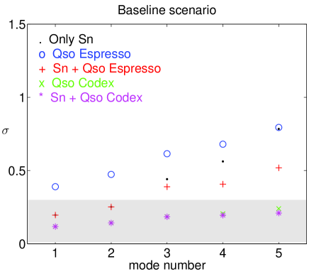
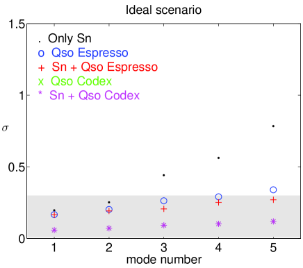
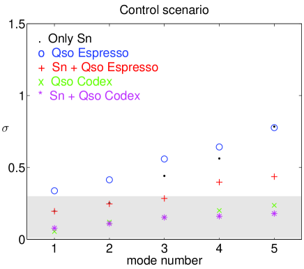
By inspecting Figs. 1 to 3 it can easily be understood that the baseline and control scenarios yield identical results for the magnitude of the modes’ errors. The ideal scenario, as expected, permits that more eigenmodes enter the region for which it is considered that modes are informative. In order to avoid an overburden of similar figures, we summarize the eigenvalue spectra for this parametrization (11) and parametrizations (12) and (13) in Tables 1 – 3. It can be noticed that the baseline and control scenarios for ESPRESSO cannot bring further information when compared with supernovae alone. Only in the ideal scenario and in combination with supernovae, can the number of useful modes raise above 2. The only exception is for parametrization (11) where the ideal ESPRESSO has 4 good modes. CODEX, however, will offer a set of high precision data which can on its own provide a large number of informative eigenmodes in either of the three scenarios. We can see that the results are fairly independent of the fiducial parametrization chosen though parametrization (11) allows, in general, a higher number of modes considered informative for a given combination of data.
| Beseline | Ideal | Control | |
|---|---|---|---|
| Sne | 2 | 2 | 2 |
| ESPRESSO | 0 | 4 | 0 |
| Sne + ESPRESSO | 2 | 5 | 3 |
| CODEX | 7 | 16 | 7 |
| Sne + CODEX | 9 | 18 | 10 |
| Beseline | Ideal | Control | |
|---|---|---|---|
| Sne | 2 | 2 | 2 |
| ESPRESSO | 0 | 1 | 0 |
| Sne + ESPRESSO | 2 | 3 | 2 |
| CODEX | 2 | 8 | 3 |
| Sne + CODEX | 4 | 10 | 5 |
| Beseline | Ideal | Control | |
|---|---|---|---|
| Sne | 2 | 2 | 2 |
| ESPRESSO | 0 | 2 | 0 |
| Sne + ESPRESSO | 2 | 4 | 2 |
| CODEX | 4 | 12 | 6 |
| Sne + CODEX | 6 | 14 | 7 |
Let us now look at the evolution of the eigenmodes for parametrization (11) and compare with the modes using supernovae data alone.
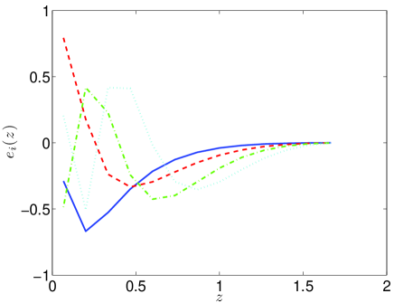
Because only the first two modes are considered informative, a reconstruction of the equation of state parameter using only supernovae can only be made reliably up to redshift 0.5 using the principal component approach. This value corresponds roughly to the position of the second mode’s peak in Fig. 4. We are interested in evaluating whether this limit can be relaxed with the help of QSO data using the ESPRESSO and CODEX spectrographs.
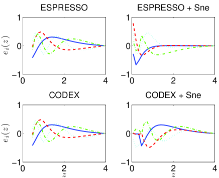
For the baseline scenario we see that only CODEX will permit a large number of modes considered useful. Inspecting Fig. 5 we see that a reconstruction of the equation of state parameter could be in principle possible up to redshift 2 corresponding roughly to the third peak of the third mode. The conclusions are similar for the ideal and control scenarios, see Figs. 6 and 7. In particular, only for the ideal scenario would ESPRESSO add information on the nature of dark energy.
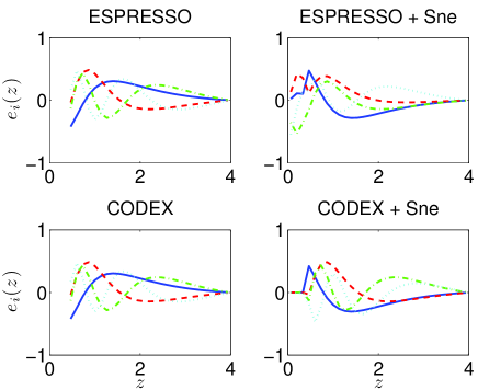
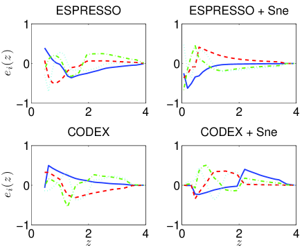
The form of the fiducial function is not determinant in the results and we would have reached the same conclusions had we illustrated the eigenmode evolution of parametrizations (12) or (13). We must emphasize, however, that the choice of threshold does play a role. Had we chosen a slightly higher value, say then the baseline scenario of ESPRESSO could indeed bring new information on the nature of dark energy when comparing to supernovae observations.
IV Reconstructing the equation of state parameter
Folowing Refs. Huterer and Starkman (2003); Albrecht and Bernstein (2007) one can now attempt a reconstruction by keeping only the most accurately determined modes (the ones with largest eigenvalues). To do this, we need to decide how many components to keep. We must point out that the weak point of this procedure consists in neglecting the high frequency modes. In a more recent analysis Crittenden et al. (2009) and perhaps more robust approach, all modes are kept and a correlation function describing fluctuations from a fiducial model is chosen. This method allows a more accurate reconstruction of the dark energy parameter over the whole range of redshifts covered by observations. We decided, however, to follow Refs. Huterer and Starkman (2003); Albrecht and Bernstein (2007) given the simplicity of the methods described there. This will be sufficient to support our main conclusion i.e., that a combination of supernovae and quasar data will improve on testing the time dependence of dark energy.
IV.1 Selection of components: risk vs. normalization
One may argue that the optimal value of modes to be kept corresponds to the value that minimizes the risk, defined as Huterer and Starkman (2003)
| (14) |
with
| (15) |
where the notation means that the sum in (2) runs from 1 to , and
| (16) |
The bias measures how much the reconstructed equation of state, , differs from the true one by neglecting the high and noisy modes and therefore, typically decreases as we increase . The variance of , however, will increase as we increase , since we will be including modes that are less accurately determined.
An alternative way to decide on the number of optimal modes is to choose the largest value for which the error is below unity, or equivalently, the RMS fluctuations of the equation of state parameter in such mode are
| (17) |
Having thus determined the optimal number of modes, we proceed with the normalization of the error following Ref. Albrecht et al. (2009) such that for the worse determined mode and normalize the error on the remaining modes by taking
| (18) |
The PCA allows us to optimize an experiment towards the range in redshift we are interested in. In our work, we will use a combination of supernovae and quasar absorption lines to understand how well the equation of state parameter will be constrained with forthcoming data on cosmological variation of fundamental parameters obtained with the spectrographs ESPRESSO for the VLT and CODEX for the E-ELT.
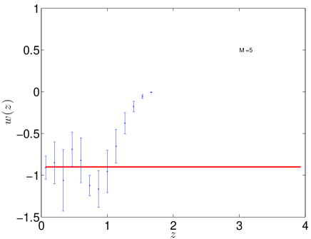
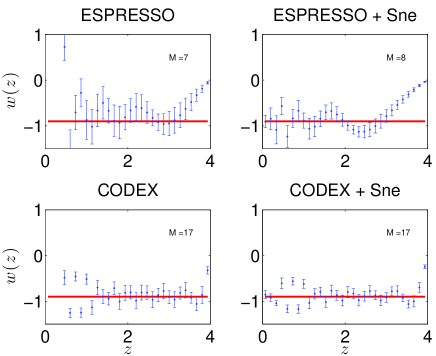
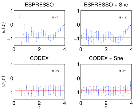
In Fig. 8 we illustrate the reconstruction using only supernovae for our fiducial model (11) and in Figs. 9 and 10 we show the result of the reconstruction for the two spectrographs and the two methods for the selection of the number of components. We can observe that, for this fixed number of bins, the reconstruction obtained using supernovae is only accurate up to redshift . In particular, because we neglect the poorly determined modes which are the ones with high amplitudes for bins of large redshift, the reconstructed equation of state parameter tends to zero for large redshift. This unavoidable feature of the PCA truncation method can be confused with a real increase in the equation of state at high redshift. As it was pointed out in Huterer and Starkman (2003), had we reconstructed instead, then would approach for large redshifts. Ideally we would like to extend the survey to large redshifts but unfortunately we only expect data from supernovas up to redshift .
Measurements from the quasar absorption lines, which are available for a larger redshift interval, provide in general a more reliable reconstruction. For our fiducial parametrizations of , these datasets can give a qualitatively accurate account of the evolution of the equation of state parameter to fairly high redshifts.
Comparing the various fiducial models for the same observational dataset shows that (as one would expect) the redshift up to which the reconstruction remains accurate depends in part on the correct underlying model, specifically on whether its equation of state remains close to a cosmological constant or approaches a dust-like behavior. However, comparing the CODEX and ESPRESSO cases show that one can go deeper in redshift by increasing the sensitivity of the measurements, since that allows one to add components to the reconstruction. In particular, the truncation problem mentioned earlier becomes less problematic as the reconstructed equation of state parameter no longer approaches zero for large redshifts. This is a true statement also for the alternative parametrizations.
The combination of supernovae with quasar absorption lines data further improves the determination of the equation of state parameter. In particular, we can now obtain information on all the way from up to . The reconstruction using CODEX, benefiting from an almost one order of magnitude improvement in the sensitivity of the QSO data points, is substantially better than the one obtained with ESPRESSO.
We can also compare the two methods of determining the optimal value of modes to keep in the reconstruction. We have seen before that the minimization of the risk method is a compromise between having an accurate equation of state reconstruction and having a small error bar in this reconstruction. The normalization of the error on the modes method, however, makes use of our prior prejudice that variations of larger than unity are unlikely. We observe, from comparing Fig. 9 to Fig. 10, to which correspond different methods, that the latter method picks more modes, which leads to a more accurate reconstruction. Since we are including additional modes with progressively larger errors, the reconstructed equation of state in this case also has larger error bars. In other words, the normalization method provides a more conservative and accurate approach, while the risk method provides (appropriately) a more aggressive approach.
From a practical point of view, the advantage of PCA techniques is that they may provide us with a simple computational tool to continually optimize an observational plan. In other words, given an ongoing observational campaign in which one has already observed a certain number of sources (with given uncertainties) one can use these tools to simulate improved datasets with the goal of determining how to best spend the remaining telescope time (reducing the uncertainty in measurements of particular sources) so as to achieve the best possible constraints on these models, given any relevant observational limitations.
V Conclusions
In the first part of our study we considered the threshold value presented in Ref. Crittenden et al. (2009) as a mean to determine how many modes can be considered good and informative in describing dark energy. This value, , is somehow arbitrary but serves our purpose to indicate that future precise measurements of the fine-structure constant, specially with CODEX, can add information on the nature of dark energy up to high redshifts when comparing to supernovae measurements.
In the second part of this work we have compared reconstructions of the equation of state parameter of dark energy using a principal component analysis. To this effect we used a combination of expected supernovae data and quasar absorption measurements of the fine-structure constant , expected to be available with the spectrographs ESPRESSO and CODEX. We considered several possible datasets and also two methods of choosing the best determined modes of the principal decomposition and studied the effect of the size of the error bars on the reconstruction.
Our analysis indicates that the normalization of the error on the modes method appears to give more accurate (closer to the fiducial value) but less precise (more conservative errors) reconstructions with respect to the risk minimization procedure. We also conclude that a reconstruction using quasar absorption lines is expected to be more accurate than using supernovae data. However, since the two types of measurements probe different (but overlapping) redshift ranges, combining them leads to a more complete picture of the evolution of the equation of state parameter between redshift zero and four.
A natural extension of this work is to include in addition cosmological measurements of , the ratio of the proton and electron masses Thompson et al. (2009). Measurements of will be fewer than those of but will all be at high redshift and fairly precise and are, therefore, expected to reduce the errors on the reconstruction of .
Although in this work we have focused on combining two datasets, we should also point out that they can also be used separately to provide independent reconstructions. Comparing the two reconstructions will then provide a consistency test, specifically for the assumption on the coupling between the scalar field and electromagnetism (given by Eq. 4). If so one can also obtain a measurement for the coupling parameter . A more detailed treatment of this case, as well as the application of the method to existing datasets, is left for forthcoming work.
Since a PCA reconstruction involves a truncation, it will not be precise at high redshifts. How much of a problem this is depends on the behaviour of the true equation of state: the reconstructed equation will always approach at high redshifts, while the true one may or may not do so in the redshift range being probed by the detaset under consideration. A relevant question for PCA studies is therefore how deep in redshift can one confidently go. In most previous works one has a fiducial model for that approaches by around , in which case supernovas perform well; however this is an optimistic assumption that need not be true. One of our key points is that, not knowing a priori what the correct equation of state will look like, there is strong interest in trying to reconstruct as deep as possible in redshift, and varying couplings are a possible way of doing that.
One must bear in mind that one should not compare the parametric-free PCA constraints with those obtained using parametrized equations of state. Perhaps a more direct comparison is with redshift binned . A good benchmark can be found in Fig. 17 of the work by Kowalsky et al. Kowalski et al. (2008), where one sees how poorly the high redshift behaviour of the equation of state is measured by current data.
Finally, our main conclusion is that, when one compares like with like, the inclusion of varying constants data allows a reliable reconstruction to be carried out to significantly higher redshifts. Admittedly, for these methods to be competitive will require very good quality measurements, which do not presently exist (although they are expected to be available in a few years), but this point applies both for the supernovas and for the varying couplings. In any case, the method is interesting on its own right, and should be further studied as the science cases of future facilities is developed.
Acknowledgements.
This work was done in the context of the FCT-DAAD cooperation grant ’The Dark Side of the Universe’ (reference 441.00 Alemanha), with additional support from project PTDC/FIS/111725/2009 from FCT, Portugal. The work of CM is funded by a Ciência2007 Research Contract, funded by FCT/MCTES (Portugal) and POPH/FSE (EC), and is also partially supported by grant PTDC/CTE-AST/098604/2008. LA and NJN are supported by Deutsche Forschungsgemeinschaft (project TRR33), and NJN is also partially supported by grants CERN/FP/116398/2010 and PTDC/FIS/102742/2008. The work of PP was partially funded by grant CAUP-09/2009-BII. CM acknowledges useful discussions with Paolo Molaro and Patrick Petitjean, particularly for defining the observational scenarios considered.References
- Carroll (2001) S. M. Carroll, Living Rev.Rel. 4, 1 (2001), eprint astro-ph/0004075.
- Copeland et al. (2006) E. J. Copeland, M. Sami, and S. Tsujikawa, Int.J.Mod.Phys. D15, 1753 (2006), eprint hep-th/0603057.
- Amendola and Tsujikawa (2010) L. Amendola and S. Tsujikawa, Dark Energy: Theory and Observations (Cambridge University Press, 2010).
- Clifton et al. (2011) T. Clifton, P. G. Ferreira, A. Padilla, and C. Skordis (2011), eprint 1106.2476.
- Martins (2002) C. J. Martins, Phil.Trans.Roy.Soc.Lond. A360, 2681 (2002), eprint astro-ph/0205504.
- Garcia-Berro et al. (2007) E. Garcia-Berro, J. Isern, and Y. Kubyshin, Astron.Astrophys.Rev. 14, 113 (2007).
- Uzan (2011) J.-P. Uzan, Living Rev.Rel. 14, 2 (2011), eprint 1009.5514.
- Martins and Molaro (2011) C. Martins and P. Molaro, From varying couplings to fundamental physics (Springer, 2011).
- Nunes and Lidsey (2004) N. J. Nunes and J. E. Lidsey, Phys. Rev. D69, 123511 (2004), eprint astro-ph/0310882.
- Avelino et al. (2006) P. P. Avelino, C. J. A. P. Martins, N. J. Nunes, and K. A. Olive, Phys. Rev. D74, 083508 (2006), eprint astro-ph/0605690.
- Avelino (2008) P. P. Avelino, Phys. Rev. D78, 043516 (2008), eprint 0804.3394.
- Nunes et al. (2009) N. J. Nunes, T. Dent, C. J. A. P. Martins, and G. Robbers, Memorie della Societa Astronomica Italiana 80, 785 (2009), eprint 0910.4935.
- Parkinson et al. (2004) D. Parkinson, B. A. Bassett, and J. D. Barrow, Phys. Lett. B578, 235 (2004), eprint astro-ph/0307227.
- Murphy et al. (2003) M. T. Murphy, J. K. Webb, and V. V. Flambaum, Mon. Not. Roy. Astron. Soc. 345, 609 (2003), eprint astro-ph/0306483.
- Murphy et al. (2004) M. T. Murphy et al., Lect. Notes Phys. 648, 131 (2004), eprint astro-ph/0310318.
- Srianand et al. (2007) R. Srianand, H. Chand, P. Petitjean, and B. Aracil, Phys. Rev. Lett. 99, 239002 (2007).
- Webb et al. (2010) J. Webb, J. King, M. Murphy, V. Flambaum, R. Carswell, et al., Phys.Rev.Lett. (2010), eprint arXiv:1008.3907.
- Reinhold et al. (2006) E. Reinhold, R. Buning, U. Hollenstein, A. Ivanchik, P. Petitjean, et al., Phys.Rev.Lett. 96, 151101 (2006).
- King et al. (2008) J. A. King, J. K. Webb, M. T. Murphy, and R. F. Carswell, Phys. Rev. Lett. 101, 251304 (2008), eprint 0807.4366.
- Thompson et al. (2009) R. I. Thompson et al., Astrophys. J. 703, 1648 (2009), eprint 0907.4392.
- Huterer and Starkman (2003) D. Huterer and G. Starkman, Phys. Rev. Lett. 90, 031301 (2003), eprint astro-ph/0207517.
- Albrecht and Bernstein (2007) A. Albrecht and G. Bernstein, Phys. Rev. D 75, 103003 (2007), eprint arXiv:astro-ph/0608269.
- Dvali and Zaldarriaga (2002) G. R. Dvali and M. Zaldarriaga, Phys. Rev. Lett. 88, 091303 (2002), eprint hep-ph/0108217.
- Chiba and Kohri (2002) T. Chiba and K. Kohri, Prog. Theor. Phys. 107, 631 (2002), eprint hep-ph/0111086.
- Anchordoqui and Goldberg (2003) L. Anchordoqui and H. Goldberg, Phys. Rev. D68, 083513 (2003), eprint hep-ph/0306084.
- Copeland et al. (2004) E. J. Copeland, N. J. Nunes, and M. Pospelov, Phys. Rev. D69, 023501 (2004), eprint hep-ph/0307299.
- Marra and Rosati (2005) V. Marra and F. Rosati, JCAP 0505, 011 (2005), eprint astro-ph/0501515.
- Dent et al. (2009) T. Dent, S. Stern, and C. Wetterich, JCAP 0901, 038 (2009), eprint 0809.4628.
- Bento and Felipe (2009) M. C. Bento and R. G. Felipe, Phys. Lett. B674, 146 (2009), eprint 0812.4827.
- Gould et al. (2006) C. R. Gould, E. I. Sharapov, and S. K. Lamoreaux, Phys. Rev. C74, 024607 (2006), eprint nucl-ex/0701019.
- Petrov et al. (2006) Y. V. Petrov, A. I. Nazarov, M. S. Onegin, V. Y. Petrov, and E. G. Sakhnovsky, Phys. Rev. C74, 064610 (2006), eprint hep-ph/0506186.
- Cristiani et al. (2007) S. Cristiani, G. Avila, P. Bonifacio, F. Bouchy, B. Carswell, et al., Nuovo Cim. B122, 1159 (2007), eprint 0712.4152.
- Liske et al. (2008) J. Liske, L. Pasquini, P. Bonifacio, F. Bouchy, R. Carswell, et al. (2008), eprint 0802.1926.
- Crittenden et al. (2009) R. G. Crittenden, L. Pogosian, and G.-B. Zhao, JCAP 0912, 025 (2009), eprint astro-ph/0510293.
- Albrecht et al. (2009) A. Albrecht et al. (2009), eprint 0901.0721.
- Kowalski et al. (2008) M. Kowalski et al. (Supernova Cosmology Project), Astrophys.J. 686, 749 (2008), eprint 0804.4142.