Magnetization Dynamics, Gyromagnetic Relation, and Inertial Effects

Abstract

The gyromagnetic relation - i.e. the proportionality between the angular momentum $\vec{L}$ (defined by an inertial tensor) and the magnetization $\vec{M}$ - is evidence of the intimate connections between the magnetic properties and the inertial properties of ferromagnetic bodies. However, inertia is absent from the dynamics of a magnetic dipole (the Landau-Lifshitz equation, the Gilbert equation and the Bloch equation contain only the first derivative of the magnetization with respect to time). In order to investigate this paradoxical situation, the lagrangian approach (proposed originally by T. H. Gilbert) is revisited keeping an arbitrary nonzero inertial tensor. A dynamic equation generalized to the inertial regime is obtained. It is shown how both the usual gyromagnetic relation and the well-known Landau-Lifshitz-Gilbert equation are recovered at the kinetic limit, i.e. for time scales above the relaxation time $\tau$ of the angular momentum.

The analogy between the dynamics of the magnetization in a magnetic filed on one hand, and the dynamics of a symmetrical spinning top in a gravitational field on the other hand, is often exploited in introductory courses on magnetism. The precession effect (i.e. the rotation of the extremity of a vector of constant modulus) is indeed easy to observe on a spinning top, while it is difficult to see with a ferromagnet because it would require observations at sub-nanosecond time scales. Stoehr However, the analogy seems to be incomplete because the dynamics of the symmetric spinning top implies inertial effects (e.g. nutation) while for a uniformly magnetized body, the dynamics of the magnetization is described by the time variation of the magnetization $d\vec{M}/dt$ (i.e. the velocity) and does not include the second derivative $d^{2}\vec{M}/dt^{2}$ (i.e. the acceleration). Doering In other terms, there is no inertia in the dynamic equation. The aim of this paper is to push the analogy to its logical end with the introduction of inertia inertial in the dynamics of uniform magnetization within the Lagrangian formalism.

The precession of a uniform magnetic moment $\vec{M}=M_{s}\vec{e}_{3}$ ($M_{s}$ is the magnetization at saturation and $\vec{e}_{3}$ the radial unit vector) under an effective magnetic field $\vec{H}$ is often presented as a consequence of the gyromagnetic relation $\vec{M}=\gamma\vec{L}$ that links the magnetization to the angular momentum $\vec{L}$. The constant $\gamma$ is the gyromagnetic ratio. The gyromagnetic relation and the value of the constant $\gamma=q/(2m)$ can be justified in a basic atomic model of an electron of charge $q$ and mass $m$ orbiting around a nucleus. This well-known model (see section IV below) constitutes the hypothesis of the Ampère molecular currents, validated by Einstein and de Haas in their famous experiments of 1915 - 1916. Einstein ; Frenkel In the general case, with both spin and orbital contributions in condensed material, the gyromagnetic ratio writes $\gamma=g\,q/(2m)$ where the $g$ factor accounts for the fact that the electron in a ferromagnet is a complex quasi particle. Ohanian ; Stoehr

Using the gyromagnetic relation, the application of Newton’s second law $d\vec{L}/dt=\vec{M}\times\vec{H}$ leads directly to the precession equation $d\vec{M}/dt=\gamma\vec{M}\times\vec{H}$. However the application of the Newton’s law to a rigid rotating body (typically the spinning top in a gravitational field), leads to a more complex gyroscopic equation that contains inertial terms. As will be shown below, the gyromagnetic relation also imposes inertia for the dynamics of the magnetization. This paradoxical situation can be clarified by re-introducing the inertia in the equation of the magnetization and explicitly going to the kinetic limit.

It is first useful to come back to the short history of the dynamic equation of the magnetization, especially with the introduction of the dissipation, since the precession equation $d\vec{M}/dt=\gamma\vec{M}\times\vec{H}$ cannot account for the rapid relaxation toward the equilibrium state of the magnetization (typically after a couple of precession cycles, i.e. after some nanoseconds, in usual ferromagnets). In 1935 Landau and Lifshitz proposed an equation for the dynamics of the magnetization that takes into account both the precession and the relaxation along the magnetic field: $d\vec{M}/dt=\tilde{\gamma}\vec{M}\times\vec{H}\,+\,h^{\prime}\vec{M}\times(\vec{M}\times\vec{H})$, where $h^{\prime}$ is a damping term (defined below) and $\tilde{\gamma}=\gamma$. Landau The basic argument used to derive the equation was to keep the modulus of the magnetization constant. The derivative $d\vec{M}/dt$ is hence perpendicular to the vector $\vec{M}$.

Two decades later, after the development of ferromagnetic resonance (FMR) experiments Bloembergen and motivated by the observation of systematic deviations from the above equation for high damping, T. L. Gilbert derived the equation that bears his name using a Lagrangian formalism. GilbertPhD ; Gilbert The dynamics of the magnetization is then described by the equation

$$\frac{d\vec{M}}{dt}=\gamma\vec{M}\times\left(\vec{H}-\eta\frac{d\vec{M}}{dt}\right)$$ (1)

with the introduction of the damping coefficient $\eta$.

The Landau - Lifshitz equation and the Gilbert equation are equivalent Miltat provided that $h^{\prime}=\frac{\alpha\gamma}{1+\alpha^{2}}$ and $\tilde{\gamma}=\frac{\gamma}{1+\alpha^{2}}$ where $\alpha=\gamma\eta M_{s}$ is the dimensionless Gilbert damping (note that $\tilde{\gamma}\neq\gamma$: this was the decisive improvement brought by Gilbert to the Landau-Lifshitz proposition).

In line with previous works performed by W. Döring, Doering Gilbert introduced the Lagrangian of a uniform ferromagnet with a kinetic energy $\mathcal{T}=\vec{L}\vec{L}:\bar{\bar{I}}^{-1}/2$, where $\bar{\bar{I}}$ is the inertial tensor. He then chose an ad-hoc tensor of inertia in such a way that the inertial terms disappear from the dynamic equation (i.e. such that the Landau-Lifshitz equation is recovered at the low damping limit). To do that, a sufficient condition is to set to zero the two first principal moments of inertia $I_{1}=I_{2}=0$ (but keeping a non-zero kinetic energy: $I_{3}\neq 0$). As pointed out by Gilbert himself Gilbert this puzzling condition does not seem to correspond to any realistic mechanical system (see footnote 7 : ”I was unable to conceive of a physical object with an inertial tensor of this kind”). In the subsequent report about Gilbert’s derivation, the ad-hoc and puzzling condition $I_{1}=I_{2}=0$ is explicitly stated despite its problematic character. In his presentation of the Gilbert equation published in 1960 in the American Journal of Physics, Brown Brown wrote ”We treat the rotating moment system as a symmetric top, with principal moments of inertia $A=B=0$, $C>0$. For a top made of classical mass particles, $A=B=0$ implies $C=0$; but this top is not made of classical mass particles.” In our notation $A\equiv I_{1}$, $B\equiv I_{2}$, $C\equiv I_{3}$. In the reference textbook of Morrish Morrish (edited from 1965 to 2002), we can read: ”A Lagrangian function, $\mathcal{L}$, consistent with the accepted equation of motion (equation (10-3.2)) can be obtained by considering the magnetic system as a classical top with principal moments of inertia $(0,0,C)$…”. In our notation $C\equiv I_{3}$, and the equation (10-3.2) is $d\vec{M}/dt=\gamma\vec{M}\times\vec{H}+damping$. Accordingly, the mechanical approach is not presented as a realistic physical model (as it should, according to the gyromagnetic relation), but seems to be introduced as a pedagogical analogy of an unspecified non-classical theory, that would give a physical interpretation to the puzzling Gilbert’s condition. Indeed, this strange condition is presented as a specific property of the magnetic moments that would be due to the fact that ” this top is not made of classical mass particles” .

This is probably the reason why, after more than half a century of intensive use of the Gilbert’s equation, the full derivation following Gilbert’s approach - with the complete set of principal moments of inertia (i.e. without ad-hoc assumption) - has not been proposed (see e.g. Ricci ; Miltat for recent presentations of the Gilbert’s derivation). However, as will be shown below, this derivation can be performed at an elementary level, as a direct application of the Lagrangian formalism. Although straightforward, this derivation is very instructive because it shows that the puzzling condition $I_{1}=I_{2}=0$ is not necessary to obtain the Gilbert equation. Instead, the Gilbert’s condition is replaced by the necessary physical condition under which a diffusion process can be described by a non-inertial diffusion equation. This condition is the usual kinetic limit that results in the requirement that the typical measurement times should be longer than the relaxation time $\tau$ of the momentum (here for the angular momentum $\tau=I_{1}/(\eta M_{s}^{2})$). Rubi In this picture, the precession with damping is simply a diffusion process in a field of force, for which the angular momentum has reached its equilibrium. This change of paradigm has two consequences. A first important consequence is that an inertial regime of uniform magnetic dipoles is expected, and should be observed at short enough time scales. Second, the classical mechanical approach is much more than a pedagogical analogy, and it could be used (beyond the gyromagnetic relation) for a deeper understanding of non-equilibrium magnetomechanics and related processes.

I The mechanical analogy

The mechanical model is sketched in Figure 1. A rigid stick of length $M_{s}$ with one extremity fixed at the origin is described by the angles $\theta$ and $\varphi$. The stick is precessing around the vertical axis at the angular velocity $\dot{\varphi}$ and is spinning around its symmetry axis at the angular velocity $\dot{\psi}$. The phase space of this rigid rotator is defined by the angles $\{\theta,\varphi,\psi\}$ plus the angular momentum $\vec{L}$. The relation between the angular momentum and the angular velocity $\vec{\Omega}$ is $\vec{L}=\bar{\bar{I}}\vec{\Omega}$ where $\bar{\bar{I}}$ is the inertial tensor.

I.1 The rotating frame

In the rotating frame, or body-fixed frame $\{\vec{e}_{1},\vec{e}_{2},\vec{e}_{3}\}$, the inertial tensor is reduced to the principal moments of inertia $\{I_{1},I_{2},I_{3}\}$. The symmetry of revolution imposes furthermore that $I_{1}=I_{2}$:

$$\bar{I}=\left(\begin{array}[]{ccc}I_{1}&0&0\\ 0&I_{1}&0\\ 0&0&I_{3}\end{array}\right)$$ (2)

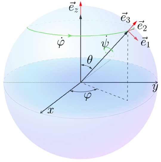
Figure 1: Illustration of the magnetomechanical analogy of a spinning stick that precesses around the $z$ axis. The coordinates of the stick in the space-fixed frame are parametrized by the angles $(\theta,\varphi,\psi)$ and the radius of the sphere is given by $M_{s}$. The body-fixed frame - denoted $\{\vec{e}_{1},\vec{e}_{2},\vec{e}_{3}\}$ - is spinning with the angular velocity $\dot{\psi}$ and is precessing around $\vec{e}_{z}$ with the angular velocity $\dot{\varphi}$.

In the fixed body frame, the angular velocity reads (see Fig. 1):

$$\begin{array}[]{ccc}\Omega_{1}&=&\dot{\varphi}\,sin\theta\,sin\psi+\dot{\theta}\,cos\psi\\ \Omega_{2}&=&\dot{\varphi}\,sin\theta\,cos\psi-\dot{\theta}\,sin\psi\\ \Omega_{3}&=&\dot{\varphi}\,cos\theta\ +\dot{\psi}\end{array}$$ (3)

The kinetic equation is obtained from the angular velocity: for any vector $\vec{M}$ of constant modulus carried with the rotating body, we have

$$\frac{d\vec{M}}{dt}=\vec{\Omega}\times\vec{M}$$ (4)

This equation can be inverted by cross multiplication by $\vec{M}$ and developing the double cross product. Since $\vec{M}=M_{s}\vec{e}_{3}$ we have:

$$\vec{\Omega}=\frac{\vec{M}}{M_{s}^{2}}\times\frac{d\vec{M}}{dt}+\Omega_{3}\vec{e}_{3}$$ (5)

I.2 The Lagrange equation

Following Gilbert and Döring, we introduce the Lagrangian of the system:

$$\mathcal{L}=\frac{1}{2}\left(I_{1}\left(\Omega_{1}^{2}+\Omega_{2}^{2}\right)+I_{3}\Omega_{3}^{2}\right)-V(\theta,\varphi)$$

where $V(\theta,\varphi)$ is the ferromagnetic potential energy that defines the effective magnetic field $\vec{H}=-\vec{\nabla}V$. The effective field $\vec{H}$ comprises the applied field, the anisotropy field, the dipolar field (or the demagnetizing field), the magneto-elastic contributions, etc.

The Lagrange equations are defined by :

$$\frac{d}{dt}\frac{\partial\mathcal{L}}{\partial\dot{q}_{i}}-\frac{\partial\mathcal{L}}{\partial q_{i}}+\frac{\partial\mathcal{F}}{\partial\dot{q}_{i}}=0$$ (6)

The $q_{i}$ refers to the three coordinates $\{\theta,\varphi,\psi\}$, and the components of the kinetic momentum are defined by the three derivatives $\frac{\partial\mathcal{L}}{\partial\dot{q}_{i}}=L_{i}$. The function $\mathcal{F}$ is the Rayleigh dissipative function. In a viscous environment, the Rayleigh function is defined by the damping coefficent $\eta$ such that $\mathcal{F}=\frac{\eta}{2}(\frac{dM}{dt})^{2}=\frac{1}{2}\eta M_{s}^{2}\left(\Omega_{1}^{2}+\Omega_{2}^{2}\right)$.

For the magnetomechanical model, the Lagrange equations read:

$$\begin{array}[]{ccc}\frac{d}{dt}[I_{1}\dot{\theta}]-I_{1}\dot{\varphi}^{2}\,sin\theta\,cos\theta+I_{3}\dot{\varphi}\,sin\theta\left(\dot{\varphi}\,cos\theta+\dot{\psi}\right)&=&-\frac{\partial\mathcal{F}}{\partial\dot{\theta}}-\frac{\partial V}{\partial\theta}\\ \frac{d}{dt}\left[I_{1}\dot{\varphi}sin^{2}\theta+I_{3}\left(\dot{\varphi}\,cos\theta+\dot{\psi}\right)cos\theta\right]&=&-\frac{\partial\mathcal{F}}{\partial\dot{\varphi}}-\frac{\partial V}{\partial\varphi}\\ \frac{d}{dt}\left[I_{3}\left(\dot{\varphi}\,cos\theta+\dot{\psi}\right)\right]&=&\,-\frac{\partial\mathcal{F}}{\partial\dot{\psi}}\,=0\end{array}$$ (7)

The right hand side of Eqs. (7) the last equation is equal to zero because there is no damping for spinning in the case of usual viscous environment. Condiff The quantity $L_{3}=I_{3}\Omega_{3}$ is then a constant of motion, and it can be written $L_{3}=M_{s}/\gamma$ without loss of generality.

II Kinetic equation and Gilbert’s assumptions

It is not trivial to see how to recover the Landau-Lifshitz equation from Eqs. (7), even at the low damping limit $\eta\rightarrow 0$. But it is clear that the inertial terms in the left hand side of Eqs.  (7) are not welcome from that point of view and should be removed. The best way to consider the inertial terms is to take the kinetic Equation Eq.  (5) with $\vec{L}=\bar{\bar{I}}\vec{\Omega}$:

$$\vec{L}=\frac{I_{1}}{M_{s}^{2}}\left(\vec{M}\times\frac{d\vec{M}}{dt}\right)+L_{3}\vec{e}_{3}$$ (8)

It is then rather immediate to see that the gyromagnetic relation $\vec{L}=\vec{M}/\gamma$ cannot be recovered without removing the first term on the right hand side. This was the great idea of Gilbert to assume that $I_{1}=0$. This is indeed a sufficient condition to kill the inertial terms, and the gyromagnetic relation is necessarily recovered with the definition $\gamma=M_{s}/L_{3}$ of the gyromagnetic ratio.

With both assumptions, the Lagrange equations Eqs. (7) rewrite:

$$\begin{array}[]{ccc}0&=&-\frac{M_{s}}{\gamma}\dot{\varphi}\,sin\theta-\frac{\partial\mathcal{F}}{\partial\dot{\theta}}-\frac{\partial V}{\partial\theta}\\ \frac{d}{dt}\left[\frac{M_{s}}{\gamma}cos\theta\right]&=&-\frac{\partial\mathcal{F}}{\partial\dot{\varphi}}-\frac{\partial V}{\partial\varphi}\\ \frac{d}{dt}\left[\frac{M_{s}}{\gamma}\right]&=&0\end{array}$$ (9)

Since in the rotating frame the effective field $\vec{H}=-\vec{\nabla}V$ reads $\{H_{1}=-\frac{1}{\sin(\theta)}\frac{\partial V}{\partial\varphi},H_{2}=\frac{\partial V}{\partial\theta},\}$, inserting Eq. (4) into Eq. (9) leads to :

$$\frac{d\vec{M}}{dt}=\gamma\vec{M}\times\left(\vec{H}-\eta\frac{d\vec{M}}{dt}\right)$$ (10)

This is the well-known Gilbert’s equation Eq. (1) obtained following the standard Lagrangian approach. GilbertPhD ; Gilbert ; Brown ; Morrish ; Ricci ; Miltat

However, the absence of inertia shows that the equation should be derived in the configuration space instead of the phase space (this is performed e.g. in references JEW ). Indeed, the dynamics is described by the two variables $\theta$ and $\varphi$ and not in the phase space defined by the five variables $\theta$, $\varphi$ and the components of $\vec{L}$. Accordingly, the gyromagnetic relation is - in this approach- not necessary (nor sufficient) for the derivation of the Gilbert equation.

III Beyond Gilbert’s assumption

In order to take into account the gyromagnetic relation, it is necessary to go beyond the Gilbert’s ad-hoc assumption and to set $I_{1}=I_{2}\neq 0$. The generalization of the Ampère molecular model from a quasi-one dimensional atomic model (the electric charge $q$ of mass $m$ distributed along the circular orbit) to a more realistic three dimensional atomic model - for which the orbits form an ellipsoid of revolution (the electric charge is now distributed in three dimensions) - imposes non-vanishing inertial moments $I_{1}=I_{2}\leq I_{3}$. Indeed, two parameters are necessary to take into account the amplitude of the magnetic moment ($M_{s}=\gamma/(\Omega_{3}I_{3})$) on one hand, and the anisotropy of the ferromagnetic material (with the dimensionless parameter $1-I_{1}/I_{3}$) on the other hand.

Note that for the magnetic system, the variables $\psi$ and $\dot{\psi}$ are not defined and should be removed from the model. Let us take for the sake of simplicity $\dot{\psi}=0$. Rquedotpsi With the relation $L_{3}=\frac{M_{s}}{\gamma}$, Eq. (7) gives:

$$\begin{array}[]{ccc}\dot{\Omega}_{1}&=&-\frac{\Omega_{1}}{\tau}+\Omega_{3}\left(1-\frac{I_{3}}{I_{1}}\right)\Omega_{2}-\frac{M_{s}}{I_{1}}H_{2}\\ \dot{\Omega}_{2}&=&-\frac{\Omega_{2}}{\tau}-\Omega_{3}\left(1-\frac{I_{3}}{I_{1}}\right)\Omega_{1}+\frac{M_{s}}{I_{1}}H_{1}\\ \Omega_{3}&=&\frac{M_{s}}{\gamma I_{3}}\end{array}$$ (11)

where the typical relaxation time $\tau\equiv\frac{I_{1}}{\eta M_{s}^{2}}$ has been introduced. The relaxation time $\tau$ is the typical time above which the diffusion approximation is valid, i.e. above which the angular momentum has relaxed toward the equilibrium state. inertial

Using $\dot{\vec{\Omega}}.\vec{e}_{3}=0$, Eq. (4), Eq. (5) and the time derivative of Eq. (5), Eq. (11) re-writes:

$$\frac{d\vec{M}}{dt}=\gamma\vec{M}\times\left[\vec{H}-\eta\left(\frac{d\vec{M}}{dt}+\tau\frac{d^{2}\vec{M}}{dt^{2}}\right)\right]$$ (12)

This is the Gilbert’s equation of the dynamics of the magnetization that includes the new inertial term $-\gamma\tau\,\vec{M}\times\left(d^{2}\vec{M}/dt^{2}\right)$.

IV Typical time scales

The limit of Eq. (12) for $t\gg\tau$, where $\tau=\frac{I_{1}}{\eta M_{s}^{2}}$ leads to the kinetic limit. Since the damping $\eta$ can be replaced by the usual dimensionless Gilbert coefficient $\alpha=\gamma\eta M_{s}$, we have $\tau=\frac{I_{1}}{I_{3}}\frac{1}{\alpha\Omega_{3}}$. A rigorous study of the asymptotic behavior (as a function of the parameters $\gamma\vec{H}$, $\tau^{-1}$ and $\eta$) is beyond the scope of this work. However it is sufficient to observe that the limit $\tau\rightarrow 0$ leads straightforwardly to the LLG equation:

$$\frac{d\vec{M}}{dt}\,\longrightarrow\,\gamma\vec{M}\times\left(\vec{H}-\eta\frac{d\vec{M}}{dt}\right)$$ (13)

In the same manner the vectorial gyromagnetic relation is recovered at the limit $\tau\rightarrow 0$. Eq. (8) gives:

$$\frac{d\vec{L}}{dt}=\eta\tau\,\left(\vec{M}\times\frac{d^{2}\vec{M}}{dt^{2}}\right)+\frac{1}{\gamma}\frac{d\vec{M}}{dt}\,\longrightarrow\,\frac{1}{\gamma}\frac{d\vec{M}}{dt}$$ (14)

The sufficient condition of validity of the Gilbert equation $I_{1}=0$ is hence replaced by the condition $\tau\rightarrow 0$ (i.e. $\tau\ll t$ for the relevant range of the parameters).

An estimation of the value of $\tau$ gives the typical time scale for which inertial effects can be observed. Here we come back to the simplest argument for the justification of the value of $\gamma$, namely the model of the Ampère molecular currents. This is a quasi-one dimensional atomic model, for which the atomic orbital moment is defined by the electronic charge $q$ orbiting around a nucleus at the distance $r$ with a velocity $v$. This system defines an electric loop that generates a magnetic moment $\vec{M}=\mathcal{I}S\,\vec{e}_{z}$, where $\mathcal{I}=qv/(2\pi r)$ is the electric current, $S=\pi r^{2}$ is the surface enclosed by the loop, and $\vec{e}_{z}$ is the vector normal to the loop. This leads to the microscopic magnetic moment $M_{s}=qvr/2$. If we take the Bohr radius $a_{0}$ and the electron velocity $v$ with the Heisenberg relation $mva_{0}\geq\hbar/2$, the Bohr magneton is obtained for the minimum value of the atomic magnetic moment $\mu_{B}=\gamma\hbar/2$. On the other hand, the angular moment of this system is $L_{3}=rmv$ and the ratio $M_{3}/L_{3}\equiv\gamma=q/(2m)$. The angular frequency $\Omega_{3}$ is given by $L_{3}=I_{3}~{}\Omega_{3}~{}=~{}\mu_{B}/\gamma$, i.e. $\Omega_{3}~{}=~{}\mu_{B}/(\gamma I_{3})$ where $I_{3}=ma_{0}^{2}$. We have $\Omega_{3}\approx 3\,10^{16}$ $rad/s$ and an order of magnitude of the typical times $\tau=\frac{I_{1}}{I_{3}}\frac{1}{\alpha\Omega_{3}}$ at which inertial effects should be observed is around a femtosecond (for a damping coefficient $\alpha$ such that $I_{1}/(I_{3}\,\alpha)\approx 0.1$).

V Conclusion

The paradoxical role played by the angular momentum for the dynamics of the magnetization has been studied in the light of the model introduced by T. H. Gilbert for the demonstration of the equation that bears his name. The demonstration has been reconsidered without the puzzling Gilbert’s assumption of vanishing first moments of inertia $I_{1}=I_{2}=0$ and $I_{3}\neq 0$. Instead, a general inertial tensor with the three arbitrary principal moments of inertia $\{I_{1},I_{1},I_{3}\}$ has been used. A generalized expression of the equation of the dynamics of the magnetization is obtained, that includes an inertial term: the mechanical analogy of the magnetic moment with the rigid rotator is complete. Both the usual expression of the Landau-Lifshitz-Gilbert equation and the usual gyromagnetic relation are recovered provided that a kinetic limit is performed for time scales much larger than the relaxation time of the angular momentum $\tau=I_{1}/(\eta M_{s}^{2})$. The typical time scale is found to be of the order of the femtosecond.

References

- (1) J. Stöhr, H. C. Siegmann, Magnetism. From Fundamental to Nanoscale Dynamics, Springer, Berlin 2006.
- (2) This is not the case for non-uniform magnetization (domain walls or antiferromagnets), for which a magnetic mass is defined. See the pioneering work of W. Döring: ”Über die trägheit der Wände zwischen Weisschen Bezirken” (On the inertia of walls between Weiss domains), Z. Natur. 3 373-379 (1948). Döring introduced the magnetic Lagrangian in this paper.
- (3) M.-C. Ciornei, J. M. Rubí, and J.-E. Wegrowe, Magnetization dynamics in the inertial regime: Nutation predicted at short time scales, Phys. Rev. B 83, 020410(R) 1- 4 (2011).
- (4) H. C. Ohanian, What is spin?, Am. J. Phys. 54, 500 - 505 (1986)
- (5) The gyromagnetic relation has been established through static magnetomechanical measurements, by S. J. Barnett (see Rev. Mod. Phys. 7, 129 (1935)), and A. Einstein and W. J. de Haas (Verh. d. D. Phys. Ges. 17, 152 (1915)).
- (6) V. Ya. Frenkel’ On the history of the Einstein-de Haas effect, Sov. Phys. Usp. 22, 580 - 587 (1979).
- (7) L. Landau and E. Lifshitz, On the theory of dispersion of magnetic permeability in ferromagnetic bodies, Phys. Z. Sowjet. 8, 153-169 (1935).
- (8) N. Bloembergen, On the ferromagnetic resonance in Nickel and supermalloy, Phys. Rev. 78, 572-580 (1950)
- (9) T. L. Gilbert, Formulation, foundations and applications of the phenomenological theory of ferromagnetism, PhD dissertation, Illinois Institute of Technology, June 1956, appendix B.
- (10) T. L. Gilbert, A phenomenological Theory of Damping in Ferromagnetic Materials, IEEE Trans. Mag. 40, 3443 (2004). The discussion related to the assumption is confined in the footnotes 7 and 8 of the 2004 paper. Note that the original reference in Physical Review is only an abstract: T. L. Gilbert, A Lagrangian formulation of the gyromagnetic equation of the magnetization fields” Phys. Rev. 100, 1243 (1955).
- (11) J. Miltat, G. Alburquerque, A. Thiaville, An introduction to microsmagnetics in the dynamics regime, in Spin dynamics in confined magnetic structures I, Eds. B. Hillebrands, K. Ounadjela, Springer, Berlin, 2002. The kinetic energy is introduced through the Lagrangian page 19 Eq. (37). The Lagrangian is such that (with our notations) and .
- (12) W. F. Brown Jr., Single-Domain Particles : New Uses of Old Theorems, Am. J. Phys. 28, 542-551 (1960), see page 549.
- (13) A. H. Morrish, ”The Physical Principles of Magnetism”, J. Wiley & Son, New York 1965 (original edition), reprinted in 1980 by R. E. Krieger Publishing Company, and IEEE Press New York 2001. End of the page 551.
- (14) T. F. Ricci and C. Scherer, A Stochastic Model for the Dynamics of Classical Spin , J. Stat. Phys. 67, 1201 (1992), page 1204-1208: ”In order to simulate the behavior of a classical spin, we take, for these equations, the limit , , and , but maintaining finite ”. In our notation .
- (15) J. M. Rubí, A. Pérez-Madrid, Inertial effects in non-equilibrium thermodynamics, Physica A 264 (1999) 492 - 502.
- (16) D. W. Condiff and J. S. Dahler, Brownian Motion of Polyatomic Molecules: The Coupling of Rotational and Translational Motions J. Chem. Phys. 44, 3988-4005 (1966).
- (17) J.-E. Wegrowe ”Spin transfer from the point of view of the ferromagnetic degrees of freedom”, Solid State Com. 150, 519- 523 (2010)
- (18) The full calculation with gives the same result. It is consistent with that found with a different approach in reference M.-C. Ciornei et al. Phys. Rev. B 83, 020410(R) (2011).