Towards a mesoscopic model of water-like fluids with hydrodynamic interactions

Abstract

We present a mesoscopic lattice model for non-ideal fluid flows with directional interactions, mimicking the effects of hydrogen-bonds in water. The model supports a rich and complex structural dynamics of the orientational order parameter, and exhibits the formation of disordered domains whose size and shape depend on the relative strength of directional order and thermal diffusivity. By letting the directional forces carry an inverse density dependence, the model is able to display a correlation between ordered domains and low density regions, reflecting the idea of water as a denser liquid in the disordered state than in the ordered one.

I Introduction

Water is a most common fluid, and yet one still full of mysteries. Indeed, water has been reckoned to exhibit dozens of anomalies, as compared to standard fluids, primarily the fact of being denser in the liquid than solid phase, exhibiting a density maximum at $4^{o}C$, i.e. above the freezing point (for a vivid non technical description, see Cart10). Although a fully comprehensive theory of water thermodynamics is still missing, there is an increasing consensus that most of these anomalies can be traced back to the peculiar nature of the hydrogen bond (HB). The HB interaction plays a vital role on structure formation within water. For instance, in water at low temperature, the HB’s lead to the formation of an open, approximately four-coordinated (tetrahedral) structure, in which entropy, internal energy and density decrease with decreasing temperature Poole94. The equilibrium thermodynamics, i.e. phase diagram, of water is exceedingly rich, and an ab-initio comprehensive analysis of its properties is beyond computational reach. As a result, many models have been developed Dill, including lattice ones, which display water-like behavior LGW; Sastry93; Franzese10. Such lattice models are typically based on a many-body lattice-gas Hamiltonian mimicking the essential features of water interactions, with no claim/aim of/at atomistic fidelity LGW2. To the best of our knowledge, these models have been employed mostly for the study of equilibrium properties, typically via Monte Carlo simulations. Yet, in most phenomena of practical interest, water flows and, most importantly, a variety of molecules, say colloids, ions and biopolymers, flow along with it, typically in nanoconfined geometries. In the biological context, it is well known that the competition between hydrophobic and hydrophilic interactions plays a crucial role in affecting the conformational dynamics of proteins Karplus; Ciepa; Rao. On a larger scale, hydrodynamic interactions are know to exert a significant effect on the collective dynamics and aggregation phenomena within protein suspensions. More generally, hydrodynamic interactions are crucial in the presence of confining walls, due to their strong coupling with resulting inhomogeneities PhysTod.

Based on the above, there is clearly wide scope for a minimal model of water behavior, capable of including hydrodynamic interactions and geometrical confinement, at a mesoscopic level (say tens of nanometers to tens of microns). In this respect, a remarkable mesoscopic methodology has emerged in the last two decades, in the form of minimal versions of the (lattice) Boltzmann kinetic equation ben92; che98; wg00; succi01. Such lattice Boltzmann equations (LBE’s) have proven fairly successful in simulating a broad variety of complex flows across scales, from macroscopic fluid turbulence, all the way down to biopolymer translocation in nanopores STATPHYS. The LB approach is mostly valued for its flexibility towards the treatment of complex geometries and seamless inclusion of complex physical interactions, e.g. flows with phase transitions. Such advantages are only accrued by the outstanding computational efficiency of the method, especially on parallel computers AMATI; COVEN. To the best of our knowledge, however, no LB model for water-like fluids has been developed as yet. In this paper, we present the first preliminary effort to fill this gap. More specifically, we develop a new LB framework including HB-like interactions, and explore the collective dynamics of the mesoscopic water-like fluids, both in free space (homogeneous) and nano-confined (heterogeneous) environments.

This paper is organized as follows. In Sec. II we present the basic elements of our mesoscopic approach, namely: in Sec. II.1 we state the transport equations as described by the Lattice Boltzmann model for non-ideal fluids, in Sec. II.2 we describe the directional interactions mimicking hydrogen-bonds and in Sec. II.3 we present the model for the dynamics of the orientational order parameter. The details of the numerical scheme are provided in Sec III. Our results are presented in Sec. IV where we first give a qualitative analysis of the mesoscopic model (Sec. IV.1) and an estimate of the numerical parameters to be used in the simulations (Sec. IV.2). We then present numerical results for homogeneous (Sec. IV.3) and inhomogeneous (wall-confined) scenarios (Sec. IV.4 and IV.5), without and with hydrodynamic flow. Finally, in Sec. V we provide an outlook of possible directions of future investigation.

II Mesoscopic model for water

II.1 Transport equations

Our fluid model is based on an extension of the lattice Boltzmann method for ideal fluids wg00; succi01. We use a two dimensional (2d) model on the D2Q9 lattice depicted in Fig. 1.

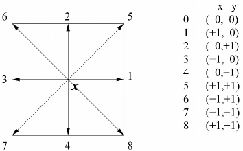
Figure 1: Distribution of the discrete molecular velocities ${\bf c}_{i}$, $i=0,..,8$, in the two-dimensional D2Q9 lattice.

At each grid node ${\bf x}$ the velocity distribution function $f_{i}({\bf x},t)$, i.e. the probability to find a particle at location ${\bf x}$, moving along the lattice direction defined by the discrete speed ${\bf c}_{i}$, is evolved according to the kinetic equation, with Bhatnagar-Gross-Krook (BGK) approximation bgk54; qia92:

$$f_{i}({\bf x}+{\bf c}_{i},t+\Delta t)-f_{i}({\bf x},t)=-\omega\,[f_{i}({\bf x},t)-f_{i}^{eq}({\bf x},t)]$$ (1)

where $\omega=\Delta t/\tau$, with the time step $\Delta t=1$, and $\tau$ the relaxation time towards local equilibrium. The relaxation time $\tau$ fixes the fluid kinematic viscosity $\nu=c_{s}^{2}(\tau-1/2)$, where $c_{s}$ is the sound speed of the lattice fluid. Here we have taken the mesh spacing $\Delta x=1$ so that $c_{s}=1/\sqrt{3}$.

The local equilibrium distribution function is a Maxwellian expanded to the second order in the fluid velocity wg00; succi01 and it is described by the distribution functions $f_{i}^{eq}$

$$f_{i}^{eq}=\begin{cases}w_{i}\rho\Big{[}1-\frac{3{\bf U}^{2}}{2\,c^{2}}\Big{]}\quad i=0\\ w_{i}\rho\Big{[}1+3\frac{{\bf c}_{i}\cdot{\bf U}}{c^{2}}+\frac{9({\bf c}_{i}\cdot{\bf U})^{2}}{2\,c^{4}}-\frac{3{\bf U}^{2}}{2\,c^{2}}\Big{]}\quad i=1,\ldots,8\end{cases}$$ (2)

The weights $w_{i}$ for the D2Q9 lattice are

$$w_{i}=\begin{cases}\frac{4}{9}~{}\quad i=0\\ \frac{1}{9}~{}\quad i=1,2,3,4\\ \frac{1}{36}\quad i=5,6,7,8\\ \end{cases}$$ (3)

and we take the propagation speed on the lattice $c=1$. The macroscopic variables in Eq. (2) are the fluid density $\rho$, and the fluid velocity ${\bf U}$, defined as follows:

$$\rho=\rho({\bf x},t)=\sum_{i=0}^{8}f_{i}({\bf x},t)$$ (4)

and:

$${\bf U}={\bf U}({\bf x},t)={\bf u}({\bf x},t)+{\tau\over\rho({\bf x},t)}{\bf F}({\bf x},t)$$ (5)

with

$$\rho({\bf x},t){\bf u}({\bf x},t)=\sum_{i=0}^{8}f_{i}({\bf x},t){\bf c}_{i}.$$ (6)

The forcing term ${\bf F}({\bf x},t)$ in Eq. (5) reflects the interparticle interactions. At a microscopic (molecular) level, these interactions are given by a combination of van der Waals and electrostatic forces, which take into account excluded volume, dispersion, directional hydrogen bonds and multipolar interactions. In this work, the cohesive forces prevailing in the aqueous environment are represented by a Shan-Chen pseudo-potential model sha93. The water-water cohesive forces are taken proportional to a free parameter ${\it G_{b}}$, and enter the momentum equations (5) via the forcing term

$${\bf F}({\bf x},t)=-G_{b}\psi({\bf x},t)\sum_{i=1}^{8}w_{i}\psi({\bf x}+{\bf c}_{i},t){\bf c}_{i}$$ (7)

where the normalization weights $w_{i}$ are taken as in Eq. (3) and $\psi$ is a function of the density, $\psi(\rho)=(1-\exp({-\rho})).$ Under these conditions, the fluid pressure receives a non-ideal contribution from potential energy interactions and takes the form:

$$p(\rho)=c_{s}^{2}\Big{(}\rho+{{\it G_{b}}\over 2}\psi^{2}(\rho)\Big{)}.$$ (8)

This non-ideal equation of state supports a liquid-vapor phase transition for $G_{b}<-4$ (negative $G_{b}$ values code for attraction) at a critical density $\rho_{c}=\ln 2$ in lattice units. Note that hard-core, short-range repulsive interactions in charge of stabilizing critical phase-separation are replaced by a self-driven saturation mechanism, whereby the force becomes vanishingly small as $\rho\gg 1$, as encoded in the exponential dependence of the pseudo-potential $\psi$ on the density $\rho$, and for a uniform density.

II.2 Directional interactions

The main distinctive feature of the present model consists in the inclusion of directional interactions, aimed at mimicking hydrogen bonds at a mesoscopic level. At the molecular level, the main effect of hydrogen-bonding (HB) between different water molecules is to align a donor (hydrogen atom) of a given water molecule to the acceptor (oxygen atom) of a neighboring molecule. The topology of these links is credited for exerting very profound effects on the collective behavior of water, and ultimately provides a basis for understanding its numerous anomalies. In particular, in three dimensions, at low temperature HB’s tend to favor tetrahedral structures (icy-water) which, being less packed than isotropic molecules, would explain why ice (the ordered phase) is less dense than liquid water (disordered phase). HB’s lead to the formation of complex and dynamic network structures, fueled by the unceasing breaking/formation of new HB’s. Since these are very short-lived events, we cannot expect them to be detectable at a mesoscopic level. At such a level, we expect to observe the dynamics of a suitable order parameter, which takes a zero value in the disordered phase and non-zero in the ordered one, the latter being promoted and sustained by mesoscopic directional interactions. Likewise, at a molecular level, temperature takes the form of random noise, promoting jumps between the different hydrogen-bond configurations (noise breaks the bond). At a mesoscopic level, though, noise takes the connotation of a diffusive process, driving the system towards a mesoscopically uniform state.

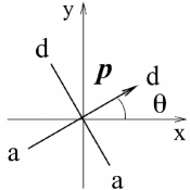
Figure 2: Model of a four-arm molecule. Two arms represents donors (d) and two arms are acceptors (a). The vector ${\bf p}=(p_{x},p_{y})$ is oriented in the direction of one donor, as shown in the figure.

To incorporate directional interactions (DI), we endow the lattice fluid with internal degrees of freedom, in charge of responding to orientational forces. These degrees of freedom are modeled in terms of four square-planar oriented bonding arms, as illustrated in Fig. 2. The bonding arms of each “molecule” are either ‘donor’-like or ‘acceptor’-like, to indicate hydrogen or oxygen type behavior, respectively. Since the four arms are rigid, they are uniquely identified by a single parameter, e.g. the angle $\theta$ formed by, say, the first arm with the $x$ coordinate axis. However, such an angle is not a convenient order parameter because of its periodicity. As a result, we have introduced a vector order parameter ${\bf p}=(p_{x},p_{y})$, pointing in the direction of one donor bonding arm (see Fig. 2). The angle $\theta$ relates to the vector ${\bf p}$ through $\theta=\tan^{-1}(p_{y}/p_{x})$. The interaction between two molecules located, respectively, at ${\bf x}$ and ${\bf x}_{i}$, with ${\bf r}_{i}={\bf x}_{i}-{\bf x}$, is described by the following interparticle pseudo-potential dak08:

$$V_{HB}({\bf x},{\bf x}_{i}) =\phi(\rho({\bf x}))\phi(\rho({\bf x}_{i}))\exp\Big{[}-{(r_{i}-R_{HB})^{2}\over 2\sigma^{2}_{R}}\Big{]}$$ (9)

$$\times\Big{(}\sum_{k=1}^{4}\sum_{k^{\prime}=1}^{4} \epsilon_{HB}(k,k^{\prime})\exp\Big{[}-\Big{(}{{\bf\hat{n}}_{k}\cdot{\bf r}_{i}\over r_{i}}-1\Big{)}^{2}{1\over 2\sigma^{2}_{\theta}}\Big{]}$$

$$\times\exp\Big{[}-\Big{(}{{\bf\hat{n}}_{i,k^{\prime}}\cdot{\bf r}_{i}\over r_{i}}+1\Big{)}^{2}{1\over 2\sigma^{2}_{\theta}}\Big{]}\Big{)}$$

where $r_{i}=|{\bf r}_{i}|$ and ${\bf\hat{n}}_{k}$ (${\bf\hat{n}}_{i,k^{\prime}}$), with $k\,(k^{\prime})=1,..,4$, are the unit vectors indicating the orientation of the four bonding arms of a molecule at grid node ${\bf x}$ (${\bf x}_{i}$) (see Fig. 3). $R_{HB}$ is the equilibrium radial distance of the HB’s, and $\sigma_{R}$ and $\sigma_{\theta}$ control the radial and angular decay of the interactions around such equilibrium (stiffness).

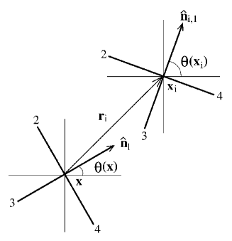
Figure 3: Sketch of two model “molecules” interacting via hydrogen-bond potential.

The matrix $\epsilon_{HB}(k,k^{\prime})$ is introduced to distinguish between donors (arms $1$ and $2$) and acceptors (arms $3$ and $4$). The interaction energy between donors and acceptors is equal to the constant $\varepsilon_{HB}<0$, whereas the interaction between two donors or two acceptors is set to zero.

To include the density-dependent propensity of water to form ordered states, which reflects the fact that tetrahedral ordered structures are less compact than isotropic disordered ones (the two liquid phases of water), we have introduced in Eq. (9) the weight function $\phi(\rho)$

$$\phi(\rho)={1\over 1+e^{-\alpha(\frac{\rho_{\rm max}-\rho}{\rho_{\rm max}-\rho_{\rm min}})}}$$ (10)

where $\rho_{\rm max}$ and $\rho_{\rm min}$ are the maximum and minimum density of the fluid under the chosen conditions and $\alpha>0$ is a parameter controlling the range of the density variation, which we have set equal to $10$ to implement a steeply decaying function.

We can now further justify our choice of the vector order parameter, ${\bf p}$, by noting that the potential in Eq. (9), with $R_{HB}=\sqrt{2}$, has four minima, corresponding to $\theta=\pi/4,3\pi/4,5\pi/4$ and $7\pi/4$. As a result, $\cos\theta$ alone cannot distinguish between these four, leaving two of them degenerate, unless $\sin\theta$ is also specified. Clearly, the two component vector ${\bf p}$ does not suffer of such limitation.

The magnitude of the total torque on ${\bf p}({\bf x},t)$ due to the HB interaction with its eight neighbors reads as follows:

$$\Delta\theta({\bf x},t)=C_{T}\;\sum_{i=1}^{8}c_{i}\Delta tF_{i}({\bf x},t)$$ (11)

where $C_{T}$ is a constant to be discussed shortly, $c_{i}=|{\bf c}_{i}|$, $\Delta t=1$ and $F_{i}({\bf x},t)$ is the angular component of the force between site ${\bf x}$ and ${\bf x}_{i}$, given by

$$F_{i}({\bf x},t)=-\sum_{k=1}^{4}{\partial V_{HB}({\bf x},{\bf x}_{i})\over c_{i}\partial\theta_{k}}$$ (12)

where $\theta_{k}=\tan^{-1}(n_{ky}/n_{kx})$, $k=1,..,4$. Thus

$$F_{i}({\bf x},t)=-\sum_{k=1}^{4}{\partial V_{HB}({\bf x},{\bf x}_{i})\over c_{i}\partial cos\alpha_{k}}{dcos\alpha_{k}\over d\theta_{k}}$$ (13)

with $\alpha_{k}$ the angle in between the unit vector in direction ${\bf\hat{n}}_{k}$ and the velocity ${\bf c}_{i}$

$$cos\alpha_{k}={{\bf\hat{n}}_{k}\cdot{\bf c}_{i}\over c_{i}}={n_{kx}c_{ix}+n_{ky}c_{iy}\over c_{i}};$$ (14)

here, $n_{kx}=cos\theta_{k},\,\,\,n_{ky}=sin\theta_{k}$. This gives

$$c_{i}F_{i}({\bf x},t)=\phi(\rho({\bf x}))\phi(\rho({\bf x}_{i}))\exp\Big{[}-{(c_{i}-R_{HB})^{2}\over 2\sigma^{2}_{R}}\Big{]}\times$$ (15)

$$\Big{(}\sum_{k=1}^{4}\sum_{k^{\prime}=1}^{4}\epsilon_{HB}(k,k^{\prime})2(\cos\alpha_{k}-1)\exp\Big{[}-\frac{(cos\alpha_{k}-1)^{2}}{2\sigma^{2}_{\theta}}\Big{]}$$

$$\times\Big{[}{-c_{ix}\sin\theta_{k}+c_{iy}\cos\theta_{k}\over c_{i}}}\Big{]}{\exp\Big{[}-\Big{(}{{\bf\hat{n}}_{i,k^{\prime}}\cdot{\bf c}_{i}\over c_{i}}+1\Big{)}^{2}{1\over 2\sigma^{2}_{\theta}}\Big{]}\Big{)}.$$

II.3 Dynamics of the order parameter

The idea underlying the present approach is that the mesoscopic description of directional interactions is reflected by the hydrodynamic equation of the vector ${\bf p}$. Such an equation must include three main effects: macroscopic advection, bond formation due to directional interactions and bond-breaking due to thermal noise. The resulting transport equation reads as follows

$${\partial{\bf p}\over\partial t}+{\bf u}\cdot\nabla{\bf p}={\bf T}+{\bf D}.$$ (16)

The two terms on the right hand side represent the deterministic torque, ${\bf T}$, due to the hydrogen-bond interaction, and thermal diffusion, ${\bf D}$, due to translational motion. As a result, the water-like fluid is characterized by the density $\rho$, the velocity ${\bf U}$ and the rotational vector ${\bf p}$. The equation (16) is evolved concurrently with the LB equation (1) for the fluid density and velocity.

II.3.1 Deterministic torque

The torque is represented by the force in Eq. (LABEL:rotation) which is inserted in the equations of motion for ${\bf p}$, after projection of its components along the $x$ and $y$ directions. The two components can be computed as illustrated in Fig. 4. The molecule rotates from the initial orientation $\theta=tan^{-1}(p_{y}/p_{x})$ to $\theta+\Delta\theta$. The angle $\Delta\theta$ is larger than $0$ for counterclockwise rotation, whereas $\Delta\theta<0$ for clockwise rotation. By making use of suitable trigonometric relationships, one obtains:

$$T_{x} =-2|{\bf p}|sin{\Delta\theta\over 2}sin\Big{(}{\Delta\theta\over 2}+\theta\Big{)}$$ (17)

$$T_{y} =\ 2|{\bf p}|sin{\Delta\theta\over 2}cos\Big{(}{\Delta\theta\over 2}+\theta\Big{)}.$$ (18)

As discussed previously, the torque is zero when the angle $\theta$ is in one of the four degenerate minima $\theta_{k}=(2k-1)\pi/4$, $k=1,4$.

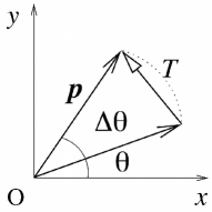
Figure 4: Deterministic rotation, ${\bf T}$, of the molecule whose initial orientation is $\theta=tan^{-1}(p_{y}/p_{x})$. Note that $|{\bf T}|=2|{\bf p}|\sin(|\Delta\theta|/2)$.

II.3.2 Thermal diffusivity

At a molecular scale, temperature acts as a HB-breaking noise which promotes transitions between different bond configurations. At a mesoscopic level, such bond-breaking effect manifests itself as a diffusion process, driving the system towards an isotropic, disordered state $\langle\cos\theta\rangle=\langle\sin\theta\rangle=0$, where brackets stand for ensemble averaging over a mesoscopic volume of fluid. As a result, in our model thermal diffusion is represented in standard laplacian form ${\bf D}=D_{p}\Delta{\bf p}$, where $D_{p}$ is the kinematic diffusivity of the vector ${\bf p}$, to be detailed shortly.

II.3.3 Hydrodynamic interactions

Hydrodynamic interactions are automatically included by moving the vector ${\bf p}$ along with the fluid velocity ${\bf U}$, resulting from the LB advection equation (1). These interactions are expected to play a major role in transport phenomena, with the fluid in motion and/or suspended bodies moving along with it. In the present study, however, we devote special attention to a simpler scenario, namely the competition between directional interactions and thermal diffusion. Such competition is also analyzed in the presence of hydrodynamic flows (Poiseuille), but mostly for illustrative purposes. Quantitative investigation of the highly complex phenomena resulting from the concurrent effects of directional interactions, diffusion and hydrodynamic transport, are left to future studies.

III Numerical scheme for the order parameter

The equation (16) for ${\bf p}$ is essentially an advection-diffusion-reaction equation, for which a wide variety of numerical methods is available, in particular, the so-called, moment propagation method, PAGO; PAGO2. For the sake of uniformity with the advection equation described in Sec. II.1, and also to secure very low numerical diffusivity, we have opted for a LB integrator also for the equation of the order parameter. Consequently, we integrate the equation of motion for ${\bf p}=(p_{x},p_{y})$ by a lattice Boltzmann scheme, applied separately to the two components of the vector. This means that, using the same D2Q9 lattice geometry of Sec. II.1, we define two sets of density distribution functions $g_{x,i}({\bf x},t)$ and $g_{y,i}({\bf x},t)$, $i=0,..,8$, respectively for $p_{x}$ and $p_{y}$, such that

$$p_{x}=p_{x}({\bf x},t)=\sum_{i=0}^{8}g_{x,i}({\bf x},t)$$ (19)

$$p_{x}({\bf x},t){\bf u}({\bf x},t)=\sum_{i=0}^{8}g_{x,i}({\bf x},t){\bf c}_{i}.$$ (20)

The kinetic equation for $g_{x,i}$ is:

$$g_{x,i}({\bf x}+{\bf c}_{i},t+1)-g_{x,i}({\bf x},t) =$$ (21)

$$-\omega_{p}(g_{x,i}({\bf x},t)- g_{x,i}^{eq}({\bf x},t))+T_{i}^{x}$$

where $T_{i}^{x}=w_{i}T_{x}$ is the $x$ component of the deterministic rotation, $\omega_{p}=1/\tau_{p}$, with $\tau_{p}$ the relaxation time towards local equilibrium, described by the density function

$$g_{x,i}^{eq}=p_{x}w_{i}\Big{[}1+{{\bf c}_{i}\cdot{\bf U}\over c_{s}^{2}}\Big{]},\quad\forall i.$$ (22)

Similar expressions hold for $p_{y}$ by replacing $x$ with $y$.

The hydrodynamic limit of this LB model for ${\bf p}$ yields the following continuum macroscopic equations:

$${{\partial{\bf p}}\over\partial t}+{\bf u}\cdot\nabla{\bf p}={\bf T}+D_{p}\Delta{\bf p},$$ (23)

with $D_{p}=c_{s}^{2}(\tau_{p}-1/2)$. An appealing aspect of LB is that one can tune the diffusivity to very small values by choosing

$$\tau_{p}={1\over 2}+\epsilon,$$ (24)

with $\epsilon$ typically of the order $1/N$, $N$ being the number of lattice sites per linear dimension.

We note that diffusivity is the emergent manifestation of microscopic noise, and acts in such a way as to smear out spatial gradients of the vector ${\bf p}$. One could still add a stochastic source to the rhs of equation (16), in order to model random noise. This, however, would not be consistent with the mesoscopic aim of the present model.

IV Numerical results

IV.1 Analysis of the model

Before discussing the details of the simulation results, a few general comments on the expected qualitative scenario are in order. The vector p moves with the fluid and diffuses at a rate fixed by the diffusivity $D_{p}$. At the same time, it rotates under the effect of the torque associated with directional interactions (DI) with the neighboring fluid sites. In the absence of DI’s, and with the fluid at rest ${\bf u}=0$, the order parameter would tend to a uniform state (disorder), as dictated by thermal diffusivity. DI’s, on the other hand, tend to place the system on local minima of the interaction potential, thereby giving rise to metastable ordered domains. The torque, which depends only on angular degrees of freedom, takes $\theta(x,y;t)$ to the local minimum closest to the initial condition $\theta(x,y;t=0)$. As a consequence, after an initial transient stage, the system settles down into its local minima, with no transitions between them. Indeed, transitions between different minima can be detected only in the initial stage, in which diffusion is still capable of affecting the evolution of $\theta$ towards different minima, because the system is still sufficiently far from equilibrium. Once this transient is over, the system freezes into a metastable crystal-like state. In this way, the system attains a state of coexistence between short-range uniformity and long-range disorder. Within each domain, the system remains uniform around the corresponding local minimum angle. On the other hand, the spatial distribution of the domains has a fairly disordered pattern, depending on the initial conditions and the (inverse) strength of the diffusion. A richer scenario, i.e. a longer transient with more inter-domain disorder, could be enforced by increasing the number of HB arms, so as to enhance the number of angular minima, hence their mutual competition. This would give rise to a more disordered system, but would not change once it falls into the closest minimum, the system stays forever.

IV.2 Numerical estimate of the simulation parameters

The quantitative details of the scenario previously described depend on the specific values of the parameters governing the physics of the system, primarily the relative strength of DI’s versus diffusion, namely $\varepsilon_{HB}/kT$. In the lattice Boltzmann model $kT=1/3$. In physical units, at ambient temperature $T=300K$, $kT\simeq 2,3KJ/mol$. For a water dimer, the potential energy of the hydrogen bond is of the order of $60KJ/mol$, whereas the free energy can be estimated as $\Delta F\sim kT/2$ rao10. In the present model, the role of the free energy, i.e. the energy difference between bounded and unbounded states, is played by the parameter $\varepsilon_{HB}$ in Eq. (9). Therefore, with $\varepsilon_{HB}=-0.1$, we fulfill the condition $\varepsilon_{HB}\sim\Delta F$.

The factor $C_{T}$, that, according to Eq. (11), weights the effect of the torque, is estimated via the momentum equation

$$I{d^{2}\theta\over dt^{2}}={\cal T}-I\gamma{d\theta\over dt}$$ (25)

where $I\simeq Ma^{2}$ is the moment of inertia, $\gamma$ the drag coefficient and ${\cal T}$ the torque. Thus, upon replacing infinitesimal with finite increments, at steady state, we obtain $\Delta\theta\simeq{{\cal T}\over I\gamma}\Delta t$. With $M=1$ and $a=1$, this yields $C_{T}\propto 1/\gamma$ (see Eq. (11)).

Next, we estimate the relative effect of the torque with respect to diffusion. First of all, by Taylor expansion, close to the minimum of ${\cal T}$, Eq. (25) gives ${d\theta\over dt}={{\cal T^{\prime}}\over I\gamma}\Delta\theta$ where ${\cal T^{\prime}}\equiv(d{\cal T}/d\theta)|_{\theta_{eq}}$. Therefore, the strength of the deterministic rotation can be quantified by the relaxation time $\tau_{T}$ ${1\over\tau_{T}}\equiv{{\cal T^{\prime}}\over I\gamma}$. On the other hand, the diffusion time scale in Eq. (16) can be computed according to ${1\over\tau_{D}}\sim{D_{p}\over w^{2}}$, with $w$ the width of the interface, typically of the order of $5$ lattice units in LB simulations. The ratio between diffusive and deterministic forcing is then given by

$${\tau_{T}\over\tau_{D}}={I\gamma D_{p}\over{\cal T^{\prime}}{w}^{2}}={I\gamma D_{p}\sigma_{\theta}^{2}\over|\varepsilon_{HB}|{w}^{2}}$$ (26)

where the second equality comes by dimensional analysis from Eq. (9), which leads to ${\cal T^{\prime}}\simeq|\varepsilon_{HB}|/\sigma_{\theta}^{2}$. In our numerical simulations, this ratio is changed by tuning two parameters, the strength of DI’s via $\varepsilon_{HB}$ and the diffusivity, via the parameter $\epsilon$. Finally, we set $\gamma=1$ for numerical convenience.

IV.3 Homogeneous scenario

We first consider the case of a bulk fluid without density-dependent interactions, i.e. where $G_{b}=0$ and $\phi(\rho)=1$. The heterogeneous case will be considered in Sec. IV.4. To study the effect of the different contributions to the dynamics of the order parameter, we start from the random initial condition shown in the top panels of Fig. 5, and consider the four different scenarios described below.

Run (a): DI’s only, no diffusion. Diffusion is set to zero and the dynamics of the vector ${\bf p}$ (hence of the $\theta$-domains) is dictated solely by the torque.

Run (b): small diffusivity. Diffusion is turned on ($\epsilon=0.01$), but the torque still dominates the dynamics ($\varepsilon_{HB}=-0.1$).

Run (c): large diffusivity. Diffusion ($\epsilon=0.01$) now dominates over torque ($\varepsilon_{HB}=-0.0001$).

Run (d): No DI’s, diffusion only. The system dynamics is entirely dictated by diffusion ($\epsilon=0.01$).

The parameters for these simulations are collected in Table 1.

Run	$\epsilon$	$V_{HB}$	$\varepsilon_{HB}$	$\tau_{T}/\tau_{D}$
(a)	$0$	ON	$-1\times 10^{-1}$	$0.0$
(b)	$0.01$	ON	$-1\times 10^{-1}$	$10^{-5}$
(c)	$0.01$	ON	$-1\times 10^{-4}$	$10^{-2}$
(d)	$0.01$	OFF	–	$\infty$

Table 1: Simulation parameters. The parameter $\epsilon$ fixes the numerical diffusivity (see Eq. (24)); $\tau_{T}/\tau_{D}$ is the relative strength of the deterministic torque to the diffusive term (see Eq. (26)). The drag coefficient is $\gamma=1$, with $C_{T}=1/\gamma$ in Eq. (11). When the HB potential $V_{HB}$ is switched on (see Eq. 9), we used the values $\sigma_{\theta}=\sigma_{R}=0.12$, $R_{HB}=\sqrt{2}$ and we set $\phi(\rho)=1$ to first consider the homogeneous scenario. The value of $\varepsilon_{HB}$ is given in the table. The lattice sizes were $N_{x}=N_{y}=64$ in all cases.

Figure 5: Configuration of $\theta$ in a $64^{2}$ homogeneous system, shown as contour plot (left), detail of the orientation of the four-armed “molecules” (middle, only donor arms are represented), and histogram (right). Starting from the same initial ($n$=0) random configuration shown in the top panels, we report the equilibrium configurations in the following two cases; Central panels: Run (a), the scenario with $\epsilon_{HB}=-1\times 10^{-1}$ and no diffusion in the dynamics of ${\bf p}$ (i.e. $\epsilon=0$). Equilibrium is reached after $n\approx 10^{3}$ steps. Bottom panels: Run (b), the scenario with $\epsilon_{HB}=-1\times 10^{-1}$ and diffusion with $\epsilon=0.01$. Equilibrium is reached after $n\approx 10^{4}$ steps. Note that in both cases the histograms are peaked around the four equilibrium values $\theta=\pi/4,3\pi/4,5\pi/4,7\pi/4$, but the size of the domains increases when diffusion is turned on. Also, the peaks of the histogram broaden with increasing diffusion, indicating thicker domain boundaries.

The equilibrium configurations for $\theta$ in Run (a) and Run (b) are shown in Fig. 5, together with the (random) initial configuration for all runs presented in this section. As expected, the directional interactions drive the system towards a disordered collection of uniform, ordered domains, i.e. within each domain $\theta$ takes the same value, but domains with different $\theta$ coexist within a disorderd global pattern, in which all four minima are roughly equally populated (as shown by the histograms). As discussed previously, the spatial distribution of the ordered domains reflects the initial condition, since $\theta$ is attracted to the minimum closest to its initial value, and once there, it stops evolving because the system is deterministic (no stochastic fluctuations). This corresponds to an arrested-coarsening scenario, as observed in many slow-relaxing materials, including water. In the absence of diffusion, coarsening is virtually quenched, and the resulting domains are very small and very close to the initial condition.

When diffusion is turned on, the system experiences additional freedom to evolve away from the initial condition. As a result of diffusive transport, coarsening can now take place, as indicated by the increased size of the uniform domains. Since DI’s are still dominant, the global pattern remains disordered. As expected, the size of the ordered domains depends on the relative strength of the HB to the thermal diffusion. Whenever diffusion dominates over the HB formation, coarsening can proceed up to the point where all domains merge into a single one, i.e. a uniform value of $\theta$ all over the region occupied by the fluid. This behavior is illustrated in Fig. 6. The final value of $\theta$ attained by the fluid corresponds to one of the four equilibrium angles of $V_{HB}$, and its specific value is selected by the initial condition. Also note that during its relaxation to global equilibrium, the system first reaches local equilibrium (shown by the peaks in the histogram around the metastable values of $\theta$), and then the ordered domains grow and merge, with the largest one absorbing the others. Although coarsening can proceed up to complete uniformity, the system still keeps track of HB interactions, in that the final $\theta$ cannot just take any value, but only one of the four degenerate minima. This means that, even upon averaging over initial conditions, the system remains non-ergodic, meaning by this that the probability distribution function (pdf) $P(\theta)$ is given by a combination of the four Dirac’s deltas, $P(\theta)=\frac{1}{4}\sum_{k=1}^{4}\delta(\theta-\theta_{k})$, with $\theta_{k}=(2k-1)\frac{\pi}{4}$, $k=1,4$. This scenario lies at other extreme as compared to the no-DI’s situation. As illustrated in Fig. 7, diffusion drives the system to a uniform state, with a relaxation dynamics similar to the case with weak directional interactions (cfr. with Fig. 6). However, in this case, the intermediate and final values of $\theta$ can take any value between $[0,2\pi]$, depending on the initial conditions. On a statistical basis, this is very different from the case of weak DI’s because ensemble averaging over initial conditions would now produce a uniform pdf, $P(\theta)=\frac{1}{2\pi}$.

We wish to emphasize that in the case of diffusion-dominated scenarios, the steady-state solution of Eq.(23) reads simply as $p_{x}\equiv p\cos\theta=const$ and $p_{y}\equiv p\sin\theta=const$, where $const$ means constant in time and space. This means that both the magnitude $p$ and the orientation $\theta$, are uniform in space. Such uniformity does not correspond to any microscopic “symmetry-breaking”, but simply reflects the diffusive structure of the mesoscopic equation of motion of the parameter ${\bf p}$. Indeed, in the diffusion-dominated scenario, isotropy is recovered by averaging upon initial conditions.

The results discussed in this section show that the present LB model with directional interactions is capable of sustaining long-lived, metastable states in the form of a disordered collection of uniform domains, whose asymptotic size and spatial distribution is controlled by the relative strength of directional interactions versus diffusion.

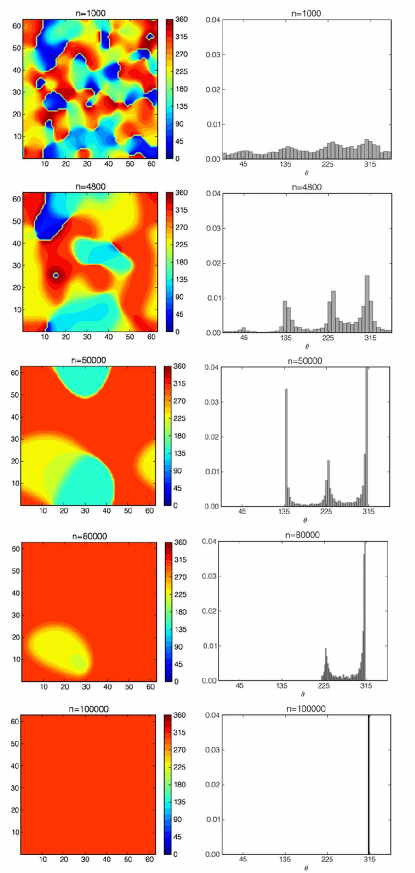
Figure 6: Run (c). Snapshots of $\theta$ (left panels) and corresponding histograms (right panels) at different steps $n$ during the simulation for a $64^{2}$ homogenous system with $\epsilon_{HB}=-1\times 10^{-4}$. At equilibrium the histogram is peaked at the value $\theta=7\pi/4$, which corresponds to one of the four minima of $V_{HB}$. The value of the attained minimum depends on the initial condition (here, same as in Fig. 5).

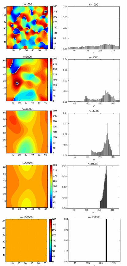
Figure 7: Run (d). Snapshots of $\theta$ (left panels) and corresponding histograms (right panels) at different steps $n$ during the simulation of a homogenous system of $64^{2}$ without DI’s. The final value of $\theta$ is random, and it depends on the initial condition (here, same as in Fig. 5).

IV.4 Heterogeneous scenario: hydrophobic effects

The above results pertain to a homogeneous scenario, with no hydrodynamic motion and away from solid boundaries. However, most important water-mediated phenomena take place in the proximity of solid boundaries, where heterogeneity plays a major role PhysTod; MELCH.

In view of future applications, it is therefore important to include these effects in our model. To this purpose, we have leveraged the LB capability to include non-ideal interactions (hydrophobic/hydrophilic) through density-dependent pseudo-potentials (Shan-Chen model, Eq. (7)). In particular, by adjusting the strength, $G_{b}$, of attractive fluid-fluid interactions in the bulk, we can generate an effective repulsion at walls, since a near-wall fluid layer would experience an attractive force from the second inner layer in the fluid and no force (or a smaller one) from the solid layer at the wall, thus resulting in an effective repulsion from the wall (hydrophobic effect). This strategy has been used by many authors in LB simulation of confined microfluids, and shown to give rise to density depletion layers near the wall (see LBmicro and references therein). Coupling the effect of these depletion layers with the density-dependent prefactor $\phi(\rho)$ of Eq. (10), permits to modulate the fluid structure as a function of distance from the solid walls.

For our tests, we have chosen a channel of size $N_{x}=32$ and $N_{y}=128$ with two layers of solid sites perpendicular to the $x$-direction, located at $x=2.5$ and $x=N_{x}-1.5$ (for computational reasons, we use two buffer layers and effective walls lie in between the second buffer and the first fluid layer). We used the half-way bounce back scheme for no-slip boundary conditions, i.e particles exiting the fluid domain are bounced backed into the fluid with the opposite velocity, along both normal and tangential directions. We set the parameter for the Shan-Chen interaction (see Eq. (7)) to $G_{b}=-3.8$, a value slightly below the critical threshold leading to liquid-vapor phase separation. We used the value $\varepsilon_{HB}=-0.1$ in $V_{HB}$. The initial condition was set to $\rho({\bf x})=\ln{2}$ everywhere within the channel. The density at the wall sites was fixed to $\rho_{\rm wall}=0.55<\ln{2}$ and we set $\rho_{\rm min}=\rho_{\rm wall}$. With these parameters, the maximum density (reached at the center of the channel, as illustrated in Fig. 8), was $\rho_{\rm max}=0.72$, corresponding to a density depletion ratio of about $25\%$. We first consider the static scenario (no net flow) with $\tau_{T}/\tau_{D}=10^{-6}$ and $\epsilon=0.001$.

The averaged density profile $\rho(x)=\frac{1}{N_{y}}\sum_{y=1}^{N_{y}}\rho(x,y)$ as a function of the distance from the wall is shown in Fig. 8 (top). From this figure, a depletion layer extending about $\delta=4\Delta x$ (4 lattice sites) away from the wall is well visible. The width of this layer is of the same order of magnitude of the interaction range, namely $\sqrt{2}\Delta x$ in the present nine speed lattice model.

To inspect the ordering effect, we have computed the correlation function of the $\theta$ domains, namely

$$C_{\theta}(x;r_{y})={<\theta(x,y+r_{y})\theta(x,y)>\over<\theta(x,y)^{2}>}$$ (27)

where the brackets stand for ensemble average over initial conditions and along the $y$-axis. The correlation function as a function of $r_{y}$, at various locations away from the wall, $x=4,8,10,16$ (in lattice units), is shown in Fig. 8 (bottom). Near the wall, correlations decay basically within one lattice site, because the strong effect of the torque dominates over diffusion effects, quenching the system around the minima of $V_{HB}$ closest to the initial value of $\theta$. On the other hand, at the center of the channel, correlations persist over larger distances, because diffusive effects lead to ordering within larger domains. The contour plot of the $\theta$-domains is shown in Fig. 9 (left panels), together with the corresponding histogram.

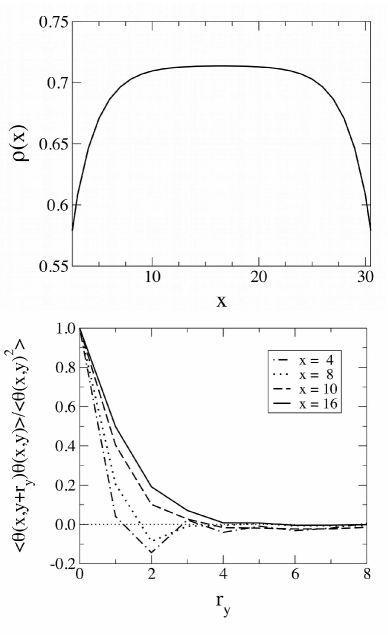
Figure 8: Density profile (top) as a function of the distance from the walls located at $x=2.5$ and $x=N_{x}-1.5$ and correlation function of $\theta$ (bottom) as a function of $r_{y}$ at various locations $x$, from close to the wall to the center of the channel.

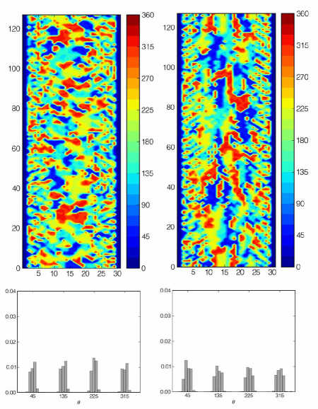
Figure 9: Left panels: Contour plot and corresponding histogram of the $\theta$ domains in a heterogeneous system. The histogram is nearly equi-distributed among the four degenerate minima of the HB potential. Right panels: Contour plot and corresponding histogram of the $\theta$ domains in a heterogeneous system with flow advection. The histogram is still nearly equally distributed among the four degenerate minima, but with an enhanced spreading due to advective motion.

IV.5 Flowing systems

In the Introduction, we have emphasized the crucial role played by hydrodynamic interactions in water transport phenomena under confinement MELCH. We have also highlighted the remarkable capability of LB methods to include hydrodynamic effects in the study of the dynamics of complex flows, including polar ones NELIDO; Cates, at virtually no extra computational cost. In this section, we provide just a qualitative example of such capability, leaving an in-depth analysis and applications to future publications. We consider the heterogeneous scenario discussed in the previous section, in the presence of a Poiseuille flow between the two confining walls. Specifically, $u_{x}=0$ and $u_{y}(x)=4U_{0}(x/W)(1-x/W)$, where $U_{0}$ is the centerline speed and $W$ the channel width. The relevant dimensionless parameter, measuring the strength of convection versus diffusion, is the Péclet number $Pe=U_{0}W/D_{p}$. With $\epsilon=0.001$, hence $D_{p}=0.001/3$, $W=32$ and $U_{0}=0.02$, we have $Pe\sim 2000$, indicating a strong dominance of advective effects over diffusive ones. However, advection still is three orders of magnitude slower than DI interactions, which therefore remain the dominant mechanism. Looking at the typical timescales, we have that $\tau_{T}/\tau_{D}=10^{-6}$ and we can estimate the ratio $\tau_{adv}/\tau_{D}$ as $\sim 1/Pe$. Note that the typical advection time $\tau_{adv}$ takes an intermediate value between the torque and diffusion times.

The main qualitative effect of advective motion, and particularly of the shear $s_{xy}=\partial u_{y}/\partial x\sim U_{0}/W$, is to promote mechanical deformation of the $\theta$ domains, as one can appreciate from Fig. 9 (right panels). This deformation is accompanied by a mild extra-mixing, as witnessed by the broadening of the $\theta$ histograms in the bottom panel of the same figure. This is in line with the qualitative idea of advection as an additional mixing mechanism, which, in the limit of high Péclet numbers, becomes correspondingly more effective than diffusion in competing with the ordering effect of directional interactions.

As stated above, a quantitative inspection of these complex phenomena will be left for future studies. Nevertheless, Fig. 9 conveys an idea of the kind of complexity that can be tackled by the water-like LB model presented in this work.

V Conclusion and Outlook

Summarizing, we have developed a mesoscopic lattice Boltzmann model for water-like fluids. By water-like, we imply that the fluid includes directional interactions (DI’s) mimicking (some) generic features of hydrogen-bonds, particularly the tendency to form ordered domains, with selected bond angles, against the action of thermal noise. The competition between the ordering effect of directional interactions against thermal disorder is shown to lead to the formation of complex patterns of the orientational order parameter, consisting of a disordered collection of ordered domains (i.e., in each domain the order parameter takes a uniform value). In addition, we have included non-ideal interactions which permit to realize heterogeneous density depletion layers near solid walls. By letting the DI’s carry an inverse density dependence, the model is able to incorporate a built-in correlation between ordered domains and low density regions, reflecting the idea of water as a denser liquid in the disordered state than in the ordered one.

The extension of our model to the three dimensional (3d) case does not present any conceptual barrier. The 3d water molecule would be represented by four bonding arms, arranged in a tetrahedral symmetry tetra2. This geometry requires two independent orientation angles for each lattice site. As far as the lattice is concerned, a possibility to accommodate the tetrahedral geometry is the standard cubic 15-speed lattice commonly used in 3d lattice Boltzmann simulations.

This paper sets a methodological starting basis for LB models of water-like fluids. A fully quantitative validation against microscopic models remains as a task for the future, warranting a separate investigation on its own. The model is expected to prove mostly valuable for the study of nanoscopic water flows with suspended molecules and/or charged ions, both in standalone HORBACH and/or multiscale scenarios DELGADO; multiscale.

VI Acknowledgements

Valuable exchange of information with I. Pagonabarraga, A. Scagliarini, F. Rao and N. González-Segredo is kindly acknowledged. We are grateful to A. Greiner for useful discussions. MV is supported by the Istituto Italiano di Tecnologia (IIT) under the SEED project grant No.259 SIMBEDD.