Phase separation in fluids exposed to spatially periodic external fields

Abstract

We consider the liquid-vapor type phase transition for fluids confined within spatially periodic external fields. For a fluid in $d=3$ dimensions, the periodic field induces an additional phase, characterized by large density modulations along the field direction. At the triple point, all three phases (modulated, vapor, and liquid) coexist. At temperatures slightly above the triple point and for low (high) values of the chemical potential, two-phase coexistence between the modulated phase and the vapor (liquid) is observed. We study this phenomenon using computer simulations and mean-field theory for the Ising model. The theory shows that, in order for the modulated phase to arise, the field wavelength must exceed a threshold value. We also find an extremely low tension of the interface between the modulated phase and the vapor/liquid phases. The tension is of the order $10^{-4}\,k_{B}T$ per squared lattice spacing, where $k_{B}$ is the Boltzmann constant, and $T$ the temperature. In order to detect such low tensions, a new simulation method is proposed. We also consider the case of $d=2$ dimensions. The modulated phase then does not survive, leading to a radically different phase diagram.

I Introduction

Liquid-vapor type phase transitions in fluids are profoundly affected by confinement (for a recent review see Ref. citeulike:3533972, ). Typical effects are the depression of critical temperatures fisher.nakanishi:1981 , changes in universality gennes:1984 , or entirely new phenomena altogether citeulike:7749811 ; citeulike:9633515 . The confinement of a fluid between two parallel surfaces is arguably the most simple example one could envision fisher.nakanishi:1981 . Already for this case the corresponding phase behavior is extremely rich, especially if the surfaces have different interactions with the fluid citeulike:9633515 ; virgiliis.vink.ea:2006 . With the advance of microcontact printing citeulike:9608754 , vapor deposition and grafting methods citeulike:9726164 , as well as photolithography citeulike:4014772 , the possibilities of tuning the surface-fluid interaction are essentially endless. In addition to surfaces, confinement in fluids may also be induced via external fields (for example, optical tweezers can be used to realize one-dimensional diffusion channels for colloidal particles in suspension citeulike:9609811 ). Hence, well-characterized geometries of ever increasing complexity can be generated, and the phase behavior of fluids confined within these is expected to become correspondingly richer.

With these developments in mind, this paper considers the fate of the liquid-vapor transition in a fluid confined within a static external field having periodic spatial oscillations in one direction. In $d=2$ dimensions, such a field might be realized using a stripe-patterned surface citeulike:4729899 ; citeulike:9258031 , while in $d=3$ dimensions, laser citeulike:9726153 or electric fields citeulike:5887157 ; citeulike:9726103 ; citeulike:9726113 could possibly be used. The case $d=3$ was first considered theoretically in Ref. citeulike:7530595, for a colloid-polymer mixture. The main finding was a new kind of phase transition, referred to as laser-induced condensation (LIC), which takes place provided the field wavelength is large enough. In the presence of the periodic field, one then observes a new third phase (in addition to the vapor and liquid phases) characterized by (i) an average density between that of the vapor and liquid phase, and (ii) featuring large density modulations along the field direction (because of the latter modulations we refer to this phase as the “zebra” phase in what follows). The presence of the zebra phase dramatically alters the liquid-vapor phase diagram: the critical point of the bulk transition is replaced by two new critical points and a triple point. At temperatures between the triple and critical points, vapor-zebra and liquid-zebra two-phase coexistence is observed (at low and high values of the chemical potential, respectively).

In a subsequent publication citeulike:9633508 the nature of the critical points was elucidated, and also the tensions $\gamma_{\rm vz}$ and $\gamma_{\rm lz}$ of, respectively, the vapor-zebra and liquid-zebra interfaces were calculated. The main observations were a critical behavior corresponding to effectively $d=2$ dimensions (i.e. one below the system dimension), and extremely low interfacial tensions. The latter were found, using density functional theory, to be at most $\gamma_{\rm vz}\sim\gamma_{\rm lz}\sim 10^{-5}~{}k_{B}T$ per projected particle area (with $k_{B}$ the Boltzmann constant, and $T$ the temperature). The accompanying simulations confirm that $\gamma_{\rm vz}$ and $\gamma_{\rm lz}$ must be extremely low, but no numerical values could be obtained (from the simulation data of Ref. citeulike:9633508, , interface tensions of exactly zero cannot be completely ruled out either).

In this paper, we revisit LIC using computer simulations and mean-field theory for the Ising model. Compared to a colloid-polymer mixture, computer simulations of the Ising model allows for much faster equilibration, such that larger system sizes can be reached. In addition, the underlying spin reversal symmetry of the Ising model makes the finite-size scaling analysis much more straight-forward. Of course, since the universality class of fluids is the Ising one, generic trends observed in the latter directly apply to fluids as well. We first consider LIC in $d=3$ dimensions. The corresponding phase diagram is calculated using both simulation and theory. In particular, we demonstrate how the phase diagram depends on the field wavelength and amplitude. Our next aim is to measure the interface tensions $\gamma_{\rm vz}$ and $\gamma_{\rm lz}$: it is important to confirm the density functional prediction that $\gamma_{\rm vz}$ and $\gamma_{\rm lz}$ are extremely low but finite. As it turns out, accurate measurements of such extremely low tensions are beyond the scope of “standard” methods citeulike:9039746 ; citeulike:9246548 , and so an alternative route is proposed. Finally, we consider LIC in $d=2$ dimensions. Since the critical behavior was shown to be of dimension $d-1$ citeulike:9633508 , we expect radical departures from the previously considered case $d=3$. Indeed, in $d=2$ dimensions, the two critical points do not survive, and an altogether different phase diagram is obtained.

II Model and Simulation method

We consider the Ising model on rectangular $L\times L\times D$ ($d=3$) and $L\times D$ ($d=2$) lattices with periodic boundary conditions in all directions. The system is exposed to a periodic external field $V_{\rm per}(z)$, with the $z$-axes parallel to edge $D$ of the lattice. To each lattice site $i$, a spin variable $s_{i}=\pm 1$ is attached. The energy of the system is given by

$$E=-J\sum_{\langle i,j\rangle}s_{i}s_{j}+H\sum_{i}s_{i}+\sum_{i}s_{i}V_{\rm per}(z_{i}),$$ (1)

where the first sum is over nearest neighbors, and the remaining sums over sites. The first term is the usual Ising pair interaction with coupling constant $J$ (we consider ferromagnetic interactions $J>0$ only). The second term is the interaction of the spins with a homogeneous external magnetic field of strength $H$. The last term represents the interaction with the periodic field, where $z_{i}$ is the $z$-coordinate of spin $i$. For the periodic external field we use a block wave of alternating sign

$$V_{\rm per}(z)=\begin{cases}-h&0<z\leq\lambda/2,\\ +h&\lambda/2<z\leq\lambda,\\ \end{cases}$$ (2)

with $h$ the field strength, and $\lambda$ the wavelength. Due to the discretization of the lattice we must choose $\lambda=2an_{1}$, with $a$ the lattice constant, and $n_{1}$ an integer. The use of periodic boundary conditions implies that the lattice edge $D=\lambda n_{2}$, with $n_{2}$ also an integer. In what follows, the lattice constant is the unit of length $a\equiv 1$. In addition, a factor of $1/k_{B}T$ is assumed to have been absorbed into the coupling constants $J$, $H$ and $h$ such that these quantities are dimensionless.

Monte Carlo simulations and mean-field theory are used to study the phase behavior of the above model. The key output of the simulations is the distribution $P(m)$, defined as the probability of observing the system in a state with magnetization $m=(1/N)\sum_{i}s_{i}$, with $N=DL^{d-1}$ the total number of lattice sites. We emphasize that $P(m)$ depends on all the model parameters introduced above, including the system size. To obtain $P(m)$ we use single spin-flip dynamics newman.barkema:1999 combined with successive umbrella sampling virnau.muller:2004 ; the latter scheme ensures that $P(m)$ is obtained over the entire range $-1\leq m\leq 1$, including those regions where $P(m)$ is very small. We also use histogram reweighting ferrenberg.swendsen:1988 to extrapolate data obtained for one set of values of the coupling constants to different (nearby) values.

III Results in $d=3$ dimensions

In this section we present results for the case $d=3$. We begin in Sec. III.1 with simulation results obtained for an external potential with strength $h=0.075$ and wavelength $\lambda=10$. Following this, in Sec. III.2, we present mean-field theory results for how the phase diagram varies as the parameters $h$ and $\lambda$ are varied.

III.1 Laser-induced condensation: phase diagram

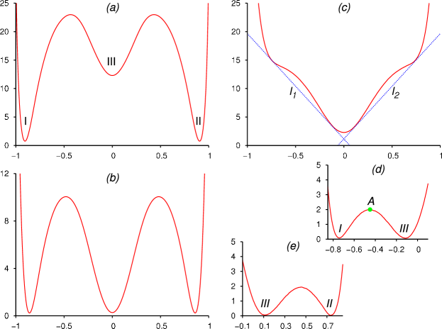
Figure 1: LIC in the $d=3$ Ising model; plotted in each of the graphs is the free energy $F(m)$ in units of $k_{B}T$ (vertical axes) versus the magnetization $m$ (horizontal axes). The free energy curves present actual simulation data obtained for system size $L=10$ and $D=\lambda$. (a) Free energy for $J>J_{\rm tr}$ and $H=0$, i.e. above the triple point. A coexistence between two phases, I and II, is observed. (b) Free energy for $J=J_{\rm tr}$ and $H=0$, i.e. exactly at the triple point; three-phase coexistence is observed. (c) Free energy measured between the triple and critical points, $J_{\rm cr}<J<J_{\rm tr}$, but still using $H=0$. We now observe two “common tangent” lines: $l_{1}$ and $l_{2}$. By choosing $H=\Delta_{1}$, where $\Delta_{1}$ is determined from the slope of $l_{1}$, coexistence between phases I and III can be induced (d). Similarly, from the slope of $l_{2}$, we obtain $H=\Delta_{2}$, at which phases II and III coexist (e).

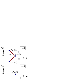
Figure 2: (a) Phase diagram of LIC for the $d=3$ Ising model. The phase diagram is a symmetric “pitchfork” featuring one triple point, and two critical points (indicated by dots). The lines correspond to first-order phase transitions (between phases I-II, I-III, and II-III). (b) LIC in $d=2$ dimensions. In this case, there is no phase III. The phase diagram features only a single line of first-order phase transitions terminating in a critical point.

To understand LIC in the Ising model it is best to consider the free energy $F(m)$ as function of the magnetization $m$. The latter is related to the magnetization probability distribution, $F(m)=-k_{B}T\ln P(m)$, to which we have direct access in our simulations. In Fig. 1(a), we show $F(m)$ for a high value of the coupling constant $J$ and $H=0$. The salient features are two global minima, at low and high values of $m$, reflecting a coexistence between two phases (I and II). We also observe a local minimum at $m=0$, corresponding to a phase III, but it is meta-stable. In (b), we plot $F(m)$ for a lower value of $J$ and $H=0$. We now observe three minima at equal height corresponding to a triple point, where all three phases coexist. Next, in (c), we show $F(m)$ for an even lower value of $J$, but still using $H=0$. There is now only one global minimum at $m=0$. However, by applying an appropriate homogeneous field $H=\Delta_{1}$, a coexistence between phase I and III is obtained (d). The value of $\Delta_{1}$ follows from the slope of the “common tangent” line $l_{1}$. Similarly, by applying a homogeneous field $H=\Delta_{2}$ (determined from the slope of line $l_{2}$), coexistence between phase II and III is obtained (e). Finally, at some critical value $J=J_{\rm cr,1}(J_{\rm cr,2})$, the I-III (II-III) coexistence line terminates, below which there is only one phase.

Fig. 1 is the analogue of LIC citeulike:7530595 in the Ising model, with phase I playing the role of vapor (v), phase II of the liquid (l), and phase III of the zebra (z) phase. Due to spin reversal symmetry, it holds that $H=0$ at the triple point $J=J_{\rm tr}$. Below the triple point, symmetry implies that $\Delta_{1}=-\Delta_{2}\equiv\Delta$ and $J_{\rm cr,1}=J_{\rm cr,2}\equiv J_{\rm cr}$. The resulting phase diagram is a symmetric pitchfork (Fig. 2(a)). The crucial difference with fluids (which typically lack spin reversal symmetry) is that the phase diagram is asymmetric in that case: $J_{\rm cr,1}\neq J_{\rm cr,2}$ and the fields (chemical potentials) $\Delta_{i}$ are not trivially related to each other citeulike:9633508 .

We emphasize that the free energy curves in Fig. 1 are obtained in simulations using $D=\lambda$. If one instead uses $D=\lambda n_{2}$ with integer $n_{2}>1$, one finds that $F(m)$ develops additional minima, as discussed in detail in Ref. citeulike:9633508, . These additional minima reflect meta-stable coexistence states and should not be confused with new phases. Hence, also when $D>\lambda$, the generic mechanism of LIC as shown in Fig. 1 still applies.

III.2 Stability of the zebra phase:
mean-field calculations

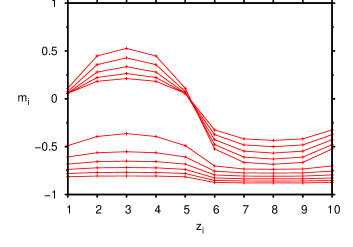
Figure 3: A sequence of magnetization profiles for varying $J$, going from $J=0.14$ (top) to $J=0.24$ (bottom), in increments of 0.01 obtained from the mean-field theory. For low values of $J$, one observes phase III, which is characterized by large modulations in the magnetization profile. For high values of $J$, phase II is observed, which is characterized by an overall low value of the magnetization and only small modulations. Note the discontinuous change in the profiles as the system crosses the II–III phase boundary (here at $J\approx 0.18-0.19$). The remaining parameters used in the figure are $H=0.03$, $h=0.075$ and $\lambda=10$.

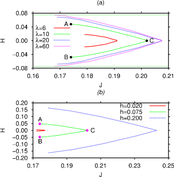
Figure 4: LIC phase diagrams for $d=3$ obtained using mean-field theory (for clarity only the transition lines between the zebra III phase and the I and II phases are shown). In (a) we show results for $h=0.075$ and various values of the field wavelength $\lambda$. In (b) we show results for $\lambda=10$ and various values of the field amplitude $h$.

In order to develop a qualitative understanding of how the LIC phase diagram of Fig. 2(a) depends on the external field wavelength $\lambda$ and amplitude $h$, we use the following simple mean-field (Bragg-Williams) approximation PlBi06 ; ChLu00 for the free energy $F$ of the system with Hamiltonian $E$, given in Eq. (1):

$$F=\sum_{i}\Bigg{[}k_{B}T\frac{1+m_{i}}{2}\ln\left(\frac{1+m_{i}}{2}\right)$$

$$+k_{B}T\frac{1-m_{i}}{2}\ln\left(\frac{1-m_{i}}{2}\right)$$

$$+Hm_{i}-m_{i}V_{\rm per}(z_{i})\Bigg{]}-J\sum_{\langle i,j\rangle}m_{i}m_{j},$$ (3)

where $m_{i}\equiv\langle s_{i}\rangle$ is the average magnetization at lattice site $i$. For a given external potential $V_{\rm per}(z)$, the average magnetization profile corresponds to the set $\{m_{1},m_{2},\cdots\}$ which minimize the free energy (3); i.e. are the solution to the set of equations $\partial F/\partial m_{i}=0$. This yields the following set of $i$ simultaneous equations:

$$\frac{k_{B}T}{2}\ln\left(\frac{1+m_{i}}{1-m_{i}}\right)+H-V_{\rm per}(z_{i})-J\sum^{\prime}_{j}m_{j}=0,$$ (4)

where $\sum^{\prime}_{j}$ denotes the sum over the 6 (in $d=3$) nearest neighbor lattice sites of site $i$. Because the external potential $V_{\rm per}(z)$ in Eq. (2), only varies in the $z$-direction, we have magnetization profiles that only vary in this one direction and so solving Eqs. (4) is straightforward. We do so using a simple (Picard) iterative numerical scheme. In Fig. 3 we show some example magnetization profiles calculated for various different values of $J$ as one crosses the transition line from phase II to the zebra phase III. We see a discontinuous change in the average magnetization in the system as one crosses the phase transition.

In Fig. 4(a) we show phase diagrams for various values of the field wavelength $\lambda$ and fixed field amplitude $h=0.075$ (the upper and lower horizontal lines correspond to $\pm h$, respectively). Note that for clarity we only display the I-III and II-III coexistence lines and do not display the I-II liquid-vapor coexistence line. For $\lambda=10$, the zebra critical points are marked $A$ and $B$, while point $C$ indicates the triple point. In the limit $\lambda\to\infty$, the critical points $A$ and $B$ shift toward $(J_{\rm cr,bulk},\pm h)$, respectively, where $J_{\rm cr,bulk}=1/6$ in the mean-field theory. As $\lambda\to\infty$, essentially two infinite systems are obtained: one inside a positive (homogeneous) external field $h$, and one inside a negative field $-h$. The value of $H$ at the respective critical point simply has to “cancel” this field. In the opposite limit $\lambda\to\lambda_{\rm min}=2$, we observe the loss of the zebra phase. In order for the zebra phase to survive, $\lambda/2$ must exceed the bulk correlation length which is the quantity that determines the distance over which the average density changes from one value to another. Indeed, for $\lambda=4$ and smaller, the critical points $A$ and $B$ can no longer be identified, and only point $C$ survives (which then no longer is a triple point, but a critical point, marking the end of the I-II coexistence region). When $\lambda=4$ and $h=0.075$ the mean-field critical point is at $J\approx 0.177$ and when $\lambda=2$ it is at $J\approx 0.169$. Recall that the mean-field bulk critical point (i.e. for $h=0$) is at $J_{\rm cr,bulk}=1/6\approx 0.167$.

In Fig. 4(b) we show phase diagrams for fixed $\lambda=10$ (chosen above the threshold such that the zebra phase survives) and various values of the field amplitude $h$. In the limit $h\to 0$, we observe that the points $A$, $B$ and $C$ all approach $(J_{\rm cr,bulk}=1/6,H=0)$, the critical point of the bulk system. When $h$ is very small, it is difficult to locate numerically the transition points. However, a threshold value of $h$ below which the zebra phase vanishes appears to be absent in this case (in contrast to the case as $\lambda$ is decreased). The effect of increasing $h$ is that the I-III and II-III transition lines open-up, with the transition points $A$, $B$ and $C$ shifting toward larger values of $J$. Note that the value of $H$ at the critical point is always less in magnitude than the value of $h$. When $h=0.02$, then the critical value $H_{\rm cr}\approx 0.005$; when $h=0.2$, then $H_{\rm cr}\approx 0.163$ and when $h=2$, then $H_{\rm cr}\approx 1.957$. We see from these that as $h$ becomes large, then $H_{\rm cr}\to h$.

III.3 Finite-size scaling analysis

We now continue with our simulation analysis using $\lambda=10$ and $h=0.075$. Finite-size scaling is used to locate the triple and critical points. We measure $P(m)$ for various values of $L$, keeping $D=\lambda$ fixed. We thus assume that correlations in the $z$-direction are “cut-off” by the periodic field, and so we do not need to scale in this direction (we return to this point shortly). The distribution $P(m)$ is always measured at $H=0$ and symmetrized by hand afterward such that $P(m)=P(-m)$, thereby imposing the spin reversal symmetry of the Ising model; subsequent histogram reweighting (in $J$ and $H$) is performed using the symmetrized distribution.

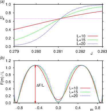
Figure 5: Finite-size scaling analysis to locate the LIC triple point for the $d=3$ Ising model. (a) Binder cumulant $U_{4}$ versus the coupling constant $J$ for various system sizes $L$. The curves strikingly intersect at $U_{4}=2/3$ (horizontal line) of a triple point; the value of $J$ at the intersection yields $J_{\rm tr}$. (b) The scaled free energy $F(m)/L$ precisely at the triple point, $J=J_{\rm tr}$, for various system sizes. Clearly visible are the three minima, corresponding to the coexisting phases, and a free energy barrier that increases linearly with $L$.

To determine $J_{\rm tr}$ we use $H=0$ and assume that, precisely at the triple point, the magnetization distribution $P(m)$ is a superposition of three (non-overlapping) Gaussian peaks, centered around $m=-m_{0}$, $m=0$, and $m=+m_{0}$, respectively. For such a triple-peaked distribution one may easily show that the Binder cumulant $U_{4}=2/3$, with the cumulant defined as

$$U_{4}\equiv\langle m^{2}\rangle^{2}/\langle m^{4}\rangle,\quad\langle m^{k}\rangle=\int_{-1}^{+1}m^{k}P(m)\,dm,$$ (5)

and where it is assumed that $P(m)$ is normalized. In Fig. 5(a), for the case when $h=0.075$ and $\lambda=10$ we plot $U_{4}$ versus $J$ for various system sizes $L$. The curves strikingly intersect at the expected “height” of a triple point, from which we conclude that $J_{\rm tr}\approx 0.2811$. Note that this exceeds $J_{\rm cr,bulk}\approx 0.2217$ of the critical point in the bulk ($h=0$) Ising model orkoulas.panagiotopoulos.ea:2000 , consistent with the general observation that confinement lowers transition temperatures. In Fig. 5(b), we plot the free energy $F(m)$ at the triple point for various system sizes. The curves clearly show the three minima of the coexisting phases. Note that the minima are shifted to zero, and that the vertical scale is divided by $L$. In this representation, the barrier $\Delta F/L$ (vertical arrow) is approximately constant. Hence, at the triple point, we observe a free energy barrier that increases linearly with the system size $\Delta F\propto L$. This implies that the general shape of $F(m)$, i.e. featuring three minima, persists in the thermodynamic limit $L\to\infty$, and thus reflects a genuine triple point (see also Ref. citeulike:3908342, where these ideas were first applied to first-order phase transitions).

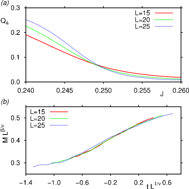
Figure 6: Finite-size scaling analysis to locate the LIC critical point for the $d=3$ Ising model. (a) Cumulant $Q_{4}$ versus the coupling constant $J$ for various system sizes $L$; the intersection yields $J=J_{\rm cr}$. (b) Scaling plot of the order parameter $M$ where $t=J/J_{\rm cr}-1$; by using $J_{\rm cr}\approx 0.2531$ and $d=2$ Ising values for the critical exponents $\beta,\nu$ the data for different $L$ collapse onto a single master curve.

For values of $J$ between the triple and critical points, coexistence with the zebra phase (phase III) is observed at appropriate values $H=\pm\Delta$ of the external magnetic field. To locate $J_{\rm cr}$ we perform the same cumulant analysis as in our previous work citeulike:9633508 . For a given value of $J$, $\langle m\rangle$ and $U_{4}$ are measured as function of $H$ (due to symmetry, only $H\geq 0$ needs to be considered). One then uses these data to construct a graph of $U_{4}$ versus $\langle m\rangle$ (which thus is parametrized by $H$). The resulting curve reveals a maximum, corresponding to $H=\Delta$, enveloped by two minima kim.fisher:2004 . The average value of the cumulant at the minima equals $Q_{4}$. In Fig. 6(a), we plot $Q_{4}$ versus $J$ for different $L$; from the intersection point we conclude that $J_{\rm cr}\approx 0.2531$ (the corresponding critical field $\Delta_{\rm cr}\approx 0.017$). The difference $M$ in the magnetizations $\langle m\rangle$ at the minima yields the order parameter. The latter is analyzed in the finite-size scaling plot newman.barkema:1999 ; binder.heermann:2002 of Fig. 6(b). The key result is that, by using the $d=2$ Ising values for the critical exponents ($\beta=1/8,\nu=1$) the data for different $L$ collapse. The critical points of LIC in $d=3$ dimensions thus remain in the universality class of the Ising model, but of reduced dimensionality $d-1$. We believe that colloid-polymer mixtures should ultimately yield the same exponents, but that their complexity still prevents efficient simulations of large enough systems to explicitly see this citeulike:9633508 .

III.4 Measurement of ultra-low surface tension

We now consider the regime between the triple and critical points using $H=\pm\Delta$. The free energy then schematically resembles Fig. 1(d,e), corresponding to I-III and II-III phase coexistence, respectively. Hence, there will be interfaces present, and our aim is to measure the corresponding interface tension $\gamma$ (due to symmetry it holds that $\gamma_{I,III}=\gamma_{II,III}\equiv\gamma$, of course). Following density functional calculations citeulike:9633508 , $\gamma$ is expected to be extremely low. In principle, for liquid-vapor transitions, the corresponding interface tension $\gamma_{\rm lv}$ can be accurately determined from the free energy using an idea of Binder binder:1982 . In our previous work citeulike:9633508 , we discussed how this approach may be generalized to LIC, but it was clear that present computer power is not sufficient to reach the system sizes required for this method to work. Hence, we propose a different method.

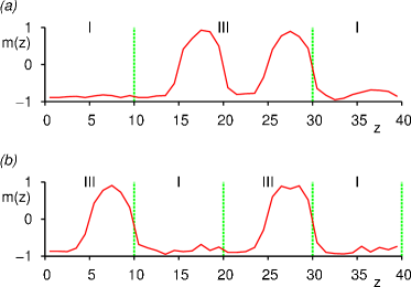
Figure 7: Instantaneous magnetization profiles $m(z)$ obtained for $J=0.275$, $L=14$, and fixed overall magnetization $m=-0.426$. In (a) we observe a coexistence between two domains, while in (b) a coexistence between four domains is seen. The vertical lines indicate the approximate locations of the interfaces. By counting how often the arrangements (a) and (b) occur during a long simulation run, the interface tension can be determined, see Eq. (6).

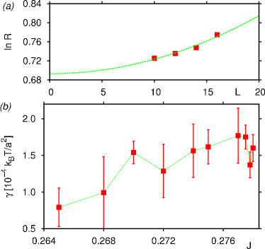
Figure 8: (a) Variation of $\ln R$ with system size $L$ for $J=0.275$; symbols are simulation data, the curve is a fit to Eq. (6). Note that the data are consistent with $\lim_{L\to 0}\ln R=\ln 2$ of the entropy difference. (b) The interfacial tension $\gamma$, in units of $k_{B}T$ per squared lattice spacing, as a function of $J$. In agreement with theoretical expectations citeulike:9633508 , $\gamma$ is extremely low and decreases as $J\to J_{\rm cr}$.

The key observation is that the periodic field $V_{\rm per}(z)$ suppresses interface fluctuations (capillary waves) in the $z$-direction: even though $\gamma$ is very low, the I-III and II-III interfaces are sharp. This is in contrast to conventional liquid-vapor interfaces which, at low interface tension, are extremely broad vink.horbach.ea:2004*b ; aarts.schmidt.ea:2004 . The fact that the interfaces remain sharp is the property we exploit to extract $\gamma$. To this end, we consider a simulation box with edge $D=4\lambda$. In Fig. 7, we show instantaneous magnetization profiles $m(z)$ obtained for two equilibrated samples at fixed overall magnetization $m$. The value of $m$ must be chosen such that half the system is occupied by phase I, and the remainder by phase III, which can be obtained from the local maximum in the free energy (point “A” in Fig. 1(d)).

Since the interfaces are essentially flat, one can easily identify where the phases are located. In Fig. 7(a), we see one large domain of phase I (characterized by a low overall magnetization) coexisting with one large domain of phase III (characterized by large modulations in the magnetization). Hence, two I-III interfaces are present (recall that periodic boundaries are used). In Fig. 7(b), we again observe I-III phase coexistence, but this time the phases are arranged such that four I-III interfaces are present. In equilibrium, arrangement (a) is preferred since it has the smallest interface area: $2L^{2}$ versus $4L^{2}$, with $L$ the lateral box size. However, for finite $L$, arrangement (b) is also frequently observed, since $\gamma$ is small. In fact, from the ratio of counts $R$, the interface tension can be determined

$$\ln R=2\gamma L^{2}+\Delta S,\quad R\equiv n_{a}/n_{b},$$ (6)

where $n_{i}$ denotes the number of times arrangement $i=(a,b)$ was seen during a very long simulation run (note that this simulation must be performed at fixed $m$ chosen to yield equal volumes of both phases). The “offset” $\Delta S$ reflects the combinatorial and translational entropy difference between the arrangements. The former is zero since there are as many ways to distribute the phases as in (a), as there are for (b). However, there is additional translational entropy for arrangement (a) since the domains are twice as large (we thus expect $\Delta S=\ln 2\approx 0.69$).

To simulate at fixed $m$ we use Kawasaki dynamics: two spins of opposite sign are randomly selected and flipped, and the resulting spin configuration is accepted with the Metropolis criterion newman.barkema:1999 . To facilitate frequent transitions between arrangements (a) and (b) of Fig. 7, we also use a collective Monte Carlo move. To this end, we introduce the block domain $B_{i}$, which contains all spins whose $z$-coordinate is between $\lambda b_{i}/2<z\leq\lambda(b_{i}/2+1)$, with $b_{i}$ an integer (periodic boundary conditions must be applied). In the collective move, two block domains, $B_{1}$ and $B_{2}$, are randomly selected with the constraint that $|b_{1}-b_{2}|>0$ and even. The domains are then swapped, and the resulting spin configuration is accepted with the Metropolis criterion (in our simulations, Kawasaki and collective moves are attempted in a ratio $1:0.03$, respectively).

To test our approach we consider $0.264<J<0.278$, which is between the triple and critical points. We use $m=-0.426$ for this is the value where phases I and III were seen to occupy equal volumes. In Fig. 8(a), we plot $\ln R$ versus $L$ for $J=0.275$; the data are indeed well described by Eq. (6), and by fitting $\gamma$ can be estimated. In Fig. 8(b), we plot the corresponding estimates of $\gamma$ versus $J$. Despite the admittedly rather large statistical uncertainty, our data confirm that the tension is extremely low, and that it decreases as $J$ is lowered; both these observations are in qualitative agreement with theoretical predictions citeulike:9633508 .

III.5 Correlations in the field direction

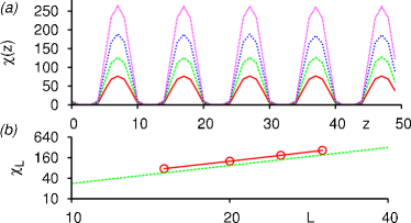
Figure 9: Investigation of the critical behavior using a simulation box with $D=5\lambda$; the simulations are performed at fixed magnetization $m=-0.426$ and $J=J_{\rm cr}$. (a) The susceptibility profiles $\chi(z)$ for $L=15,20,25,30$ (from bottom to top). The key point to note from this figure is that $\chi(z)$ diverges with $L$ only at special values $z=z_{\rm cr}$. (b) Finite-size scaling analysis of the average peak height $\chi_{L}$ of the susceptibility profiles. We plot is $\chi_{L}$ versus $L$ on double-logarithmic scales. The dashed line corresponds to a power-law with exponent $\gamma/\nu=7/4$ of the $d=2$ Ising model.

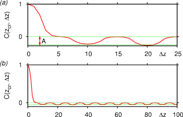
Figure 10: The correlation function $C(z_{\rm cr},\Delta z)$ in the critical regime. We show results for $D=5\lambda,\,L=30$ (a), and $D=20\lambda,\,L=8$ (b). The vertical arrow in (a) marks the amplitude $A$ of the anti-correlations, which conforms to Eq. (8).

In the finite-size scaling analysis of Section III.3 we varied $L$ keeping $D=\lambda$ fixed. We thus assumed the correlations in the field direction to be short-ranged: critical correlations only develop in the lateral $L$ directions, but not in the direction $D$ along the field, such that the resulting critical behavior is effectively two-dimensional (and belonging to the $d=2$ Ising universality class). To verify this assumption we now consider the critical regime using a larger value $D=5\lambda$. We perform simulations at $J=J_{\rm cr}$ and fixed $m=-0.426$ (the latter corresponds to the average magnetization at the critical point). To simulate at fixed $m$ we use Kawasaki dynamics and collective moves (as in the previous section). However, for the collective moves, the block domain $B_{i}$ was taken to be a single lattice layer, containing those spins whose $z$-coordinate equals $z_{i}$ (at criticality, this choice yields a higher accept rate). A pair of layers is chosen randomly and swapped, with the constraint that the sign of $V_{\rm per}(z)$ in the layers is the same, and accepted with the Metropolis criterion.

In Fig. 9(a), we plot the susceptibility profile $\chi(z)=L^{2}\left(\langle m(z)^{2}\rangle-\langle m(z)\rangle^{2}\right)$ for various values of $L$. The susceptibility diverges with $L$ only at selected values $z=z_{\rm cr}$, which “repeat” with the same period as the field. The critical behavior is thus spatially confined to those $L\times L$ slabs for which the corresponding $z$-coordinate equals one of the $z_{\rm cr}$. To determine the universality class we compare the average peak heights $\chi_{L}$ of the susceptibility profiles to the finite-size scaling prediction $\chi_{L}\propto L^{\gamma/\nu}$, with $\gamma$ the susceptibility critical exponent. This result is shown in Fig. 9(b), and the $d=2$ Ising value $\gamma/\nu=7/4$ is strikingly confirmed. Hence, the observed universality class does not depend on the value of $D$ used in the scaling analysis, which a posteriori provides the justification for the approach of Section III.3.

Next, we ask whether correlations exist between critical slabs. To this end, we introduce the pair correlation function

$$C(z_{1},\Delta z)\propto\\ \langle m(z_{1})\,m(z_{1}+\Delta z)\rangle-\langle m(z_{1})\rangle\langle m(z_{1}+\Delta z)\rangle,$$ (7)

measured between the slab at $z=z_{1}$ and $z=z_{1}+\Delta z$, respectively. We choose $z_{1}$ to coincide with one of the critical slabs, and we normalize such that $C(z_{1},0)\equiv 1$. In Fig. 10, we show the correlation function for a system with $D=5\lambda$ (a), and for $D=20\lambda$ (b). We find that the slabs at $\Delta z=n\lambda$ with integer $n>0$ are anti-correlated from the (critical) slab at $n=0$. Moreover, the amplitude $A$ of the anti-correlations is independent of $\Delta z$, but it decreases with $D$. In fact, an almost perfect “lever rule” is observed

$$A=\lambda/(D-\lambda).$$ (8)

That is: if there happens to be an excess magnetization in one of the critical slabs, the remaining critical slabs respond by assuming a lower magnetization, in a manner such that the excess magnetization is shared equally on average. In the limit $D\to\infty$, the amplitude $A$ of the correlations becomes zero, consistent with our assumption that long-ranged correlations in the field direction are absent. We also point out that the correlations in Fig. 10 are very different from critical correlations; the latter decay as power laws, $\lim_{\Delta z\to\infty}C(z_{\rm cr},\Delta z)\propto 1/\Delta z^{\eta}$ with critical exponent $\eta$, for which we see no evidence in our data. In fact, the anti-type correlations of Fig. 10 are also observed in the non-critical regime of the phase diagram (explicit checks were performed for $J=0.27$ using $m=-0.82$ and $m=-0.04$, corresponding to a pure phase I and phase III, respectively).

IV Results in $d=2$ dimensions

We now consider LIC in $d=2$ dimensions. The simulations are performed on $L\times D$ periodic lattices, with the field $V_{\rm per}(z)$ again propagating along edge $D$ of the lattice. In what follows, the field wavelength $\lambda=8$ with strength $h=0.1495$.

IV.1 Phase diagram and scaling analysis

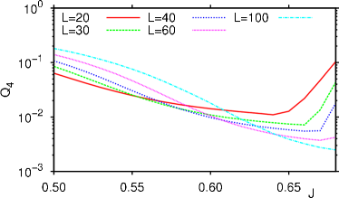
Figure 11: The analogue of Fig. 6(a) but for the case $d=2$. Note the logarithmic vertical scale. The data are obtained using fixed $D=\lambda$. The key thing to note from this figure is that the curves for different $L$ do not intersect at a single point, implying the absence of a critical point. This, in turn, is consistent with $d=1$ Ising universality.

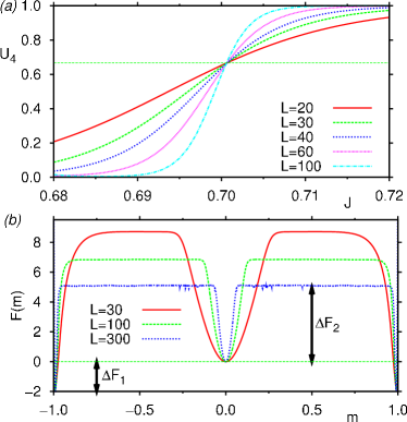
Figure 12: The analogue of Fig. 5 but for the case $d=2$. The main difference is that we now observe a critical point, as opposed to a triple point. (a) The Binder cumulant as function of $J$ for $H=0$ and different system sizes $L$. The curves for different $L$ intersect from which we might conclude that a phase transition takes place. However, we display in (b) the scaling with $L$ of the free energy $F(m)$ at the cumulant intersection, with $F(m=0)$ shifted to zero, where we see that the depth of the central minimum $\Delta F_{2}\to 0$ as $L$ increases, while the depth $\Delta F_{1}$ of the outer minima appears to be independent of $L$. This type of scaling is consistent with a critical point citeulike:3908342 .

We first determine whether the LIC critical points occur in $d=2$ dimensions also. Since the critical behavior was shown to resemble that of a reduced dimension $d-1$, we now expect the universality class of the $d=1$ Ising model. As is well known, the latter model does not feature a critical point. In Fig. 11, we repeat the cumulant analysis of Fig. 6(a). In line with the $d=1$ Ising model, we do not observe an intersection point, confirming the absence of a critical point. While for small $L$ the curves somewhat intersect, the intersections for larger $L$ systematically shift toward larger values of $J$. Hence, in $d=2$ dimensions, there is no LIC critical behavior.

Next, we investigate the fate of the triple point, using the same analysis as in Fig. 5. We collect data for fixed $H=0$ and $D=\lambda$, while $J$ and $L$ are varied. In Fig. 12(a), we plot the Binder cumulant $U_{4}$ versus $J$ for different system sizes $L$. Consistent with a triple point, we observe a sharp intersection, with the value of the cumulant at the intersection very close to $U_{4}=2/3$ of a triple-peaked distribution. However, the corresponding free energy is not consistent with a triple point, see Fig. 12(b), where $F(m)$ is plotted for three different system sizes; note that we plot $F(m)$ with the central ($m=0$) minimum shifted to zero. While $F(m)$ clearly reveals three minima, the central minimum does not survive in the thermodynamic limit. This can be seen from the corresponding “depth”, marked $\Delta F_{2}$ in the figure, which decreases with $L$. In the limit $L\to\infty$, we have $\Delta F_{2}\to 0$, and only the outer minima survive, whose corresponding depths then equal $\Delta F_{1}$. The observation in Fig. 12(b) that $\Delta F_{1}$ is independent of system size is characteristic of a continuous transition citeulike:3908342 . Hence, for LIC in $d=2$ dimensions, the triple point is destroyed, and replaced by a critical point, in this case at $J_{\rm cr}\approx 0.701$ (as expected, this exceeds $J_{\rm cr,bulk}=\ln(1+\sqrt{2})/2$ of the bulk $d=2$ Ising model). The LIC phase diagram in $d=2$ dimensions is thus radically different from $d=3$. Instead of a “pitchfork” topology, we now have a single line of first-order phase transitions terminating in a critical point (Fig. 2(b)).

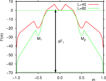
Figure 13: Free energy $F(m)$ for $d=2$ and $J=0.8>J_{\rm cr}$; the data are obtained using $D=2\lambda$, $H=0$, and two values of $L$ as indicated. The key thing to note from this figure is that the free energy barrier $\Delta F_{1}$ increases with $L$, indicating a first-order phase transition citeulike:3908342 . Note also the spurious minima $M_{1}$ and $M_{2}$: these reflect meta-stable coexistence states citeulike:9633508 whose role in the thermodynamic limit is negligible.

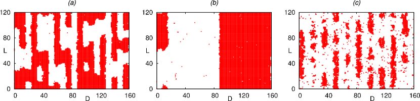
Figure 14: Computer generated snapshots obtained using $D=10\lambda$ and $L=120$; white regions correspond to “spin-up”. The snapshots in (a) and (b) are obtained for $J=0.8$ and $m=0$ and show “early time” and “late time” snapshots, respectively (the simulation was started with a random spin configuration). Since $J>J_{\rm cr}$ we observe coarsening of domains (a) until two large domains have formed (b). In (c), we show a snapshot for the case when $J=0.5<J_{\rm cr}$ and $m=0.52$. In this situation, domains do not coarsen with time, but remain finite in size, reminiscent of the $d=1$ Ising model.

We still find that, for $J>J_{\rm cr}$, the transition is first-order. In Fig. 13, we plot the free energy $F(m)$ for $J=0.8,\,H=0$ using system sizes $L=40,80$ and $D=2\lambda$. The free energy curves are again shifted such that $F(m=0)=0$. While for the smaller system the minimum at $m=0$ is still visible, it has vanished in the larger system. In addition, the barrier $\Delta F_{1}$ now increases profoundly with $L$, consistent with a first-order transition citeulike:3908342 . Note also the pronounced flat region in $F(m)$ around $m\sim 0$ for the larger system: this indicates two-phase coexistence with negligible interactions between the interfaces citeulike:7237424 . When a simulation is performed in this regime starting from a random initial spin configuration, the system phase separates to form structures that are strongly affected by the external potential; see Fig. 14(a). However, when the system is fully equilibrated at a “later time”, snapshots show the system containing two coexisting domains of phases I and II; see Fig. 14(b). In a box with periodic boundaries, the domains arrange themselves as two slabs since this minimizes the total interface length.

IV.2 Rounding effects

Even though the “zebra” phase (phase III), does not survive in the thermodynamic limit in $d=2$, we still see remnants of this phase in systems of finite size. If one simulates at $J<J_{\rm cr}$ using an appropriate external field $H$, one finds that in finite systems $F(m)$ can still be cast into the forms of Fig. 1(d,e). Inspection of simulation snapshots then reveals a condensation of droplets onto stripes oriented perpendicular to the field direction (Fig. 14(c)). However, the droplet size remains finite in this case, owing to the fact that the $d=1$ Ising model at finite temperature does not support a finite magnetization. Similar finite-size effects occur in colloid-polymer mixtures confined to cylindrical pores, which also belong to the universality class of the $d=1$ Ising model citeulike:7678249 ; citeulike:8132587 .

V Summary

In this work, we considered the phase behavior of the Ising model exposed to a static periodic field. In $d=3$ dimensions, we obtain a phase diagram analogous to laser-induced condensation observed in fluids undergoing bulk liquid-vapor type transitions. That is, a new phase arises (the “zebra” phase) and the critical point of the bulk model is replaced by two new critical points, and a triple point. The main difference compared with fluids is that, due to spin reversal symmetry, the corresponding phase diagram for the Ising model features a symmetry line. The analysis of the present work complements earlier works on laser-induced condensation citeulike:7530595 ; citeulike:9633508 in that (i) a detailed study of finite-size effects at the triple point was presented, (ii) a simple mean-field theory was used to elucidate in a qualitative manner how the $d=3$ phase transitions depend on the parameters in the external potential, (iii) a method was presented to measure the extremely low tension of interfaces with the zebra phase, and (iv) the nature of correlations along the field direction was further clarified.

We additionally considered the fate of laser-induced condensation in $d=2$ dimensions. In this case, we find that the zebra phase does not survive in the thermodynamic limit, and the corresponding phase diagram features just a single critical point. This critical point occurs at a temperature below the critical temperature of the pure $d=2$ Ising model. The universality class of the critical point still needs to be determined. The analysis of the free energy in Fig. 12(b) only indicates a critical transition, since the barrier $\Delta F_{1}$ is $L$-independent, but no information regarding critical exponents could be obtained. The practical problem here is that, in computer simulations, we are still restricted to system sizes that span only a few field wavelengths. We should also mention that the mean-field theory used in Sec. III B predicts very similar results in $d=2$ as it does in $d=3$ and is therefore not reliable when applied in $d=2$.

Even though our results were obtained for the relatively simple Ising model, the generic features of the observed phase behavior should also apply to real fluids. In particular the experimental realization in $d=2$ dimensions should be feasible using a stripe-patterned substrate. At moderate temperatures, the condensation of finite-sized droplets should be observable, while at low temperatures a macroscopic demixing should occur (c.f. Fig. 14).

- (1) K. Binder, J. Horbach, R. L. C. Vink, and A. De Virgiliis, Soft Matter 4, 1555 (2008)
- (2) M. E. Fisher and H. Nakanishi, J. Chem. Phys. 75, 5857 (1981)
- (3) P. G. De Gennes, J. Phys. Chem. 88, 6469 (1984)
- (4) A. Valencia, M. Brinkmann, and R. Lipowsky, Langmuir 17, 3390 (2001)
- (5) A. O. Parry and R. Evans, Phys. Rev. Lett. 64, 439 (1990)
- (6) D. A. Virgiliis, R. L. C. Vink, J. Horbach, and K. Binder, EPL 77, 60002 (2007)
- (7) J. Drelich, J. D. Miller, A. Kumar, and G. M. Whitesides, Colloids and Surfaces A: Physicochemical and Engineering Aspects 93, 1 (1994)
- (8) S. Minko, in: M. Stamm (Ed.), Polymer Surfaces and Interfaces, chap. 11, 215–234 (Springer Berlin Heidelberg, Berlin, Heidelberg, 2008)
- (9) R. Wang, K. Hashimoto, A. Fujishima, M. Chikuni, E. Kojima, A. Kitamura, M. Shimohigoshi, and T. Watanabe, Nature 388, 431 (1997)
- (10) C. Lutz, M. Kollmann, P. Leiderer, and C. Bechinger, J. Phys.: Condens. Matter 16, S4075 (2004)
- (11) H. Gau, S. Herminghaus, P. Lenz, and R. Lipowsky, Science 283, 46 (1999)
- (12) M. Tröndle, O. Zvyagolskaya, A. Gambassi, D. Vogt, L. Harnau, C. Bechinger, and S. Dietrich, Mol. Phys. 109, 1169 (2011)
- (13) H. von Grünberg and J. Baumgartl, Phys. Rev. E 75 (2007)
- (14) Y. Tsori, F. Tournilhac, and L. Leibler, Nature 430, 544 (2004)
- (15) Y. Tsori, Macromolecules 40, 1698 (2007)
- (16) T. L. Morkved, M. Lu, A. M. Urbas, E. E. Ehrichs, H. M. Jaeger, P. Mansky, and T. P. Russell, Science 273, 931 (1996)
- (17) I. O. Götze, J. M. Brader, M. Schmidt, and H. Löwen, Mol. Phys. 101, 1651 (2003)
- (18) R. L. C. Vink, T. Neuhaus, and H. Löwen, J. Chem. Phys. 134, 204907 (2011)
- (19) F. Varnik, J. Baschnagel, and K. Binder, J. Chem. Phys. 113, 4444 (2000)
- (20) K. Binder, B. Block, S. K. Das, P. Virnau, and D. Winter, J. Stat. Phys. in press (2011)
- (21) M. E. J. Newman and G. T. Barkema, Monte Carlo Methods in Statistical Physics (Clarendon Press, Oxford, 1999)
- (22) P. Virnau and M. Müller, J. Chem. Phys. 120, 10925 (2004)
- (23) A. M. Ferrenberg and R. H. Swendsen, Phys. Rev. Lett. 61, 2635 (1988)
- (24) M. Plischke and B. Bergersen, Equilibrium Statistical Physics, 3rd edition (World Scientific, Singapore, 2006)
- (25) P. M. Chaikin and T. C. Lubensky, Principles of Condensed Matter Physics (Cambridge University Press, Cambridge, 2000)
- (26) G. Orkoulas, A. Z. Panagiotopoulos, and M. E. Fisher, Phys. Rev. E 61, 5930 (2000)
- (27) J. Lee and J. M. Kosterlitz, Phys. Rev. B 43, 3265 (1991)
- (28) Y. C. Kim and M. E. Fisher, Comput. Phys. Commun. 169, 295 (2005)
- (29) K. Binder and D. W. Heermann, Monte Carlo Simulation in Statistical Physics: An Introduction (Springer, Berlin, Germany, 2002)
- (30) K. Binder, Phys. Rev. A 25, 1699 (1982)
- (31) R. L. C. Vink, J. Horbach, and K. Binder, J. Chem. Phys. 122, 134905 (2005)
- (32) D. G. Aarts, M. Schmidt, and H. N. Lekkerkerker, Science 304, 847 (2004)
- (33) B. Grossmann and M. L. Laursen, Nucl. Phys. B 408, 637 (1993)
- (34) D. Wilms, A. Winkler, P. Virnau, and K. Binder, Phys. Rev. Lett. 105, 045701 (2010)
- (35) A. Winkler, D. Wilms, P. Virnau, and K. Binder, J. Chem. Phys. 133, 164702 (2010)