Polarimetric Imaging of Sgr A* in its Flaring State

Abstract

The Galaxy’s supermassive black hole, Sgr A*, produces an outburst of infrared radiation about once every 6 hours, sometimes accompanied by an even more energetic flurry of X-rays. It is rather clear now that the NIR photons are produced by nonthermal synchrotron processes, but we still don’t completely understand where or why these flares originate, nor exactly how the X-rays are emitted. Circumstantial evidence suggests that the power-law electrons radiating the infrared light may be partially cooled, allowing for the possibility that their distribution should be more accurately described by a broken power law with a (“cooling break”) transition frequency. In addition, the emission region (energized by an as yet unidentified instability) appears to be rather compact, possibly restricted to the inner edge of the accretion disk. In that case, the X-ray outburst may itself be due to synchrotron processes by the most energetic particles in this population. In this paper, we examine several key features of this proposal, producing relativistically correct polarimetric images of Sgr A*’s NIR and X-ray flare emission, in order to determine (1) whether the measured NIR polarization fraction is consistent with this geometry, and (2) whether the predicted X-ray to NIR peak fluxes are confirmed by the currently available multi-wavelength observations. We also calculate the X-ray polarization fraction and position angle (relative to that of the NIR photons) in anticipation of such measurements in the coming years. We show that whereas the polarization fraction and position angle of the X-rays are similar to those of the NIR component for synchrotron-cooled emission, these quantities are measurably different when the X-rays emerge from a scattering medium. It is clear, therefore, that the development of X-ray polarimetry will represent a major new tool for studying the spacetime near supermassive black holes.

1 Introduction

Sagittarius A* (Sgr A*) is the radiative manisfestation of our galactic supermassive black hole. Discovered almost four decades ago (Balik & Brown 1974), this intriguing radio source has been well studied at all wavelengths, generating interest among both theorists and observers (see Melia 2007 for a comprehensive review). A significant development with Sgr A* occurred in 2001, with the discovery of bright X-ray flares emanating from its vicinity (Baganoff et al. 2001). Lasting anywhere from 40 minutes to over 3 hours, these events are associated with enhanced X-ray emission, 30–200 times greater than that of its quiescent state.

In the intervening years, many more X-ray flares have been observed by both Chandra and XMM-Newton, and analyzed extensively (see, e.g., Goldwurm et al. 2003, Porquet et al. 2003, Bélanger et al 2005, Porquet et al. 2008). Among the many intriguing features characterizing these events are temporal substructures as short as 200 s, indicating that the physical processes responsible for the outbursts occur within a mere 10–20 Schwarzschild radii of a $\sim 4\times 10^{6}\;M_{\odot}$ black hole (Schödel et al. 2002, Ghez et al. 2003).

Flaring events in Sgr A* have also been detected in the NIR (Genzel et al. 2003) and even at mm and sub-mm wavelengths (see, e.g., Zhao et al. 2004, Trap et al. 2011). At least in the infrared, the flare spectra appear to be power laws with variable linear polarization, suggesting optically thin synchrotron emission as the likely mechanism producing the excess flux. But though the observational profile of these bursts continues to be refined, in tandem with significant theoretical discourse and modeling, we still don’t completely understand where or why these flares originate, nor exactly how the X-rays are produced, or even if the variable mm and sub-mm emission is really indicative of the flares’ spectral extension into the radio domain. One thing is certain, however—that no significant progress is likely to occur without multiwavelength observations and a broadband approach to the data analysis and modeling. For this reason, several groups have systematically organized large simultaneous observational campaigns, utilizing both ground-based and orbital platforms (see, e.g., Bélanger et al. 2004, 2006, Yusef-Zadeh et al. 2006, Marrone et al. 2008, Yusef-Zadeh et al. 2009, Dodds-Eden et al. 2009, Kunneriath et al. 2010, Trap et al. 2011).

The key results emerging from these (and other similar) studies are as follows (see Dodds-Eden et al. 2009 for a more comprehensive compilation): (1) IR/NIR flares occur more frequently than X-ray flares, typically $\sim 4$ times per day, compared with roughly 1 per day for the latter; (2) consequently, every X-ray flare appears to be associated with an NIR flare, but not every NIR event is correlated with an X-ray flare; additionally, (3) though X-ray and NIR flares occur simultaneously, with no significant delay, the former are typically shorter in duration; (4) polarimetric measurements in the NIR show that the source is significantly polarized (by as much as $\sim 12\%-25\%$; see Eckart et al. 2006, Nishiyama et al. 2009; (5) the brightest flares have a constant spectral index $\alpha\sim 0.6$ between 3.8 and 1.6 $\mu$m, where the flux is given as $F_{\nu}\propto\nu^{-\alpha}$ (see, e.g., Hornstein et al. 2007). At lower intensities, there may also be a possible trend of spectral index with flux, though this is still in dispute.

Additional results emerge when we include observations at longer wavelengths, but our focus in this Letter will be on the NIR and X-ray emission, so we will defer the more complete discussion to a subsequent paper. As we shall see, three of the critical questions that must be resolved for a complete understanding of the flare phenomenon in Sgr A* (at least in the NIR/X-ray) are (1) how are the X-rays produced? (2) how do we understand Sgr A*’s polarized NIR flare emission? and (3) can we predict the associated polarization fraction and position angle for the variable X-ray component, in anticipation of future polarimetric measurements at $\sim$ keV energies? Based on preliminary work (some of it by our group), we now suspect that the NIR/X-ray flares originate close to Sgr A*’s event horizon. As such, it will not be possible to carry out a meaningful simulation of the emission and polarization profiles without a general relativistic (GR) approach. Addressing these (and related) questions within the context of GR is therefore the principal goal of this Letter.

2 Preliminary Considerations

Sgr A*’s transient X-ray emission has variously been attributed to thermal processes or invese Compton scattering—of either seed mm/sub-mm photons (by the relativistic particles producing the IR/NIR synchrotron emission; see, e.g., Yusef-Zadeh et al. 2006) or of the IR/NIR photons themselves as part of a synchrotron self-Compton (SSC) approach (see, e.g., Markoff et al. 2001, Liu & Melia 2001, Eckart et al. 2004). It has also been suggested that both the NIR and the X-ray components may be due to the same synchrotron process (see, e.g., Yuan et al. 2004).

But the analysis of several bright flares detected over the past few years has all but ruled out these earlier proposals (see Dodds-Eden et al. 2009, Trap et al. 2011). Single component synchrotron models (with a particle distribution $dN(\gamma)\propto{\gamma}^{-p}\,d\gamma$) are problematic because the high-energy electrons required to generate X-ray synchrotron emission have very short cooling times (much shorter than a typical X-ray flare duration). Thus, even a continuous injection to replenish the energetic population cannot sustain the same power-law index $p$ at both low and high energies.

If instead the X-rays are submm photons inverse-Compton scattered by the electrons producing the NIR emission, the largest permissible size of the quiescent radio-producing region is about $0.27\,R_{S}$ (Dodds-Eden et al. 2009, Trap et al. 2011), far smaller than the measured FWHM size ($\approx 3.7\,R_{S}$; Doeleman et al. 2008) of Sgr A* at 1.3 mm. This uncomfortably tight restriction (see also Liu & Melia 2001) is compounded by several other difficulties, but even the size issue on its own already rules out the “external” Compton scattering scenario.

Attempts at fitting an SSC spectrum to the combined NIR/X-ray data are equally problematic because such a model requires low electron energies (with $\gamma\sim$ 10–15) and unrealistically strong magnetic fields ($B>1,000$ G) and very large particle densities (much larger than those inferred for the quiescent emission).

We are thus left with the following rather tightly constrained indicators. During a typical flare, there is little if any detectable emission at $11.88\;\mu$m, implying that the flare emission spectrum (characterized by the power density $\nu F_{\nu}$) must rise from the MIR towards the NIR. This is consistent with the spectral index $\alpha\sim 0.6$ described above. It is clear, therefore, that the electron population producing the $L^{\prime}$-band flare has a different distribution of energies than that associated with the submm bump (see, e.g., Melia 2007), so a NIR flare cannot simply be a small change in the overall properties of the steady radio-submm emitting region.

However, it is unrealistic to expect a power-law particle distribution such as this to maintain the same power-law index $p$ at all energies. Synchrotron energy losses, not to mention the escape time from the acceleration region, both depend on the particle energy (see, e.g., Liu et al. 2006). It is well known (see, e.g., Pacholczyk 1970) that while energetic electrons are injected continuously into the system by the acceleration process, the emitted steady-state photon spectrum has an index $\alpha=(3-p)/2$ (with $p$ the particle index) up to a “cooling break” frequency $\nu_{b}$, steepening to an index $\alpha=(2-p)/2$ (corresponding to a particle index $p+1$) above it. The cooling break corresponds to the electron energy (or Lorentz factor $\gamma_{b}$) at which the escape time $\tau_{esc}$ from the system is equal to the (synchrotron) cooling time $\tau_{cool}$.

The cooling timescale is given as (Pacholczyk 1970)

$$\tau_{cool}\approx 8\left({B\over 30\;{\rm G}}\right)^{-3/2}\left({\nu\over 10^{14}\;{\rm Hz}}\right)^{-1/2}\quad{\rm min}\;,$$ (1)

but the escape timescale depends on several factors, including $B$ and the ambient particle density $n_{e}$. Nonetheless, detailed calculations of the acceleration process (see Nayakshin & Melia 1998, Liu et al. 2004, 2006) indicate that for a broad range of conditions, $\tau_{esc}$ corresponds roughly to 3 times the light transit time in the system. (For an analogous, though much smaller system than Sgr A*, see also Misra & Melia 1993.) Thus, if the emission region is near the marginally stable orbit (see below), we would expect

$$\tau_{esc}\sim 3{6GM\over c^{3}}\approx 6\;{\rm min}\;,$$ (2)

for a black hole mass $4\times 10^{6}\;M_{\odot}$. In the overall spectrum, the cooling break is therefore expected to occur at a frequency

$$\nu_{b}\approx\left(2\times 10^{14}\;{\rm Hz}\right)\left({B\over 30\;{\rm G}}\right)^{-3}\;,$$ (3)

i.e., somewhere above the NIR component and well below the X-ray, as long as the magnetic field intensity is of order 30 G, essentially the value required to produce Sgr A*’s quiscent emission.

For the simulations reported in this Letter, we will therefore assume that the relativistic particle distribution producing the NIR/X-ray flare has the following form:

$$dN(\gamma)=N_{0}{\begin{cases}\text{$\gamma^{-p}\,d\gamma$}&\text{$\gamma<\gamma_{b}$}\\ \text{$\gamma^{-(p+1)}\,d\gamma$}&\text{$\gamma>\gamma_{b}$}\end{cases}}\;,$$ (4)

where the choice of $p$, $\gamma_{b}$ (or, equivalently, $B$ in Equation 3), and the normalization constant $N_{0}$, are all based on earlier fits to the data (see, e.g., Dodds-Eden et al. 2009, Trap et al. 2011).

An additional constraint on the flaring region is provided by the temporal substructure seen in typical bursts, particularly in the NIR. For example, one sees $L^{\prime}$-band flux variations up to $\sim 30\%$ of the peak value on a timescale of only $\sim 20$ minutes. Taken at face value, these fluctuations could be telling us that most of the burst activity is occurring near the marginally stable orbit surrounding a $\sim 4\times 10^{6}\;M_{\odot}$ black hole (see, e.g., Melia et al. 2001a). However, light-travel arguments constrain the size of the emitting region even further when one uses the shortest time-scale variations seen, e.g., in the 4 April, 2007 burst reported by Dodds-Eden et al. (2009). There, in the $L^{\prime}$ lightcurve, very rapid changes in flux (by factors of 120–170 $\%$, with a statistical significance $>3\sigma$) were observed within a timescale $\Delta t<47$ seconds.

Thus, a large fraction of the emitting plasma must be confined to a region $<c\Delta t$ which, for a $\sim 4\times 10^{6}\;M_{\odot}$ black hole, corresponds to about $1.2\,R_{S}$, where $R_{S}\equiv 2GM/c^{2}$ is the Schwarzschild radius. We may be witnessing the emergence of a very confined region, such as a magnetic flux tube breaking out above the disk, or perhaps a ring-like “hot” region near the marginally stable orbit. The latter scenario, in particular, would be expected on the basis of an instability in the disk, such as the Rossby-wave instability studied in detail by Tagger & Melia (2006) and Falanga et al. (2007).

Our goal in this Letter is to ascertain whether these observed NIR/X-ray flare characteristics can be explained in terms of the geometry and the particle distributions described above, taking into account all of the essential general relativistic effects, such as light bending and area amplification. Unfortunately, what is not known precisely is the fraction of transient X-ray emission hidden below Sgr A*’s quiescent high-energy luminosity (which presumably originates from a different location, as discussed earlier). As such, our calculation of the X-ray to NIR intensity ratio necessarily provides only an upper limit to the observed value, but because we here work principally with a single particle population (Equation 4), even this upper limit is very probative. (As our understanding of the conditions in the ambient medium surrounding Sgr A* improves, the uncertainty in this fraction will not doubt diminish; see, e.g., Crocker et al. 2010.)

This is because in addition to the total flux densities themselves, we will also carefully calculate the polarization fractions expected in this scenario for both the NIR and X-ray components. The discovery of significant linear polarization in the NIR (see, e.g., Eckart et al. 2006) was an important milestone in the study of these flares because it unambiguously confirmed the signature of nonthermal synchrotron radiation. But we still don’t know if this measured degree of polarization is consistent with the geometry and particle distribution suggested by the other flare characteristics. Our simulations here should help us resolve this question.

And an equally important question concerns the polarized fraction of X-rays. Of course, we do not yet have data relevant to this issue. However, it is not unreasonable to expect the X-ray polarization fraction to differ from that of the NIR (since the polarized emissivities are energy dependent; see below), and to differ considerably between two possible origins, (i) synchrotron radiation due to a cooled power-law particle distribution, or (ii) synchrotron-self-Comptonization. Thus, that portion of our simulation involving X-rays is motivated not only by our desire to provide a firm prediction of the X-ray polarization fraction for comparison with future observations, but also to demonstrate how the degree of X-ray polarization relative to that in the NIR differs depending on the mechanism producing the X-rays. In so doing, we hope to establish the viability of an important diagnostic for examining whether or not the X-rays are indeed produced by a cooled power-law population of electrons, and whether they originate from a small region near the marginally stable orbit.

3 Polarimetric Imaging of the NIR/X-ray Emitting Region

Our group has been developing methods to produce synthetic images of Sgr A* using general-relativistic ray-tracing codes since the 1990’s (Hollywood & Melia 1997, Falcke et al. 2000, Bromley et al. 2001, Falanga et al. 2007). Other investigators have by now successfully produced their own algorithms for carrying out similar ray-traced simulations, producing a rich ensemble of complementary results (see, e.g., Broderick & Loeb 2005, Zamaninasab et al. 2011). In a broader context, the transfer of polarized radiation through black-hole spacetimes has also been explored by Dovciak et al. (2004), Noble et al. (2007), Dolence et al. (2009), Dexter et al. (2009), Davis et al. (2009), Schnittman & Krolik (2010), and Shchenbakov & Huang (2011). Spurred by the evident need to carry out a comprehensive broadband investigation of Sgr A*’s flaring state, in which the radiation we observe at Earth may be polarized, but which may also include a Comptonized component (possibly the X-rays) originating from locations other than those where the primary (or seed) photons are emitted, we have recently developed a more comprehensive code called POLLUX (POLarized LUX). This algorithm (more fully described in Falanga et al. 2011) incorporates several indispensible physical attributes associated with the emission and propagation of a multi-component spectrum through the Schwarzschild spacetime surrounding a non-spinning black hole. Often, the presence of a relativistic jet is taken to be the signature of a high spin rate. The fact that no such structure has ever been detected in Sgr A* suggests that this object may be spinning slowly, if at all (but see also Melia et al. 2002, Liu & Melia 2002). Thus, in order to keep the simulations as straightforward as possible, we have chosen to work with the Schwarzschild metric in this instance.

At the inner edge of the disk, where the NIR and X-ray photons are presumably being emitted, the gas is circularized and settled into Keplerian motion, where a magnetohydrodynamic dynamo produces a predominantly azimuthal magnetic field ${\bf B}$$\approx$$B\hat{\phi}$ (Hawley, Gammie & Balbus 1996). Overcoming the rate of field destruction in the differentially rotating portion of the inflow, the field reaches a saturated intensity since the dynamo timescale is shorter than the dissipation timescale in this region (Melia et al. 2001b). However, it is well-known by now that the disk surrounding Sgr A* cannot be a large standard disk, which would produce a detectable quiescent-state IR emission (see, e.g., Falcke & Melia 1997). Thus, all of these processes, even in the quiescent state, must be restricted to a compact region no bigger than 10–20 Schwarzschild radii from the black hole.

For the incipient emission at NIR wavelengths, we track both the extraordinary (perpendicular to B) and ordinary (parallel to B) waves, whose emissivities may be written (see, e.g., Rybicki & Lightman 1985):

$$\epsilon^{e}(\omega)=K\left[{1\over 1+p}\Gamma\left({p\over 4}+{17\over 12}\right)+{1\over 4}\Gamma\left({p\over 4}+{7\over 12}\right)\right]\omega^{(1-p)/2}\;,$$ (5)

and

$$\epsilon^{o}(\omega)=K\left[{1\over 1+p}\Gamma\left({p\over 4}+{17\over 12}\right)-{1\over 4}\Gamma\left({p\over 4}+{7\over 12}\right)\right]\omega^{(1-p)/2}\;,$$ (6)

where

$$K\equiv{3^{p/2}e^{(5+p)/2}N_{0}B^{(1+p)/2}\over 16\pi^{2}{m_{e}}^{(1+p)/2}c^{(3+p)/2}}\Gamma\left({p\over 4}-{1\over 12}\right)\left(\sin\theta_{e}\right)^{(3-p)/2}\;.$$ (7)

In these expressions, $\omega$ is the angular frequency in the comoving frame, $\Gamma$ is the Gamma function, and $\theta_{e}$ is the angle between the local magnetic field vector and the outwardly pointing ray (which is also very nearly the pitch angle since for relativistic particles most of the emission is projected into a very tiny cone about the particle’s velocity). When the X-rays are produced predominantly by the cooled electrons in the broken power law (Equation 4), as opposed to inverse Compton scattering, which we also consider in this Letter, their extraordinary and ordinary emissivities are given by expressions analogous to these, except with $p\rightarrow p+1$.

The overall specific intensity ${I_{\nu}}^{e,o}$ observed at infinity is an integration of the emissivity $\epsilon^{e,o}$ over the path length along geodesics, though most of the contribution arises in the geometrically thin disk, close to the marginally stable orbit. However, a novel feature of our code is that we also allow the incipient radiation to scatter with the ambient plasma, either thermal or nonthermal, as the case may be, as it propagates along the geodesics towards the observer. Throughout this process, we preserve (or update as needed) the photon energy, the overall intensity, and the polarization fraction and position angle. As we shall see, this allows us to form polarimetric images at infinity of both the direct emission from the transiently energized inner region of the disk and the light scattered above or beyond this location.

It is straightforward to relate the specific intensity of each polarization separately in the emitter and detector frames from the relativistic invariant $I_{\nu}/\nu^{3}$, and the degree of polarization is itself an invariant, though the position vector may rotate along geodesics. Likewise, the frequency $\nu(r)$ at radius $r$ from the central object, is known precisely in terms of the frequency $\nu$ in the frame comoving with the emitter, and the lapse function, $\Lambda$, which includes both the effects of gravitational time dilation (between the emitter’s radius $r_{e}$ and the pertinent radius $r$) and the Doppler shift associated with motion of the emitting particles at $r_{e}$:

$$\Lambda=(1-R_{s}/r_{e})^{1/2}(1-R_{s}/r)^{-1/2}(1-\beta^{2})^{1/2}(1-\beta\cos\theta_{e})^{-1/2}\;,$$ (8)

where $\beta=v/c$ in terms of the emitting particle’s velocity $v$, and $\theta_{e}$ is the aforementioned angle between the local magnetic field vector and the outwardly pointing ray, since B and v are parallel in the assumed Keplerian geometry. At radius $r$, we have $\nu(r)=\Lambda\nu$, and the intensity then follows from the relativistic invariant. For the image of the direct emission viewed at infinity, we simply set $r\rightarrow\infty$, while for the scattered light, $r$ becomes the radius $r_{sc}$ at which the scattering has occurred, and an additional “scattered” lapse function $\Lambda_{sc}=(1-R_{s}/r_{sc})^{1/2}$ is introduced to incorporate the effects of gravitational time dilation between $r_{sc}$ and infinity. (Note that we are not including an additional Doppler shift factor into the expression for $\Lambda_{sc}$ because the frequency shift associated with the scattering itself is already included in the evaluation of the Comptonized photon’s energy.)

The position angle of polarized light may be calculated from a relativistic invariant related to the parallel transport of a polarization vector along the null rays (see, e.g., Connors & Stark 1977). We perform the parallel transport operation quite directly by defining a reference vector at the detector and numerically propagating it along with the null ray itself. This allows us to consistently map a position angle from one frame to the next, an essential feature for calculating radiative transfer for the ordinary and extraordinary waves as they propagate around the black hole.

Scattering introduces a significant complication to this process because it not only redirects the photon’s trajectory, but also creates its own polarization. We follow the method described in Connors et al. (1980), based on the use of normalized Stokes parameters

$$X_{s}={Q\over I},\qquad Y_{s}={U\over I}\;,$$ (9)

where $I$ is the intensity and $Q$, $U$ are the Stokes parameters determining the linear polarization. The Stokes parameters $X_{s}^{\prime}$ and $Y_{s}^{\prime}$ of the scattered beam can be determined from $X_{s}$ and $Y_{s}$, once the scattered photon’s new direction is known and a new set of reference axes have been defined from the wavevectors before and after scattering. We refer the reader to this well-written paper for further details.

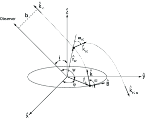
Figure 1: Schematic diagram showing the relevant angles and unit vectors defining our geometry. The unit vector $\hat{\rm k}$ denotes the photon’s direction, $\hat{\rm B}$ points in the direction of the magnetic field, and quantities with subscript “sc” correspond to the scattered photon. Other symbols are defined in the text. For illustrative purposes, two sample photon trajectories are shown: first, the unperturbed geodesic emanating from the disk; second, the modified trajectory resulting from a scattering event at ${\bf r}_{sc}$.

The observer is located at infinity with viewing angle $i$ relative to the $z$-axis in the non-rotating frame (see figure 1). The deflection angle of a photon emitted by plasma in the transiently energized inner region of the disk is $\psi$, where $\cos\psi=\cos i\cos\phi$, $\phi$ being the azimuthal angle of the emission point relative to the reference $x$-axis. These emitted photons are deflected by the black hole and intersect the observer’s detector plane at infinity. (Note that this same geometry is valid for the deflection of scattered photons as well.) The distance between the line-of-sight and the point at which the photon reaches the detector is defined as the impact parameter $b$. Using this geometry, the deflection angle of the photon’s trajectory may be obtained with the light-bending relation between $\varpi$ (the angle between the emission direction of the photon and the direction from the center of the black hole to the location of the emitter) and $\psi$, from the geodesic equation (see Beloborodov 2002)

$$\cos\psi=1-{1-\cos\varpi\over 1-R_{s}/r}\;.$$ (10)

This procedure yields the impact parameter $b=r_{e}(1-R_{s}/r_{e})^{-1}\sin\varpi$ of the photons in terms of the emitting radius $r_{e}$. A detailed description of this geometry is provided in, e.g., Luminet (1979), and a more complete accounting of POLLUX, together with several other sample applications, will appear in Falanga et al. (2011).

4 Simulations

Given the above considerations—some from prior fitting to the data (e.g., Dodds-Eden et al. 2009, Trap et al. 2011), others from earlier theoretical work (e.g., Melia 2007)—we have selected the following physical environment to model with POLLUX, the results of which are summarized in the next two subsections. We assume a radiating ring (energized by an as yet unidentified instability), $1\;R_{S}$ wide and inner radius at $3\;R_{S}$. The non-thermal particle distribution is described by the synchrotron-cooled power law in Equation (4), with an ambient azimuthal magnetic field ${\bf B}=(10\;{\rm G})\,\hat{\phi}$. The break frequency (Equation 3) is then $5.4\times 10^{15}$ Hz. Aside from the clear observational motivation for this geometry, there are also compelling theoretical reasons for expecting this type of disk instability, as discussed more extensively in Tagger & Melia (2006) and Falanga et al. (2007). Further, to examine how the polarimetric image of this instability compares with one in which scattering is important, we also assume (and report in subsection 4.2 below the impact of) a straightforward scattering halo, with uniform electron density $n_{sc}=10^{11}$ cm^-3 and radius $15\;R_{S}$, centered on the black hole. Again, for specificity, we take these particles to be thermal, with temperature $T_{sc}=10^{9}$ K.

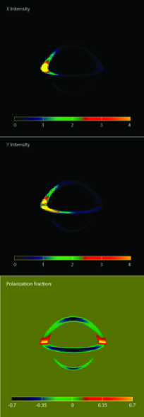
Figure 2: Polarimetric images of a radiating ring, with width $1\;R_{S}$ and inner radius $3\;R_{S}$, producing a cooled synchrotron spectrum with a break frequency at $5.4\times 10^{15}$ Hz. The images shown here correspond to the frequency range $1.6\times 10^{14}$ Hz to $2.8\times 10^{14}$ Hz, as viewed by an observer at an inclination angle of $75-80$ degrees relative to the disk’s symmetry axis. Top panel: Light polarized in the horizontal (or $x$) direction; Middle panel: Light polarized in the vertical (or $y$) direction; Lower panel: Polarization fraction defined in Equation (11).

4.1 Single Synchrotron-cooled Power Law

Figure 2 gives a sample of the results from this simulation. In all of these images, the vertical (or $y$) coordinate is parallel to the disk’s symmetry axis. The top panel shows the intensity $I_{x}$ of light polarized in the horizontal (or $x$) direction on a linear color scale. The corresponding intensity $I_{y}$ of light polarized in the $y$ direction appears in the middle panel. The bottom panel is an image (using the same spatial scale as the first two) of the polarization fraction, defined as

$$\Pi\equiv{F_{x}-F_{y}\over F_{x}+F_{y}}\;,$$ (11)

where $F_{x}$ and $F_{y}$ are the fluxes of polarized light calculated in the $x$ and $y$ directions, respectively, by integrating $I_{x}$ and $I_{y}$ over their respective solid angles, with all the usual gravitational effects—e.g., area amplification—taken into account.

The interpretation of these results is rather straightforward (see also Bromley et al. 2001). As we discuss in § 3 above, the dominant magnetic field component in this region is expected to be azimuthal. The extraordinary emissivity dominates over the ordinary, so most of the $y$-polarized light comes from the front and rear of the disk, whereas most of the $x$-polarized light comes from the sides. In addition, the disk is assumed to rotate counter-clockwise in this geometry, so the left is blue-shifted, whereas the right is red-shifted. All the general relativistic and emissivity effects together conspire to produce a shift to the left of $I_{x}$ relative to $I_{y}$. However, the polarized fraction is not affected by redshift, so the bottom image is symmetric about the vertical axis, and more clearly demonstrates the spatial dependence of the extraordinary versus ordinary emissivities. In principle, the polarization fraction varies over a broad range in values, from $-0.7$ (the negative sign meaning that $I_{y}$ is dominant over $I_{x}$) to $0.7$ (when $I_{x}$ dominates over $I_{y}$). What we see, however, is an integration of the intensity over the whole image, yielding a single polarized flux, so the net polarization fraction is never quite this high (see figure 4 below).

The polarimetric images at other energies, say $2-10$ keV, are similar to these, and will be reported as part of a more complete survey of results in Falanga et al. (2011). But we will continue our discussion of these characteristics in conjunction with figure 4 below.

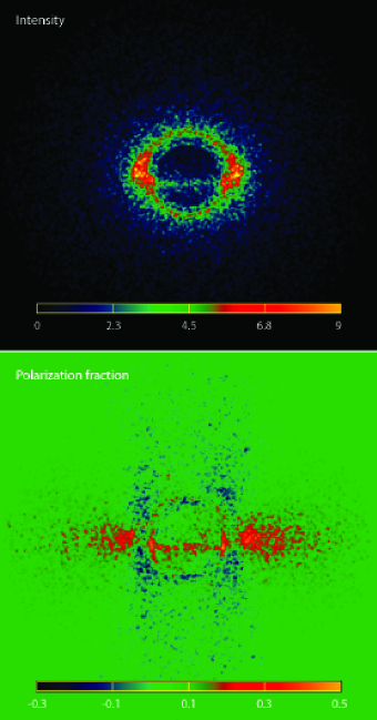
Figure 3: Same as figure 2, except here for the total intensity $I=I_{x}+I_{y}$, imaged in the frequency range $5\times 10^{17}$ Hz to $1.1\times 10^{18}$ Hz, passing through a uniform scattering halo with radius $15\;R_{S}$ centered on the black hole. Upper panel: The logarithm of total intensity; Lower panel: Polarization fraction.

4.2 Synchrotron NIR Plus Comptonized X-rays

Before doing so, however, let us examine the impact on our results of a scattering halo. Let us assume now that, in addition to the synchrotron emitting ring described above, we also have a scattering halo surrounding the black hole and inner disk region. We are not necessarily espousing the view that this is a viable model for the NIR/X-ray flare characteristics observed in recent years. If Comptonization is important in producing the X-rays, the incipient emission need not be that due to a synchrotron-cooled particle distribution. Our main goal here is to demonstrate how the images and polarization fraction (and possibly the position angle) are altered by scattering from those corresponding to the direct images.

Scattering clearly broadens the image, by a degree dependent on the density $n_{sc}$ of scattering particles. In this simulation, we have chosen a value $n_{sc}=10^{11}$ cm^-3, corresponding to a photon mean free path roughly equal to the size of the halo. Thus, virtually all of the photons emitted by the inner ring scatter at least once on their way out.

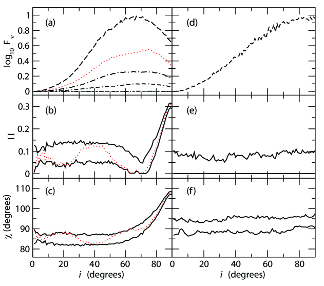
Figure 4: Panel (a): total flux density as a function of inclination angle, for various frequency ranges. From top to bottom, the 5 curves correspond to $(5\times 10^{13},9\times 10^{13})$ Hz, $(1.6\times 10^{14},2.9\times 10^{14})$ Hz, $(5\times 10^{14},9\times 10^{14})$ Hz, $(1.6\times 10^{15},2.9\times 10^{15})$ Hz, and $(5\times 10^{17},9\times 10^{17})$ Hz. Panel (b): Solid curves showing the maximum and minimum polarizations for any of the frequencies, $(2.9\times 10^{13},2.9\times 10^{19})$ Hz, included in our simulation. By way of example, the dotted curve in this panel corresponds to the polarization fraction as a function of inclination angle for the frequency range $(1.6\times 10^{14},2.9\times 10^{14})$ Hz. The rise in $\Pi$ as $i\rightarrow 40^{\circ}$ is due to the dominance of the Doppler-shifted emission from the sides of the disk, whereas the decline in $\Pi$ as $i$ increases further is due to the increasing influence of the emission from the front and rear of the disk. The position angle $\chi$ changes in concernt to reflect these varying contributions. Panel (c): The range of position angle $\chi$ (defined in Equation 12) as a function of inclination angle, for the same frequencies as in the previous two panels. Panel (d): total flux density of light scattered into the frequency range $(1\times 10^{14},2.5\times 10^{14})$ Hz. Panel (e): Same as Panel (b), except now for the scattered light (see figure 3). Here, the lower limit on $\Pi$ is zero. Panel (f): Same as Panel (c), except for the scattered light.

But scattering does more than this. It is well known that radiation passing through a scattering medium acquires a linear polarization fraction dependent on the inclination angle relative to the surface of the scattering medium (see, e.g., Conors et al. 1980). Thus, light originally polarized at the point of emission, may become more or less polarized, depending on its trajectory through to the observer. We see the tell-tale signature of this effect in the lower panel of figure 3. Notice, e.g., that portions of the image polarized in the vertical direction (in blue) now extend much farther above and below the disk. And we shall see in figure 4 below that an important consequence of scattering is a general dilution of otherwise more strongly polarized X-ray emission.

5 Key Results and Conclusions

Some of the most important results of our simulations are summarized in figure 4. With these, we can now begin to answer some of the questions posed in the introduction. First of all, a broken power-law distribution of particles emitting synchrotron radiation from an energized ring at the marginally stable orbit produces a polarization fraction at infinity of up to $\sim 15\%$ (even more for inclination angles $>70^{\circ}$) when all the relevant general relativistic effects are taken into account. Polarimetric measurements in the NIR reveal polarization fractions as high as $12\%-25\%$. The geometry we have adopted here can therefore account for these observations without the need to induce linear polarization using more complicated procedures.

Detailed fits to the observations led to the idea that the X-rays may be due primarily to the same population of electrons producing the NIR emission, though synchrotron-cooled at higher energies. The results of our simulations show that this remains a viable model even when all of the relativistic effects are taken into account. Null geodesics (and parallel transport) are not energy dependent, so the polarization properties of the X-ray component echo those of the NIR. Therefore, a prediction of this model is that both the polarization fraction and position angle $\chi$ of the X-rays should be similar to those of the infrared. Panel (c) in figure 4 shows that $\chi$, defined by the expression

$$\chi\equiv\cos^{-1}\left({F_{x}-F_{y}\over F_{x}+F_{y}}\right)\;,$$ (12)

lies somewhere between $85^{\circ}$ and $90^{\circ}$ for most inclination angles, except above $\sim 70^{\circ}$ where it can reach $\sim 110^{\circ}$ or more. These values of position angle are consistent with the fact that $F_{y}$ dominates over $F_{x}$, as one would expect when the extraordinary component is much greater than the ordinary. The increase in $\chi$ with $i$ is due to the increasing influence of redshift seen, e.g., in figure 2, which moves the core of the observed emission towards the left in these images.

Notice, however, that a different picture emerges for the X-ray characteristics when scattering is important. Panel (e) in figure 4 shows that the polarization fraction is smaller (typically smaller than $10\%$) when X-rays emerge from scattering. For many inclination angles, $\Pi$ is actually closer to $0\%$. In addition, the position angle differs from that in Panel (c), by anywhere from $\sim 5^{\circ}$ to as much as $20^{\circ}$, depending on the inclination angle.

Of course, the capability to measure $\Pi$ and $\chi$ for X-rays may be many years away, but that technology is being developed. For example, several X-ray polarimetry missions have already been studied and proposed to open up this very promising field of research over the next few years. The most advanced project today—the Gravity and Extreme Magnetism (GEM) mission (Swank et al. 2010), is planned for launch in 2014, with the primary goal of studying the polarimetric properties of the soft X-ray emission from bright black holes and neutron stars. Unfortunately, the GEM instruments will not be sensitive enough to study a relatively weak source, such as Sgr A*. Indeed, for fluxes less than 1 milliCrab (the intensity reached by Sgr A* at the peak of the brightest flares), GEM would need a net observing time of more than 100 ks to detect a polarization fraction of 10% or lower. But Sgr A*’s flares never last longer than 3 hr, so it would not be feasible to obtain such a deep exposure. Moreover GEM, and even other future polarimetry projects, such as POLARIX (Costa et al. 2010), could not provide angular resolutions better than $\sim 1^{\prime}$, making it very difficult to identify the origin of a polarized signal from a crowded region, such as we have at the galactic center. Nonetheless, this field is only in its infancy. More promising missions, with better sensitivity and spatial resolution, will no doubt follow in the years to come. And our results demonstrate the power of future simultaneous polarimetric observations in both the NIR and X-ray portions of the spectrum.

References

- Baganoff (01) Baganoff, F. K. et al. 2001, Nature, 413, 45
- Baganoff (03) Baganoff, F. K. et al. 2003, ApJ, 591, 891
- Balick (74) Balick, B. and Brown, B. L. 1974, ApJ, 194, 265
- Belanger (04) Bélanger, G. et al. 2004, ApJ Letters, 601, L163
- Belanger (05) Bélanger, G. et al. 2005, ApJ, 635, 1095
- Belanger (06) Bélanger, G. et al. 2006, ApJ, 636, 275
- Beloborodov (02) Beloborodov, A. M. 2002, ApJ Letters, 566, L85
- Broderick (05) Broderick, A. E. & Loeb, A. 2005, MNRAS, 363, 353
- Bromley (01) Bromley, B. C., Melia, F. & Liu, S. 2001, ApJ Letters, 555, L83
- Connors (77) Connors, P. A. & Stark, R. F. 1977, Nature, 269, 128
- Connors (80) Connors, P. A., Piran, T. V., & Stark, R. F. 1980, ApJ, 235, 224
- Costa (10) Costa, E. et al. 2010, Exp. Astron., 28, 137
- Crocker (10) Crocker, R. et al. 2010, Nature, 463, 65
- Davis (09) Davis, S. W. et al. 2009, ApJ, 703, 569
- Dexter (09) Dexter, J., Agol, E., and Fragile, P. C. 2009, ApJ Letters, 703, 142
- Dodds (09) Dodds-Eden, K. et al. 2009, ApJ, 698, 676
- Doeleman (08) Doeleman, S. S. et al. 2008, Nature, 455, 78
- Dolence (09) Dolence, J. C. et al. 2009, ApJS, 184, 387
- Dovciak (04) Dovciak, M. et al. 2004, MNRAS, 350, 745
- Eckart (04) Eckart, A. et al. 2004, AA, 427, 1
- Eckart (06) Eckart, A., Schödel, R., Meyer, L., Trippe, S., Ott, T., & Genzel, R. 2006, AA, 455, 1
- Falanga (07) Falanga, M., Melia, F., Tagger, M., Goldwurm, A., & Bélanger, G. 2007, ApJ Letters, 662, L15
- Falanga (11) Falanga, M., Melia, F., & Goldwurm, A. 2011, ApJ, in preparation
- Falcke (97) Falcke, H. & Melia, F. 1997, ApJ, 479, 740
- Falcke (00) Falcke, H., Melia, F. & Agol, E. 2000, ApJ Letters, 528, L13
- Genzel (03) Genzel, R. et al. 2003, Nature, 425, 934
- Ghez (03) Ghez, A. et al. 2003, ApJ Letters, 586, L127
- Goldwurm (03) Goldwurm, A.et al. 2003, ApJ, 584, 751
- Hawley (96) Hawley, J. F., Gammie, C. F. & Balbus, S. A. 1996, ApJ, 464, 690
- Hollywood (97) Hollywood, J. M. & Melia, F. 1997, ApJ Supp, 112, 423
- Hornstein (07) Hornstein, D. et al. 2007, ApJ, 667, 900
- Kunneriath (10) Kunneriath, D. et al. 2009, AA, 517, A46
- Liu (01) Liu, S. & Melia, F. 2001, ApJ Letters, 561, L77
- Liu (02) Liu, S. & Melia, F. 2002, ApJ Letters, 573, L23
- Liu (04) Liu, S., Petrosian, V., & Melia, F. 2004, ApJ Letters, 611, L101
- Liu (06) Liu, S., Melia, F., Petrosian, V., & Fatuzzo, M. 2006, ApJ, 647, 1099
- Luminet (79) Luminet, J.-P. 1979, AA, 75, 228
- Markoff (01) Markoff, S., Falcke, H., Yuan, F., & Biermann, P. L. 2001, AA Letters, 379, L13
- Marrone (08) Marrone, D. P. et al. 2008, ApJ, 682, 373
- Melia (92) Melia, F., 2002, ApJ Letters, 397, L25
- Melia (07) Melia, F. 2007, The Galactic Supermassive Black Hole (New York: Princeton University Press)
- (42) Melia, F., Bromley, B. C., Liu, S., & Walker, C. K. 2001a, ApJ Letters, 554, L37
- (43) Melia, F., Liu, S. & Coker, R. F. 2000b, ApJ Letters, 545, L117
- Melia (02) Melia, F. et al. 2002, ApJ Letters, 554, L37
- Misra (93) Misra, R. & Melia, F. 1993, ApJ Letters, 419, L25
- Nayakshin (98) Nayakshin, S. & Melia, F., 1998, ApJ Supp, 114, 269
- Nishiyama (09) Nishiyama, S. et al. 2009, ApJ Letters, 702, L56
- Noble (07) Noble, S. C. et al. 2007, CQG, 24, 259
- Pacholczyk (70) Pacholczyk, A. 1970, Radio Astrophysics. Nonthermal Processes in Galactic and Extragalactic Sources (San Franciso: Freeman)
- Porquet (03) Porquet, D. et al. 2003, AA Letters, 407, L17
- Porquet (08) Porquet, D. et al. 2008, AA, 488, 549
- Rockefeller (04) Rockefeller, G., Fryer, C. L., Melia, F., & Warren, M. S. 2004, ApJ, 604, 662
- Ruffert (94) Ruffert, M. & Melia, F. 1994, AA Letters, 288, L29
- Rybicki (85) Rybicki, G. B. & Lightman, A. P. 1985, Radiative Processes in Astrophysics (New York: Wiley)
- Schnittman (10) Schnittman, J. D. & Krolik, J. H. 2010, ApJ, 712, 908
- Schodel (02) Schödel, R. et al. 2002, Nature, 419, 694
- Shcherbakov (11) Shcherbakov, R. V. & Huang, L. 2011, MNRAS, 410, 1052
- Swank (10) Swank, J., et al. 2010, in “X-ray Polarimetry: A New Window in Astrophysics,” eds. Ronaldo Bellazzini, Enrico Costa, Giorgio Matt and Gianpiero Tagliaferri. Cambridge University Press, p. 251
- Tagger (06) Tagger, M. & Melia, F. 2006, ApJ Letters, 636, L33
- Trap (11) Trap, G. et al. 2011, AA, 528, 140
- Yuan (04) Yuan, F., Quataert, E., & Narayan, R. 2004, ApJ, 606, 894
- Zamaninasab (11) Zamaninasab, M. et al. 2011, MNRAS, 413, 322
- Zhao (04) Zhao, J.-H., Hernstein, R. M., Bower, G. C., Goss, W. M., & Liu, S. M. 2004, ApJ Letters, 603, L85
- Yusef (00) Yusef-Zadeh, F., Melia, F., & Wardle, M. 2000, Science, 287, 85
- Yusef (06) Yusef-Zadeh, F. et al. 2006, ApJ, 644, 198
- Yusef (09) Yusef-Zadeh, F. et al. 2009, ApJ, 706, 348