Response of the Shockley surface state to an external electrical field:
A density-functional theory study of Cu(111)

Abstract

The response of the Cu(111) Shockley surface state to an external electrical field is characterized by combining a density-functional theory calculation for a slab geometry with an analysis of the Kohn-Sham wavefunctions. Our analysis is facilitated by a decoupling of the Kohn-Sham states via a rotation in Hilbert space. We find that the surface state displays isotropic dispersion, quadratic until the Fermi wave vector but with a significant quartic contribution beyond. We calculate the shift in energetic position and effective mass of the surface state for an electrical field perpendicular to the Cu(111) surface; the response is linear over a broad range of field strengths. We find that charge transfer occurs beyond the outermost copper atoms and that accumulation of electrons is responsible for a quarter of the screening of the electrical field. This allows us to provide well-converged determinations of the field-induced changes in the surface state for a moderate number of layers in the slab geometry.

I Introduction

Surface statesShockley (1939); bk: (a, b); Han are long known to significantly affect the properties of surfaces in a host of ways. This is particularly so when the surface state crosses the Fermi level, rendering it metallic. Such states provide the possibility of low-energy adsorption and enhancement of transport. On the close-packed (111) surfaces of noble metals, such states have their minima at the center of the surface Brillouin zone ($\bar{\Gamma}$) in the bulk $L$ gap, have minimal angular anisotropy, and are well approximated by free-electron dispersion.Gartland and Slagsvold (1975); Reinert et al. (2001) Since the energy difference between the Fermi level and the bottom of the band is small, so is the Fermi wave vector, leading to a Fermi wavelength that is nearly an order of magnitude larger than that of typical bulk Fermi wavelengths. Furthermore, confinement to the surface leads only to slow decay in directions perpendicular to the surface plane, Fig. 1. Arguably the most dramatic outcome is the observation of quantum corrals and mirages on surfaces. Crommie et al. (1993); Heller et al. (1994); Crommie et al. (1995); Fiete and Heller (2003) These states can also produce ordered superstructures of adsorbed species.Hyldgaard and Persson (2000); Repp et al. (2000); Hyldgaard and Einstein (2002); bk: (c); Hyldgaard and Einstein (2003); Stepanyuk et al. (2003); Hyldgaard and Einstein (2005); Nanayakkara et al. (2007)

A question of both fundamental and practical concern is the sensitivity of these metallic surface states to perturbations. Moderately strong perturbations such as chemisorption can easily destroy the surface state,Chen and Smith (1989); Dudde et al. (1990) or create overlayer resonances.Schiller et al. (2008); Fischer et al. (1994); Breitholtz et al. (2007) There is also a theoretical prediction that alkali-overlayer formation can lead to a localization (for dynamics parallel to the surface) of high-energy electrons in a resonance state.Chis et al. (2007) On the other hand, weak perturbations can allow the state to survive but with an altered dispersion relation (typically a shifted minimum and a changed curvature).Carlsson et al. (1997); Schiller et al. (2008) This offers the exciting possibility to manipulate the Fermi wavelength and effective mass of the state, if one can understand in detail how perturbations such as adsorption affect dispersion.

Figure 1: (Color online) Contours of the $\bar{\Gamma}$-point surface-state density. Yellow (red, blue) surfaces correspond to high (medium, low) density. The density is largest outside the surface, and lowest in the planes formed by the atoms. Graphics generated with VESTA.Momma and Izumi (2008)

However, adsorption typically leads to several different changes to the surface.Lindell et al. (2005) First, there can be charge transfer, producing an electric field due to the resulting surface dipole. (There could also be effects from the intrinsic dipole of an organic adsorbate.) Second, there can be correlated electron hopping such as characteristic of covalent bonds. Third, the adsorbate will perturb the tails into the vacuum of the metal-surface electron density. Lindell et al. (2005) Furthermore, as dipole-producing adsorbates approach each other, they create a depolarizing field that decreases the dipole, consistent with experiments for Na atoms on Cu(001).Fratesi et al. (2010) Hence, the prospect of predicting how a particular adsorbate modifies the surface state poses a considerable challenge.

In this paper, we instead focus on just the first aspect of the adsorption bond, that due to charge transfer. Specifically, we look at the effect that a uniform electric field normal to the surface has on the surface state. This problem also has advantages over a direct study of a pure ionic bond: the electric field is uniform, and the screening is well confined to the direction perpendicular to the substrate. Furthermore, this simple scenario bears on the more complicated geometry involved with the effect of strong fields between STM tips and substrates.Limot et al. (2003); Kröger et al. (2004)

For over four decades,Lang and Kohn (1970) with increasing sophistication, theoreticians have used density-functional theory (DFT) in various implementationsLang and Kohn (1970); Weber and Liebsch (1987); Chizmeshya and Zaremba (1988); Kiejna (1995); Hult et al. (1996); Feibelman (2001); Inglesfield (1991); Negulyaev et al. (2011); Achilli et al. (2007) to examine the effect of static perpendicular electric fields on the electronic properties of simple metal surfaces (until relatively recently, typically jellium-like). Trying to understand experiments related to self-diffusion on Pt(001), Feibelman discussed how such electric fields can be used to tune diffusion barriers and possibly alter the dominant mechanism of mass transport.Feibelman (2001) Negulyaev et al. showed that such fields could serve as a switching tool for magnetic states in atomic-scale nanostructures.Negulyaev et al. (2011) However, we know of no DFT study of the effect perpendicular electric fields on metallic surface states.

We further note that understanding the surface response to a perpendicular electric field and the formation of an image plane are fundamental building blocks in the study of the van der Waals interactions.Lif ; Zaremba and Kohn (1976); Apell (1981); Persson and Apell (1983); Persson and Zaremba (1984); Liebsch (1987); Rydberg et al. (2000) The image plane is available from DFT calculationsHult et al. (1996); Andersson et al. (1998); Hult et al. (1999, 2001) and the handling of screening is a central element in the vdW-DF method.Dion et al. (2004); Thonhauser et al. (2007); Lee et al. (2010) Knowledge of the image plane position permits an approximation of multipole effects,Zaremba and Kohn (1976); Rydberg et al. (2003) and hence a quantitative study of interactions of, for example, atoms and molecules at noble-metal surfaces.Zaremba and Kohn (1977); Nordlander and Harris (1984); Andersson and Persson (1993); Lee et al. (2011) The image plane is also important for ensuring transferability over a range of different binding distances, for example, in molecular crystals.Kleis et al. (2008); Berland and Hyldgaard (2010); Berland et al. (2011)

Much of our exploration was motivated by a desire to manipulate the surface states that mediate the interactions between anthraquinone (AQ) molecules on Cu(111):Pawin et al. (2006) the giant regular honeycomb formed spontaneously by them are likely related to such interactions.Kim and Einstein (2011) Alternatively, the pores in the honeycomb can be viewed as an array of two-dimensional (2D) quantum dots. The stabization of the pattern may be due to the population—from the metallic surface state—of the 2D orbitals of the dots, forming what amounts to closed-shell, 2D-noble-gas-like quasiatoms.Wyrick et al. (2011) By manipulating the surface state, we hope to tune its Fermi wave vector (and, concomitantly, its effective mass) and thereby enhance or destabilize different superlattice structures. A major goal of this study of surface-state response is to gain the ability to engineer novel structures on surfaces. Furthermore, the standing waves within the honeycomb cells, arising from these surface states, are believed to determine the potentials that small molecules like CO encounter when adsorbing within the cells. Cheng et al. (2010) These cells form a set of identical nanostructures with thermodynamic-like behavior that differs significantly from that found when these molecules adsorb on large defect-free flat surfaces.

Most traditional DFT implementations rely on supercells to model surfaces, with slabs separated by vacuum. However, since pairs of Shockley surface states on opposite sides of a slab hybridize, the energy and dispersion are affected, with ensuing loss of accuracy. Use of very thick slabs can marginalize the hybridization effects, but such a brute-force approach is computationally expensive and more susceptible to numerical noise. In this paper, we present a method which extracts proper, un-hybridized, surface states from standard supercell-DFT studies for geometries with moderate slab thicknesses. Our method is based on a simple rotation in the Hilbert space spanned by the two Kohn-Sham (KS) metallic surface states that are found in underlying semilocal DFT calculations. We use our method to characterize the response of the Cu(111) surface state, but it should also be useful for the study of other, more complex, material systems.

The KS-rotation method presented here is complementary to the use of more advanced DFT implementations, such as the embedding Green function method,Inglesfield (1981); Nekovee and Inglesfield (1992); Szunyogh et al. (1994, 1995); Ishida (2001); Lazarovits et al. (2002); Butti et al. (2005) which effectively model a semi-infinite surface. The embedding method can also handle an external field.Achilli et al. (2007) As our study is based on a traditional DFT implementation, we do not correctly describe the image-potential behavior, for which GW calculationsEguiluz et al. (1992); Sau et al. (2008) are normally required. The embedded method allows an explicit inclusionNekovee and Inglesfield (1992); Szunyogh et al. (1994, 1995); Butti et al. (2005) of an image-like behavior and can therefore determine image-potential states in DFT. The inclusion of this image-like behavior would likely also improve the accuracy of the evanescent part of the surface states found in the slab analysis. In spite of these benefits of an embedding method, we believe it is also important to continue to seek simple mechanisms to enhance the accuracy in widely used (for examples, Refs. Kokalj and Causà, 1999; Carlsson and Hellsing, 2000; Fichthorn and Scheffler, 2000; Bogicevic et al., 2000; Fölsch et al., 2004; Chis and Hellsing, 2004; Luo and Fichthorn, 2005; Da Silva et al., 2006; Yu et al., 2006; Breitholtz et al., 2007; Forster et al., 2007; Wong et al., 2007; Howe et al., 2010; Hayat et al., 2010; Bjork et al., 2010; Dyer and Persson, 2010) slab-geometry DFT studies of surface states.

The plan of this paper is as follows. In Sect. II we discuss our computational methods, paying particular attention to a simple yet unambiguous and robust way to accurately decouple the surface states on the two sides of the slab and to obtaining a faster convergence as a function of slab thickness. In Sect. III we characterize the surface state with no electric field, while in Sect. IV we describe the changes in the wavefunctions, potential profile, and dispersion in the presence of an applied perpendicular field. Sect. V discusses the screening of this electric field, deriving the relative contribution of the electrons in the surface state. It also makes comparisons with experimental data and illustrates the decoupling method for benzene on Cu(111). Finally, Sect. VI offers conclusions about the impact of these changes in the surface state.

II Computational methods

The electronic structure is obtained with DFT within the generalized-gradient approximation (GGA) for exchange-correlation using the PBE Perdew et al. (1996) version. For these calculations, we use the ultrasoft pseudopotential plane-wave code ACAPO , \cite{ACAPO with an energy cutoff of 400 eV,Com (a) and a k-sampling of 16$\times$16$\times$1. The KS states required to obtain the surface-state dispersion is calculated non-self consistently in a post-processing Harris functional calculation Harris (1985) in which the wave vectors were sampled with a grid spacing of 0.01 $K$, where $K$ is the size of the shortest in-plane reciprocal-lattice vector. The Cu(111) surface is modeled as a finite slab in a supercell since the plane-wave scheme restricts us to using periodic boundary conditions. The top and bottom copper layers in two adjacent supercells are separated by $12{\rm\AA}$, thus insuring negligible cross-coupling. The lattice constant of the slab is set to that of copper, $a=3.65{\rm\AA}$, as obtained in a separate bulk PBE calculation. The electrical fields used in this study only slightly perturb the electronic structure of the surface, and we find no significant relaxations of the atoms of the surface slab; the atoms are therefore frozen in their truncated bulk positions.Com (b) A dipole layer in the vacuum region induces an external electrical field normal to the copper slab.Bengtsson (1999); Neugebauer and Scheffler (1992) Both positive and negative electrical fields are studied in a single calculation.

II.1 Issues with coupled surface states

The finite slab geometry makes the surface state couple to both the two sides of the slab, and therefore challenges the analysis of surface state response to an external perturbations. In the upper panel of Fig. 2, the full curves show the sum-projected density of the KS wavefunctions with surface-state character, $\psi^{\rm KS}_{i}(\mathbf{k})$ at the $\bar{\Gamma}$ point,

$$\rho^{\rm KS}_{i}(z)=\int\mathrm{d}x\,\int\mathrm{d}y\,|\psi^{\rm KS}_{i}(x,y,z)|^{2},$$ (1)

for a six-layer thick copper slab in zero external field. These states couple equally to both sides of the slab, rather than being localized on one side. They therefore lack the characteristic exponential decay into the bulk. In a hybridization, or tight-binding picture, these KS states can be viewed as linear combinations of surface-localized (SL) states that hybridize in a finite slab geometry. For zero electrical field, the KS states form symmetric and anti-symmetric combinations of the underlying SL states (which provide an accurate description of the actual surface-state behavior). The dashed lines in the top panel of Fig. 2 shows the sum-projected densities, $\rho_{i}^{\rm SL}$, of these SL states. The SL states exhibit “good” surface-state properties, like exponential decay into the bulk and localization at the surface. For sufficiently large slabs, these SL states are good representations of the proper surface states, i.e., surface states as they would have been calculated in an accurate DFT of a semi-infinite bulk system.

Figure 2: (Color online) Issues with surface-state hybridization that arise because of the finite slab geometry. The upper panel shows the sum-projected surface-state densities obtained for a six layer wide copper slab. The full lines shows the Kohn-Sham (KS) states with surface-state character. The dashed lines show the surface-localized (SL) states for which we here present a simple but robust determination (since the SL states provide a more accurate description of genuine surface-state behavior). The lower panel shows the electric field variation of the surface state for a 15-layer slab calculation using the plane-wave code DACAPO. The full line shows the least-squares fit to decoupled surface-state energies as obtained for the SL states, Sec. IV.B.

In the lower panel of Fig. 2 the filled (red) circles show, for different external fields, the KS eigenvalues for the states with surface-state character, $\epsilon_{i}^{\rm KS}$. These results were obtained for a 15 layer thick slab. The jump at $E=0$ in the KS calculation of the minimum surface-state energy, $\epsilon^{\rm KS}(0)$, indicates an avoided crossing, which further supports the picture of a coupled two-level system. Since the field influences both the properties of the underlying states and the linear combination making up the KS states, it is a challenge to deduce the inherent response of the proper surface states.

II.2 Decoupling of surface states

This subsection presents our numerically robust method to construct the (pair of) SL states from the KS surface states of the slab. The full line in the bottom panel of Fig. 2 shows the effective Fermi level shifts for the SL result. The continuity of this result contrasts the singular response which appears in an analysis based directly on the KS states (shown as [red] dots). Our assumption is that the KS surface states arise exclusively from hybridization of the actual SL states; we assume that these do not couple to bulk states or surface resonances. In this case, we can for a given $\mathbf{k}$ set up a bonding/antibonding Hamiltonian for this SL two-level system:

$$\cal{H}(\mathbf{k})=\left(\begin{array}[]{cc}\epsilon(\mathbf{k})+W(\mathbf{k})&\Omega(\mathbf{k})\\ \Omega^{*}(\mathbf{k})&\epsilon(\mathbf{k})-W(\mathbf{k})\end{array}\right)$$ (2)

Here $\epsilon(\mathbf{k})\pm W(\mathbf{k})$ gives the energy of the uncoupled states, where $W$ is the detuning between the levels and $\Omega$ is the coupling. In terms of them, the eigenvalues of the KS wavefunctions are given by

$$\epsilon^{\rm KS}_{1,2}=\epsilon\pm\sqrt{W^{2}+|\Omega|^{2}}\,,$$ (3)

which follows from the invariance of $\mathrm{Tr}\,\cal{H}$ and $\mathrm{Det}\,\cal{H}$. As the slab size increases, $\Omega\rightarrow 0$ and the eigenvalues of the decoupled surface states reduce to $\epsilon\pm W$. The key observation is that the SL state energy $\epsilon$ converge much faster as the slab size increases than the coupling parameter $\Omega$ vanishes. The same is generally true of the detuning parameter $W$; even at $E=0$ (when the correct detuning must vanish identically), we find (below) that the numerical value of $W$ converges fairly well before the accumulation of numerical noise eventually destroys this behavior. Therefore, by constructing $\cal{H}$ of Eq. (2), we can characterize the surface-state properties to high accuracy, with a smaller unit cell than what is required for the KS to decouple due to asymmetry induced by small-scale numerical effects. In general a SU(2) rotation is needed to construct the SL basis states and $\cal{H}$ as we seek a linear combination of the KS wave-functions $\psi_{i}(\mathbf{k})$ that localizes the state on one side of the slab through constructive and destructive interference. However, when we can identify the symmetry point of the unit cell in the xy-plane, we can ensure that both KS states have the same variation in the complex plane. This is done, for example, in the present Cu(111) slab study, by setting the KS states real at this symmetry point via multiplication by a simple phase factor: $\psi_{i}\rightarrow\exp(\mathrm{i}\eta)\psi_{i}$. The transformed KS states must then have the same complex-phase variation across the unit cell because the KS states are Bloch functions: they can be written as $\psi_{i}(\mathbf{r})=u_{i}(\mathbf{r})e^{\mathrm{i}\mathbf{k}\mathbf{r}}$, where $u_{i}(\mathbf{r})$ has the same periodicity as the supercell and can be chosen real.Kohn (1959) With this transformation, the full SU(2) transformation reduces to an O(2) rotation $R$ in the Hilbert space:

$$\left(\begin{array}[]{c}\phi_{1}\\ \phi_{2}\end{array}\right)=\left(\begin{array}[]{cc}\cos\theta&-\sin\theta\\ \sin\theta&\cos\theta\end{array}\right)\left(\begin{array}[]{c}\psi_{1}\\ \psi_{2}\end{array}\right)\,.$$ (4)

To determine the value of $\theta$, we choose a condition of maximal localization (MaxLoc), that is, we minimize the sum of the variances of the generated wavefunctions

$$F(\theta)=\sum_{i}|\langle\phi_{i}|z_{i}^{2}|\phi_{i}\rangle|-|\langle\phi_{i}|z_{i}|\phi_{i}\rangle|^{2}\,.$$ (5)

Such a condition has also been used to construct the generalized-Wannier functions. Marzari and Vanderbilt (1997) The matrix transformation that corresponds to this rotation is $H\rightarrow RHR^{\rm T}=H_{\rm SL}$. Thus,

$$\left(\begin{array}[]{cc}\epsilon_{1}^{\rm KS}&0\\ 0&\epsilon_{2}^{\rm KS}\end{array}\right)\rightarrow\left(\begin{array}[]{cc}\bar{\epsilon}^{\rm KS}+\frac{1}{2}\Delta\epsilon^{\rm KS}\cos 2\theta&\frac{1}{2}\Delta\epsilon^{\rm KS}\sin 2\theta\\ \frac{1}{2}\Delta\epsilon^{\rm KS}\sin 2\theta&\bar{\epsilon}^{\rm KS}-\frac{1}{2}\Delta\epsilon^{\rm KS}\cos 2\theta\end{array}\right)\,.$$ (6)

Here $\bar{\epsilon}^{\rm KS}=(\epsilon_{1}^{\rm KS}+\epsilon_{2}^{\rm KS})/2$ and $\Delta\epsilon^{\rm KS}=(\epsilon_{1}^{\rm KS}-\epsilon_{2}^{\rm KS})/2$ By comparing to Eq. (3), we identify the SL-hybridization parameters, $\epsilon=\bar{\epsilon}^{\rm KS}$, $W=(\Delta\epsilon_{\rm KS}/2)\cos(2\theta)$, and $\Omega=(\Delta\epsilon_{\rm KS}/2)\sin(2\theta)$. We note that $\Omega$ is real because we can here work with an O(2) rotation. For perfectly symmetric surfaces we have $\theta=\pi/4$, and the surface-state energy is then the average of the eigenvalues of the two states. Thus, the full machinery discussed here is not required. For certain perturbations, like adsorbate systems, a less elegant solution is to use symmetric adsorbates on both sides of the slab. Such a brute-force approach has the drawbacks of increased computational costs and fewer layers with a bulk-like behavior; furthermore, wave functions are not decoupled. Strong asymmetric perturbations, such as halogen overlayers, lead to $W\gg\Omega$ and a natural decoupling of the states. However, a natural decoupling does not happen for weak perturbations, like adsorbates bound by van der Waals interactions,Berland et al. (2009) or for dilute chemisorbed overlayers, where $\Omega\sim W$ unless a huge number of layers are used, typically beyond the computational feasibility.

II.3 Convergence of surface-state properties

Our method to construct the SL states significantly reduces the number of layers needed to accurately characterize the surface state; however, the slab still must be thick enough to describe most of the relatively slow decay into the bulk. We also confirm that the MaxLoc condition (see Eq. 5) properly decouples the two states by comparing with the results for a 24 layer calculation, where decoupling arises numerically as $\Omega\rightarrow 0$.

Table 1: Convergence of the surface state with slab thickness. All three columns of energies are in meV. The bold numbers, for 15 layers, are used for the rest of this paper.

# layers	$\epsilon_{F}-\epsilon(0)$	$\Omega^{(E=0)}$	$W^{(E=0)}$
6	520	272	$0.24$
9	464	113	$0.38$
12	449	50	$0.17$
15	443	23	${\bf 0.81}$
18	443	10	$1.34$
24	442	2	$11.0$

Table 1 shows the calculated SL state parameters for for different slab thicknesses at zero electrical field. The Fermi energy $\epsilon_{\rm F}$ relative to $\epsilon(0)$ converges to the sub-meV level for a 15-layer slab if the decoupling method is used. For a six-layer slab the surface-state energy differs from the converged value by 80 meV, or about 20%; we consider it a minimum slab thickness for an approximate account of the surface state, which can be useful for studying surface-state shifts for adsorbates-systems requiring a large supercell in the in-plane direction. We find that coupling $\Omega$ decays significantly slower than the value of $\epsilon_{F}-\epsilon(0)$ converges, a fact which as mentioned above motivates our approach. We note that the value of 272 meV for six layers will almost deplete one of the two surface-related KS bands (while driving the other at least partially into the energy range of bulk states). Nevertheless, the corresponding result for the effective depth of the surface-state, Fermi see, $\epsilon_{F}-\epsilon(0)$ differs from the converged value by merely 57 meV. For 15 layers $\Omega$ reduces to 23 meV, while the $\epsilon_{F}-\epsilon(0)$ is converged to within less than an meV.

II.4 Effects of numerical noise on optimal slab geometry

The nonzero value of the detuning $W$ at zero electrical field stems purely from numerical noise and grid effects, since the slab geometry is symmetric. The upper panel of Fig. 4 shows the KS states for different electrical fields. For zero electrical field, the slight asymmetry of the curves hints of the nonzero $W$. For larger fields, the KS states clearly favor one side of the slab, but even for $E=0.36{\rm V/\AA}$, the wavefunctions are localized on both sides of the slab. The inserts illustrate (purple dot) the coordinate in the 2D space $(W,\Omega)$, with magnitude $(\epsilon^{\rm KS}_{1}-\epsilon^{\rm KS}_{2})/2$, constructed using the MaxLoc condition. The detuning grows as the electrical field increases, while the coupling remains roughly constant. For six layers the two KS surface-state densities are fully symmetric as shown in the upper panel of Fig. 2. For even wider slabs, the coupling reduces, and the surface-state densities becomes increasingly asymmetric; for 24 layers, we find that the surface states localize almost exclusively on one side of the slab, consistent with a detuning five times larger than the coupling $\Omega$. That $\epsilon^{\rm KS}\approx\epsilon$ for 24 layers reflects this finding and the general expectation that increasing the number of layers must eventually decouple the KS and ensure an automatic approach to the more meaningful SL states. Nevertheless, we find that the increasing value of $W$ for slabs with than 15 layers is the sole reason for this decoupling. As this increase in $W$ (for $E=0$) is solely an expression of an accumulation of numerical noise (with the number of atoms and electrons), we conclude that such brute-force decoupling is not desirable. We propose instead to use the maximum-localization approach to identify the genuine surface-state behavior and avoid such numerical noise. In this study we use 15 layers, as it is an optimum between a converged value of $\epsilon$ and a minimal numerical noise; our approach converges the surface-state energies to meV accuracy.

III Surface state dispersion in zero electrical field

Our calculations of the surface-state dispersion in zero electrical field are presented in this section and compared to experimentalJeandupeux et al. (1999); Kevan and Gaylord (1987) and earlier theoretical studies. Hyldgaard and Einstein (2003); Courths et al. (2001) We find that the surface state is practically isotropic even for $k\equiv|\mathbf{k}|>2.5k_{F}$, and that non-parabolicity becomes significant once $k$ exceeds $k_{F}$. Figure 3 shows the surface-state dispersion as a function of the absolute value of $\mathbf{k}$. The filled (green) circles indicate the calculated values of $\epsilon(\mathbf{k})-\epsilon_{F}$, which have been sampled evenly on a $k_{x},k_{y}$-grid, while the (red) crosses indicate the energies obtained for $k_{y}=0$. That they align to form a curve shows that the surface state is isotropic, even as far as $\sim 2.5|\mathbf{k}_{F}|$. This isotropy is further evidenced by the circular constant-energy contours displayed in the insert. The full curve gives the parabolic dispersion, while the dashed includes non-parabolicity via a quartic term:

$$\epsilon(k)-\epsilon(0)=\frac{\hbar^{2}k^{2}}{2m}-\alpha k^{4}+\mathcal{O}(\mathbf{k}^{6})\,,$$ (7)

with parameters obtained as described in the following paragraph. These curves show that up to about the $k_{F}$, the dispersion is well described by a parabolic form, but for larger wave vectors, non-parabolicity is significant. The deviation from a parabolic-dispersion behavior has been observed experimentally and can be understood in terms of an $s$-band tight-binding model.Bürgi et al. (2000) We expand $\epsilon({\mathbf{k}})$ as given by the standard Hamiltonian and find:

$$\epsilon({\mathbf{k}})-\epsilon(0)\propto 1-\frac{1}{3}\cos(k_{x}a)-\frac{2}{3}\cos\left(\frac{k_{x}a}{2}\right)\cos\left(\frac{\sqrt{3}k_{y}a}{2}\right)$$

$$=\frac{1}{4}(ka)^{2}-\frac{1}{64}(ka)^{4}+\frac{10+\cos(6\theta)}{23040}(ka)^{6}+\mathcal{O}(k^{8})\,.$$ (8)

where $\theta\equiv\arctan(k_{y}/k_{x})$ and $a=2.58{\rm\AA}$ is the nearest-neighbor distance. Thus, the quartic correction is negative (albeit much smaller than found in the DFT calculation), and anisotropy does not appear until the $k^{6}$ term.sub Table 2 gives deduced surface-state properties and compares them to other studies. In obtaining these values, we only needed data points obtained for $k_{y}=0$, since we have amply demonstrated the isotropic surface-state dispersion; this procedure also avoids excessive weighting of large-$|\mathbf{k}|$ values, as the number of 2D grid points grows approximately linearly with the wave-vector magnitude. Our values for the effective Fermi level is similar to earlier experimental and calculated values. Our value is somewhat smaller than that given in Ref Butti et al., 2005, which is based on a semi-infinite approach including an image potential. Our value for the effective mass is smaller than those of the earlier studies, which is partly a result of the fitting procedure used to obtain its value. A parabolic fit is often used to extract the effective mass from the dispersion curve; however, the effective mass is defined by the second-order Taylor expansion of the dispersion curve, not by an optimal parabolic fit to a curve that may deviate from parabolicity. To properly extract the terms in the Taylor expansion with a polynomial fit, we rely only on values fairly close to the $\bar{\Gamma}$ point and, in addition, include higher-order terms in the fit to minimize their influence on the extraction of the lower-order ones. It is possible to avoid the influence of quartic terms on the effective mass with a purely parabolic fit, but this requires that we restrict the domain to data points very close to the $\bar{\Gamma}$ point. This has the disadvantage that the influence of noise is larger. In detail, our approach is as follows: first, the effective mass $m$ is obtained with least-squares using a fourth-order polynomial fit for the six smallest $\mathbf{k}$ points (corresponding to 6% of the reciprocal vector); next, we keep the mass fixed and determine $\alpha$ using a sixth-order polynomial using all 20 data points. The correspondence with the data points of Fig. 3 for small and medium $|{\mathbf{k}}|$ corroborates our procedure, as just described. If we instead include ten data points and fit to a purely parabolic dispersion, we find a mass of 0.38$m_{e}$, closer to that of earlier studies (listed in Table 2). Thus, that our deduced mass is smaller than previously obtained values relates to our use only of data points close to the $\bar{\Gamma}$ point and our inclusion of higher-order polynomial terms. The quartic prefactor $\alpha$ compensates somewhat for the smaller mass, and the Fermi wavelength $\lambda_{F}$ and wave vector $k_{F}$ are in good agreement with earlier results. That sensitivity to fitting domain (parabolic fitting) was discussed in Ref Butti et al., 2005. They note that when comparing with experimental data, it is important that same procedure is used in both cases. We argue that, ideally, all parameters should be defined in terms of the Taylor expansion. When they use a minimal sampling of $\mathbf{k}$ points around the $\bar{\Gamma}$ point, they obtain an effective mass of $0.303m_{e}$, which is closer to, and even smaller than the mass we obtain. The importance of making sure that higher-order terms do influence the extraction of the effective mass is also reflected in the significant non-parabolic dispersion that Becker et al.Becker et al. (2006) found for Ag(111). They extracted the effective mass by considering only data point collected close to the $\bar{\Gamma}$ point.

Table 2: Properties of the surface state. The value $\epsilon_{F}-\epsilon(0)$ is the difference between the Fermi surface and the minimum of the surface state $\epsilon(0)$. Also listed are comparisons of our values of the effective mass, surface-state Fermi wavelength and wavevectors, $m,\lambda_{F},k_{F}$. Our DFT value for the quartic component of the in-plane surface state dispersion, $\alpha$, is compared with the ($m$-dependent) estimates $(\hbar a)^{2}/32m\approx 1.58(m_{e}/m){\rm eV{\AA}^{4}}$ given by the expansion (8) of the tight-binding behavior observed in Ref. Bürgi et al., 2000.

	Here	Other theory	STM	ARPES
$\epsilon_{F}-\epsilon(0)[{\rm eV}]$	0.443	0.42, 0.40, 0.526	0.42	0.39
$m/m_{e}$	0.34	0.38, 0.43, 0.394	0.38	0.44
$\lambda_{F}[{\rm\AA}]$	30.2	31.0	30.0
$k_{F}[{\rm\AA}$	0.208	0.20	0.21
$\alpha[{\rm eV\AA^{4}}]$	23.1	3.7-4.7

Ref. Hyldgaard and Einstein, 2003 Ref. Courths et al., 2001 Ref. Jeandupeux et al., 1999 Ref. Kevan and Gaylord, 1987
Tight binding, Eq. (8). Ref. Butti et al., 2005

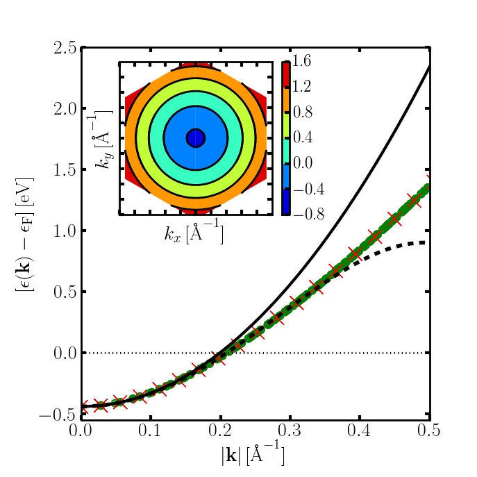
Figure 3: (Color online) Dispersion of the surface state plotted as a function of $|\mathbf{k}|$ for ${\mathbf{k}}$ sampled evenly on a 2D grid. The full (dashed) curve gives the best-fit second- (fourth-) order polynomial. The dotted line indicates the Fermi surface. The filled [green] circles, which form a thick line, indicate the calculated values, while the [red] crosses indicate those for $k_{y}=0$. The insert shows the energy contours as function of $\mathbf{k}$, with ticks having the same spacing as in the main figure.

IV Surface state in an external electrical field

The dispersion of the Shockley surface state was characterized in the previous section at zero electrical field. In this section, we present the results for a finite external electrical field.

IV.1 Wavefunctions and potential profile

Figure 1 gives intersections or contours of the variation of the surface-state density in three dimensions. Fig. 1 confirms that the surface state is mostly located between the copper layers or outside the outermost copper layer. The figure also shows that, in the in-plane direction, the density is largest close to the copper atoms. The upper panel of Fig. 4 shows the sum-projected density of the KS wavefunctions at the $\bar{\Gamma}$ point, $\rho_{i}^{{\rm KS,(}E{\rm)}}(z)$, for different external electrical fields $E$. For zero field (top line), the two wavefunctions form approximately symmetric and anti-symmetric functions as depicted by the full (green) and dashed (black) curve, respectively. That the two curves have almost equal magnitude on the left side, but not on the right, reflects the presence of numerical noise and grid sensitivities in the plane-wave DFT calculations. The lower panel of Fig. 4 shows the sum-projected density of the SL states at the ${\bar{\Gamma}}$ point, $\rho_{i}^{{\rm SL,(}E{\rm)}}(z)$, and the average potential energy as a function of $z$. The SL states differ marginally for different electrical fields; hence, we only display those for zero electrical field. These states exhibit oscillatory exponential decay into the bulk and are located solely on one side (or the other) of the slab, further validating use of the MaxLoc condition. The filled (yellow) circles indicate the location of the copper atoms. The first node of the wavefunctions coincides with the position of the top copper layer. The (laterally averaged) potential energy profiles for the three field strengths are given by surfaces of semi-transparent grey shading; thus, the light-,medium-, and dark grey areas indicate energies which are smaller than one, two, or all three of the potentials. A sharp edge between dark grey and white indicates that the potentials overlap, for example within the slab. At the left side of the slab, the finite electrical fields go outward from the surface, corresponding to a total reduction of electrons. The number of surface-state electrons are also reduced on the left side as the electrical field push the electrons toward the surface and thereby increases confinement. This raises the minimum energy $\epsilon(0)$ of the surface state, lowering $\epsilon_{F}-\epsilon(0)$. At the right side, electrons accumulate and so do the surface state electrons; they experience weakening confinement, hence a lowering of the energy which leads to an increasing value of $\epsilon_{F}-\epsilon(0)$. For large electrical fields, the surface state becomes increasingly unstable, and at some point, depending on the size of the vacuum region in the unit cell, electrons start accumulating at the dipole layer, ruining the physical picture of semi-stable surface states.

Figure 4: (Color online) The average potential profile and KS and SL surface-state densities at the $\bar{\Gamma}$ point for a Cu(111) surface in an external electrical field $\mathbf{E}$ pointing to the left, i.e., inwards to the surface at the top (at $z\approx 0$) of the slab and outwards from the surface at the bottom (at $z\approx-30\hbox{\AA}$). Thus, the force on an electron is away from the surface at the top of the slab and the minimum energy $\epsilon(0)$ of this top-surface SL state is lowered, increasing $\epsilon_{F}-\epsilon(0)$. The upper panel shows the KS surface-state densities (full and dashed) for three different strengths of E. At zero electrical field they are almost symmetric, while for larger field they almost decouple. The inserts illustrate the corresponding hybridization parameters. The lower panel shows the atom positions, filled (yellow) circles, and the decoupled SL surface states, evanescent oscillatory curves. The bottom panel also shows, by surfaces of semi-transparent grey shading, the potential profile for the three different strengths of electrical fields. Field-induced changes in the potential profile are observable only outside the outermost Cu atoms.

IV.2 Modified dispersion

Figure 5: (Color online) Calculated energy at the ${\bar{\Gamma}}$-point (upper panel) and mass (middle panel) shift for different external electrical fields. Here we take a positive value of the field strength $E$ to imply that the field $\mathbf{E}$ (the force) points away from (towards) the surface. In terms of the underlying slab calculations, Fig. 4, the positive-$E$ (negative-$E$) results characterize the behavior of the SL state at the left-most (right-most) slab surface. The filled (red) circles [(white) diamond] gives the calculated values for a 15 [12] layer slab. The black line gives the least-square fit to the calculated data. In the lower panel the relative shift in wavelength (wave vector) is given by the full (dashed) curve.

The external electrical field not only modifies the effective Fermi level $\epsilon_{F}$ of the surface state, but also influences the surface-state dispersion, expressed here in terms of a shift in the effective mass. The mass is obtained as described in the previous section. Figure 5 shows the calculated values of the surface-state energy relative to the effective Fermi level (upper panel), the effective mass (mid panel), and in the lower panel, the relative shift in the wavelength and the wave vector based on the shift in Fermi level and effective mass in the parabolic free-electron gas approximation. It shows that for the largest plotted electrical field the wavelength shifts by about $4\%$. For the upper and mid panel, the line gives the least-square fit according to linear relations:

$$\left[\epsilon_{F}-\epsilon(0)\right]_{E} = \left[\epsilon_{F}-\epsilon(0)\right]_{E=0}+A_{\epsilon}E$$ (9)

$$m^{(E)}/m_{e} = m^{(0)}/m_{e}+A_{\hat{m}}E\,,$$ (10)

where $\hat{m}$ denotes $m/m_{e}$. The parameters determined are listed in Table 3 along with the shift in the characteristic Fermi wave vector $k_{F}$ ($A_{\rm k_{F}}$) and in the wavelength $\lambda_{F}$ ($A_{\lambda_{F}}$).

Table 3: Response of the surface state to the external electrical field, obtained from fitting to the calculated dispersion. The values $A_{\epsilon},A_{\hat{m}},A_{\lambda_{F}}$, and $A_{k_{F}}$ are our results for the field derivatives of the surface-state Fermi sea level, $\epsilon_{F}-\epsilon(0)$, effective mass, Fermi wavelength, and Fermi wavevector, respectively. The value of $A_{\sigma}$ is our DFT-based determination of the fraction of overall external-field screening which originates from the surface-state behavior.

$A_{\epsilon}[{\rm e\AA}]$	-0.	146 ($\pm 0.007$)
$A_{\hat{m}}[{\rm\AA/V}]$	0.	029
$A_{k_{F}}[{\rm V}^{-1}]$	-0.	025
$A_{\lambda_{F}}[{\rm\AA}^{2}{\rm V}^{-1}]$	3.	68
$A_{\sigma}[{\rm(V\AA)^{-1}}]$	-4.	$82\cdot 10^{-3}$

The range of field strengths $E$ plotted in Fig. 5 are larger than values which are directly achievable in most experiments (but smaller than what is regularly achieved in adsorption studies, as discussed in Sec. V). In particular, in a study of the Stark shift of the surface state due to measurement by scanning tips rather than photoemission, Berndt’s groupKröger et al. (2004) found a linear decrease in $\left[\epsilon_{F}-\epsilon(0)\right]_{E}$ vs. $E$. This is true up to $E$ = 0.055 V/Å, at which there is a energy shift of magnitude $\sim$13 meV; thereafter, the rate of change increased markedly, an effect which the authors attributed to the breakdown of the tunneling regime at small tip-surface separation. We note that while the experimentally observed breakdown occurs around 0.055 V/Å for Cu(111), it occurs already at 0.008 V/Å for the more weakly bound Shockley state on Ag(111). From their graph of energy shift vs. field, we extract the mean slope to be $A_{\epsilon}\approx-0.23$ eÅ for Cu(111), comparable to our computed value in Table 3. We speculate that the larger magnitude in the experiment arises from the additional strain in lateral directions due to the non-uniform field between the STM tip and the surface.

V Discussion

V.1 Role of the surface state in screening an external field

In a metal, the electrons close to the Fermi level completely screen an external static electrical field perpendicular to the surface. The virtually identical potential profile inside the slab, for $-30{\rm\AA}<z<0$, in the lower panel of Fig. 4 for different electrical fields shows that our DFT calculations accounts for this screening. Figure 6 displays the charge density response to the external fields. The charge is induced outside the outermost copper atom, while there are small oscillations into the first two bulk layers. The response is almost identical, with opposite prefactor, at the other side of the slab. The short screening length indicates that the bulk electrons play a major role in screening the electric field.

Figure 6: (Color online) Charge transfer induced by external electrical field averaged over the in-plane directions. The upper light (cyan) [dark (black), dashed (orange)] is for $E=-0.36\,[-0.12,0.24]\,{\rm V/\AA}$.

To determine the fraction of the screening performed by the surface state compared to the bulk states, we obtain the total charge induced on the surface from Gauss’s law and the charge accumulated in the surface state with its parabolic free-electron dispersion. Gauss’s law relates the induced charge on the surface to the electrical field by $\sigma=\varepsilon_{0}E$. To obtain the charge accumulation in the surface state, we recall that 2d-electron density of states (including spin degeneracy) is $m\epsilon_{F}/\pi$ (assuming in this paragraph, for notational simplicity, that $\epsilon(0)=0$). Then the charge density due to the surface state is $\sigma_{s}=-em\epsilon_{F}/\pi$ at $T=0$, which is the appropriate temperature for comparison with standard DFT calculations. Since the mass $m$ and the Fermi-level $\epsilon_{F}$ change as an external electrical field is applied, so does the charge of the surface state. To first order in the electrical field, this shift is given by $\Delta\sigma_{s}=-\Delta(m\epsilon_{F})e/\pi=-A_{\sigma}eE/\pi+\mathcal{O}(E^{2})$, where $A_{\sigma}=\left(mA_{\epsilon}+A_{\hat{m}}\epsilon_{F}\right)$. Combining the expressions, we find the fraction of the electrical field screened by the surface state:

$$\frac{\Delta\sigma_{s}}{\sigma}=\frac{-eA_{\sigma}}{\varepsilon_{0}\pi}+\mathcal{O}(E)=0.27\,.$$ (11)

The surface state therefore plays a significant but not dominant role in the screening of the electrical field. We note that the calculated potential profile and induced charge density curves exhibit minute oscillatory variation for different fields. This observation, again, accords well with the idea that bulk electrons perform most of the screening. That screening arises predominantly from bulk electrons has several noteworthy consequences. It supports the practice of calculating interaction energies due to surface-state mediated interactionsRepp et al. (2000); Hyldgaard and Persson (2000); Hyldgaard and Einstein (2002, 2003, 2005) based solely on the changes in the energies of single-particle states, ignoring the electrostatic term in the full Harris formalism.Harris (1985) It also suggests that interactions between closely spaced adsorbates (within a few lattice spacings of each other) are dominated by the bulk states rather than the surface states. Based on a STM study Petersen et al.Petersen et al. (1998) concluded that screening of step edges at the surface was dominated by the surface states on Cu(111) an Au(111), but they also noted that screening of defects slightly below the surface is dominated by bulk electrons. The important role of the bulk electrons is also reflected in the linear dispersion of acoustic-surface plasmons on Cu(111).Silkin et al. (2005); Pohl et al. (2010)

V.2 Comparison with experiments

Table 4: Experimental results for alkali adsorbates and electric fields on the Shockley surface state on Cu and Ag (111). The ratio of effective to bare electron mass is indicated by $\hat{m}$. Unless indicated otherwise, coverages are a saturated overlayer (“1 ML”). The entries for electric fields, denoted by “E:substrate”, are those discussed in Subsection IV.2; the “adsorbed” values are for the the maximum fields before the tunneling regime breaks down (not the tabulatedKröger et al. (2004) values for $R=500M\Omega$).

System	[$\epsilon_{F}-\epsilon(0)]$ [meV]		$\hat{m}$
	clean	adsorbed	clean	adsorbed
$\lesssim\frac{1}{2}$ML Li/Cu ,		755
0.11-0.15ML Na/Cu	390	800
0.4ML K/Cu	410	755	0.41	0.36
Cs/Cu
Ar/Cu	434(2)	376(3)	0.43(1)	0.46(3)
Kr/Cu	434(2)	358(2)	0.43(1)	0.44(2)
Xe/Cu	434(2)	291(2)	0.43(1)	0.44(2)
Xe/Cu	440(10)	310(10+)	0.40(2)	0.42(3)
$\frac{1}{4}$ML Na/Cu	$\sim$340	690
C6H6/Cu	410	240	0.46	0.9
E:Cu	437(1)	450
0.17ML Na/Ag	-65	-260
Ar/Ag	62(2)	-1(3)	0.42(1)	0.46(4)
Kr/Ag	62(2)	-08(2)	0.42(1)	0.44(4)
Xe/Ag	62(2)	-52(2)	0.42(1)	0.42(6)
Xe/Ag	67	-52	ratio = 1.00(15)
E:Ag	64(1)	71

Ref Carlsson et al., 1998 indicates that the surface state shifts down with Li adsorption and disappears (into the bulk) before a half monolayer. Ref Kliewer and Berndt, 2001 Ref. Carlsson et al., 1997 Ref. Schiller et al., 2008 Ref. Forster et al., 2003 Ref. Park et al., 2000 Ref. Lindgren and Walldén, 1980 Ref. Munakata, 1999 Ref. Kröger et al., 2004 Ref Carlsson et al., 1996 Ref Wang et al., 2011 Ref. Hövel et al., 2001 Ref. Limot et al., 2003

In Table 4 we collect results for adsorption-induced shifts in $\epsilon_{F}-\epsilon(0)$, as well as changes in the effective mass and the workfunction when available, for Cu(111) and Ag(111) to provide information about the kinds of values measured in mostly-recent experiments. We have not included gold-surface-adsorbate systems because of the strong spin-orbit coupling gives rise to a Bychkov-Rashba splitting.Bychkov and Rashba (1985); LaShell et al. (1996); Simon et al. (2011) In addition, Au(111), in contrast to Cu, Ag, and other fcc (111) surfaces, reconstructs, taking on a herringbone pattern.Wöll et al. (1989); Barth et al. (1990) We note that is not always possible to fully calibrate the values in the experiments since precise coverages are rarely given. Data is typically for a monolayer (1 ML), which refers to the saturation coverage rather than one adsorbate per substrate atom. Even if this information were available, there are many other factors, discussed at the outset, which can contribute to the shift. This is true especially for non-alkali adsorbates. Alkali adsorbates invariably lower the surface band, eventually dragging it into the bulk continuum, where it becomes a resonance; often the details are not reported (for example for Cs/Cu(111)Breitholtz et al. (2007)); associated calculations are problematic due to the large unit cells needed for fractional coverage and ill-defined order. There have been recent studies, using two-photon photoemission of all the alkalis on Cu(111)Zhao et al. (2008) and on Ag(111)Wang et al. (2011); they confirm the downward shift but offer little additional quantitative information on the coverage dependence of the shifts. To address this shift quantitatively with DFT for Na/Cu(111) while keeping a manageable cell size, Caravati and TrioniCaravati and Trioni (2010) used a jellium-like model with one-dimensional Chulkov potentialChulkov et al. (1999) and found $\epsilon_{F}-\epsilon(0)$ to be colinear for coverages $\Theta$ = 0, 0.06, and 0.14, of the form $-0.303-2.2\Theta$, with a slightly smaller negative slope when $\Theta$ = 0.25 was also included. For noble-gas adsorbates, the shifts are large while the increase in effective mass is small, implying that more than just field effects are involved. In passing, we discuss a specific complication in deciphering the tabulated numbers: the lateral dipolar interaction. This effect can influence the field at other sites. Most significantly, as alkali atoms get close to each other, the direct dipolar repulsion becomes more important than the indirect, surface-state-mediated interaction. This happens when the dipole is large enough to produce a significant shift in the surface state.Fratesi et al. (2010) We note that the maximum downwards shifts possible for metallic surface states are approximatively set by the $E=0$ value of the minimum surface-state energy $\epsilon_{F}-\epsilon^{E=0}(0)$, for example, as measured in Ref. Kröger et al., 2004 and reported in Table IV (as the ‘clean’ entry in the ‘E:substrate’ rows). The maximum possible upward shift in $\epsilon^{E\neq 0}(0)$ is instead approximatively given by the difference between value of $\epsilon^{E=0}(0)$ and the energy $\varepsilon^{\rm bulk}(L)=900$meV of the bulk state at the bottom of the Cu L-gapKnapp et al. (1979); Kevan (1983) (since the overlap in energies will convert the surface state to a surface-state resonance). The maximum upward shifts of the surface state for Cu can therefore be estimated by $\epsilon^{E=0}(0)-\varepsilon^{\rm bulk}(L)\approx$ 460meV. When making precise use of the band shifts, one must take into account the temperature, as discussed in detail for the (111) faces of the three noble metals by Paniago et al.Paniago et al. (1995) In particular, they show $\epsilon_{F}-\epsilon^{E=0}(0)$ = $-$(75 $\pm$ 5) meV +(0.17 meV/K) $T$ for Ag(111). There is a small increase also in $\hat{m}$, from 0.43 $\pm$ 0.04 at 65 K to 0.45 $\pm$ 0.04 at 294 K. For Cu(111) the increase is comparable, with linear coefficient (0.18 $\pm$ 0.01) meV/K. Overall, it is noteworthy that shifts far larger than those reported at the end of Subsection IV.2 are seen. The adsorption-induced shifts are indeed larger than the shifts of 50 meV which formed the abscissa limits in Fig. 5. Hence, the range of field strengths investigated in our study are physically sensible.

V.3 Decoupling method for adsorbed molecules

Our study of response to an external field has been aided by the decoupling method described and tested in Section II. This method can also be used to study shift in surface-state energy produced by an adsorbed molecule or atom. This requires that the two KS states corresponding to the SL states do not hybridize with other bulk or molecular KS states. For systems with inversion symmetry in the plane (in terms of the basis vectors), like benzene on Cu(111),Berland et al. (2009) we only need to decouple the states using an O(2) rotation. As a test case, we consider benzene on Cu(111) in a 3$\times$3 periodic unit cell and a 6 layer slab. Using DFT with the vdW-DF2 functional to capture the non-local correlation essential to the binding of this system,Lee et al. (2010) we determine a binding separation of $3.5{\rm\AA}$, and a binding energy of 0.48 eV. Except for the use of vdW-DF2, the details of this calculation are the same as in our previously reported calculation with vdW-DF1.Berland et al. (2009) After decoupling the two KS states, we find a coupling of $\Omega=320$meV and a detuning of $W=16{\rm meV}$. Since for the adsorbed-molecule case only one of the surfaces is perturbed, the energy difference between the decoupled states $2W=32{\rm meV}$ equals the shift in surface state energy. In this calculation, the decoupling method enabled us to extract the shift in surface state energy in a traditional slab calculation using far fewer layers than what would be required for the KS to fully decouple because of the (weakly) broken symmetry. We have also used the method to study the surface shift induced by adsorbed anthraquinone chains on Cu(111) for varying coverages.Wyrick et al. (2011)

VI Conclusions

Using DFT calculations, we have shown that an electric field perpendicular to a metal surface with a metallic Shockley surface state linearly shifts the bottom of this state (relative to the Fermi energy) for physically plausible field strengths. We have computed the value of the linear proportionality constant, as well as that associated with the field-induced change in the curvature of the dispersion relation, that is, in the effective mass. The decoupling method presented here should be useful when studying the response in the surface-state dispersion to a perturbation that does not destroy the surface-state character. It is, for example, relevant for a study of the surface response arising from organic overlayers weakly coupled to the surface or dilute overlayers of chemisorbed atoms. More generally, the MaxLoc analysis could be useful for decoupling states which arise at different spatial locations and which hybridize under the asumption that an infinite time is available to create the coupling. The characterization of the coupling in such systems can be used to calculate tunneling rates and oscillation frequencies. It is hard to overemphasize the significance of acquiring the ability to control the Fermi wavelength in order to manipulate and engineer surface structures determined by interactions mediated by surface states. With a strong enough field, one could in principle manipulate channels in a manner reminiscent of Repp’s resonatorNegulyaev et al. (2008) and so dynamically direct an atom flow on surface.

VII Acknowledgement

The authors thank the Swedish National Infrastructure for Computing (SNIC) for access and for KB’s participation in the graduate school NGSSC. The work at Chalmers was supported by the Swedish research Council (Vetenskapsrådet VR) under 621-2008-4346 and by VINNOVA. Work at U. of Maryland was supported by NSF Grant CHE 07-50334 and by NSF-MRSEC Grant DMR 05-20471 and ancillary support from the Center for Nanophysics and Advanced Materials (CNAM) and a DOE CMCSN grant.

References

- Shockley (1939) W. Shockley, Phys. Rev. 56, 317 (1939).
- bk: (a) S. G. Davison and M. Stȩślicka, Basic Theory of Surface States, (Oxford University Press, Oxford, 1996).
- bk: (b) S.D. Kevan, ”Surface States on Metal Surfaces,” in Electronic Structure, Handbook of Surface Sci., vol. 2 (Elsevier, Amsterdam, 2000), p. 433.
- (4) P. Han and P. S. Weiss, Electronic Substrate-Mediated Interactions, Surface Sci. Reports, submitted.
- Gartland and Slagsvold (1975) P. O. Gartland and B. J. Slagsvold, Phys. Rev. B 12, 4047 (1975).
- Reinert et al. (2001) F. Reinert, G. Nicolay, S. Schmidt, D. Ehm, and S. Hüfner, Phys. Rev. B 63, 115415 (2001).
- Crommie et al. (1993) M. F. Crommie, C. P. Lutz, and D. M. Eigler, Science 262, 218 (1993).
- Heller et al. (1994) E. J. Heller, M. F. Crommie, C. P. Lutz, and D. M. Eigler, Nature (London) 369, 464 (1994).
- Crommie et al. (1995) M. F. Crommie, C. P. Lutz, D. M. Eigler, and E. J. Heller, Surface Review and Letters 2, 127 (1995).
- Fiete and Heller (2003) G. A. Fiete and E. J. Heller, Rev. Mod. Phys. 75, 933 (2003).
- Hyldgaard and Persson (2000) P. Hyldgaard and M. Persson, J. Phys.: Condens. Mat. 12, L13 (2000).
- Repp et al. (2000) J. Repp, F. Moresco, G. Meyer, K.-H. Rieder, P. Hyldgaard, and M. Persson, Phys. Rev. Lett. 85, 2981 (2000).
- Hyldgaard and Einstein (2002) P. Hyldgaard and T. L. Einstein, EPL (Europhysics Letters) 59, 265 (2002).
- bk: (c) T.L. Einstein, ”Interactions between Adsorbed Particles,” in Physical Structure of Solid Surfaces, Handbook of Surface Sci., vol. 1, edited by W.N. Unertl (Elsevier, Amsterdam, 1996), p. 577.
- Hyldgaard and Einstein (2003) P. Hyldgaard and T. L. Einstein, Surf. Sci. 532, 600 (2003).
- Stepanyuk et al. (2003) V. S. Stepanyuk, A. N. Baranov, D. V. Tsivlin, W. Hergert, P. Bruno, N. Knorr, M. A. Schneider, and K. Kern, Phys. Rev. B 68, 205410 (2003).
- Hyldgaard and Einstein (2005) P. Hyldgaard and T. L. Einstein, J. Crystal Growth 275, e1637 (2005).
- Nanayakkara et al. (2007) S. U. Nanayakkara, E. C. H. Sykes, L. C. Fernández-Torres, M. M. Blake, and P. S. Weiss, Phys. Rev. Lett. 98, 206108 (2007).
- Chen and Smith (1989) C. T. Chen and N. V. Smith, Phys. Rev. B 40, 7487 (1989).
- Dudde et al. (1990) R. Dudde, K. H. Frank, and B. Reihl, Phys. Rev. B 41, 4897 (1990).
- Schiller et al. (2008) F. Schiller, M. Corso, M. Urdanpilleta, T. Ohta, A. Bostwick, J. L. McChesney, E. Rotenberg, and J. E. Ortega, Phys. Rev. B 77, 153410 (2008).
- Fischer et al. (1994) N. Fischer, S. Schuppler, T. Fauster, and W. Steinmann, Surf. Sci. 314, 89 (1994).
- Breitholtz et al. (2007) M. Breitholtz, V. Chis, B. Hellsing, S.-Å. Lindgren, and L. Walldén, Phys. Rev. B 75, 155403 (2007).
- Chis et al. (2007) V. Chis, S. Caravati, G. Butti, M. I. Trioni, P. Cabrera-Sanfelix, A. Arnau, and B. Hellsing, Phys. Rev. B 76, 153404 (2007).
- Carlsson et al. (1997) A. Carlsson, B. Hellsing, S.-Å. Lindgren, and L. Walldén, Phys. Rev. B 56, 1593 (1997).
- Momma and Izumi (2008) K. Momma and F. Izumi, J. Applied Crystallography 41, 653 (2008).
- Lindell et al. (2005) L. Lindell, M. P. de Jong, W. Osikowicz, R. Lazzaroni, M. Berggren, W. R. Salaneck, and X. Crispin, J. Chem. Phys. 122, 084712 (2005).
- Fratesi et al. (2010) G. Fratesi, A. Pace, and G. P. Brivio, J. Phys.: Condens. Mat. 22, 304005 (2010).
- Limot et al. (2003) L. Limot, T. Maroutian, P. Johansson, and R. Berndt, Phys. Rev. Lett. 91, 196801 (2003).
- Kröger et al. (2004) J. Kröger, L. Limot, H. Jensen, R. Berndt, and P. Johansson, Phys. Rev. B 70, 033401 (2004).
- Lang and Kohn (1970) N. D. Lang and W. Kohn, Phys. Rev. B 1, 4555 (1970).
- Weber and Liebsch (1987) M. Weber and A. Liebsch, Phys. Rev. B 35, 7411 (1987).
- Chizmeshya and Zaremba (1988) A. Chizmeshya and E. Zaremba, Phys. Rev. B 37, 2805 (1988).
- Kiejna (1995) A. Kiejna, Surf. Sci. 331-333, 1167 (1995).
- Hult et al. (1996) E. Hult, Y. Andersson, B. I. Lundqvist, and D. C. Langreth, Phys. Rev. Lett. 77, 2029 (1996).
- Feibelman (2001) P. J. Feibelman, Phys. Rev. B 64, 125403 (2001).
- Inglesfield (1991) J. E. Inglesfield, Phil. Trans.: Phys. Sci. & Eng. 334, 527 (1991).
- Negulyaev et al. (2011) N. N. Negulyaev, V. S. Stepanyuk, W. Hergert, and J. Kirschner, Phys. Rev. Lett. 106, 037202 (2011).
- Achilli et al. (2007) S. Achilli, S. Caravati, and M. I. Trioni, Surf. Sci. 601, 4048 (2007).
- (40) E. M. Lifshitz, Zh. Eksp. Teor. Fiz. 29, 94 (1955) [Sov. Phys.-JETP 2, 73 (1956)].
- Zaremba and Kohn (1976) E. Zaremba and W. Kohn, Phys. Rev. B 13, 2270 (1976).
- Apell (1981) P. Apell, Physica Scripta 24, 795 (1981).
- Persson and Apell (1983) B. N. J. Persson and P. Apell, Phys. Rev. B 27, 6058 (1983).
- Persson and Zaremba (1984) B. N. J. Persson and E. Zaremba, Phys. Rev. B 30, 5669 (1984).
- Liebsch (1987) A. Liebsch, Phys. Rev. B 36, 7378 (1987).
- Rydberg et al. (2000) H. Rydberg, B. I. Lundqvist, D. C. Langreth, and M. Dion, Phys. Rev. B 62, 6997 (2000).
- Andersson et al. (1998) Y. Andersson, E. Hult, H. Rydberg, B. I. Lundqvist, and D. C. Langreth, Solid State Commun. 106, 235 (1998).
- Hult et al. (1999) E. Hult, H. Rydberg, B. I. Lundqvist, and D. C. Langreth, Phys. Rev. B 59, 4708 (1999).
- Hult et al. (2001) E. Hult, P. Hyldgaard, J. Rossmeisl, and B. I. Lundqvist, Phys. Rev. B 64, 195414 (2001).
- Dion et al. (2004) M. Dion, H. Rydberg, E. Schröder, D. C. Langreth, and B. I. Lundqvist, Phys. Rev. Lett. 92, 246401 (2004).
- Thonhauser et al. (2007) T. Thonhauser, V. R. Cooper, S. Li, A. Puzder, P. Hyldgaard, and D. C. Langreth, Phys. Rev. B 76, 125112 (2007).
- Lee et al. (2010) K. Lee, E. D. Murray, L. Kong, B. I. Lundqvist, and D. C. Langreth, Phys. Rev. B 82, 081101(R) (2010).
- Rydberg et al. (2003) H. Rydberg, M. Dion, N. Jacobson, E. Schröder, P. Hyldgaard, S. I. Simak, D. C. Langreth, and B. I. Lundqvist, Phys. Rev. Lett. 91, 126402 (2003).
- Zaremba and Kohn (1977) E. Zaremba and W. Kohn, Phys. Rev. B 15, 1769 (1977).
- Nordlander and Harris (1984) P. Nordlander and J. Harris, J. Phys. C: Solid State Phys. 17, 1141 (1984).
- Andersson and Persson (1993) S. Andersson and M. Persson, Phys. Rev. B 48, 5685 (1993).
- Lee et al. (2011) K. Lee, A. K. Kelkkanen, K. Berland, S. Andersson, D. C. Langreth, E. Schröder, B. I. Lundqvist, and P. Hyldgaard, Phys. Rev. B 84, 193408 (2011).
- Kleis et al. (2008) J. Kleis, E. Schröder, and P. Hyldgaard, Phys. Rev. B 77, 205422 (2008).
- Berland and Hyldgaard (2010) K. Berland and P. Hyldgaard, J. Chem. Phys. 132, 134705 (2010).
- Berland et al. (2011) K. Berland, Ø. Borck, and P. Hyldgaard, Comp. Phys. Comm. 182, 1800 (2011).
- Pawin et al. (2006) G. Pawin, K. L. Wong, K.-Y. Kwon, and L. Bartels, Science 313, 961 (2006).
- Kim and Einstein (2011) K. Kim and T. L. Einstein, Phys. Rev. B 83, 245414 (2011).
- Wyrick et al. (2011) J. Wyrick, D.-H. Kim, D. Sun, Z. Cheng, W. Lu, Y. Zhu, K. Berland, Y. S. Kim, E. Rotenberg, M. Luo, et al., Nano Lett. 11, 2944 (2011).
- Cheng et al. (2010) Z. Cheng, M. Luo, J. Wyrick, D. Sun, D. Kim, Y. Zhu, W. Lu, K. Kim, T. L. Einstein, and L. Bartels, Nano Lett. 10, 3700 (2010).
- Inglesfield (1981) J. E. Inglesfield, J. Phys. C 14, 3795 (1981).
- Nekovee and Inglesfield (1992) M. Nekovee and J. Inglesfield, EPL 19, 535 (1992).
- Szunyogh et al. (1994) L. Szunyogh, B. Újfalussy, P. Weinberger, and J. Kollár, Phys. Rev. B 49, 2721 (1994).
- Szunyogh et al. (1995) L. Szunyogh, B. Újfalussy, and P. Weinberger, Phys. Rev. B 51, 9552 (1995).
- Ishida (2001) H. Ishida, Phys. Rev. B 63, 165409 (2001).
- Lazarovits et al. (2002) B. Lazarovits, L. Szunyogh, and P. Weinberger, Phys. Rev. B 65, 104441 (2002).
- Butti et al. (2005) G. Butti, S. Caravati, G. P. Brivio, M. I. Trioni, and H. Ishida, Phys. Rev. B 72, 125402 (2005).
- Eguiluz et al. (1992) A. G. Eguiluz, M. Heinrichsmeier, A. Fleszar, and W. Hanke, Phys. Rev. Lett. 68, 1359 (1992).
- Sau et al. (2008) J. D. Sau, J. B. Neaton, H. J. Choi, S. G. Louie, and M. L. Cohen, Phys. Rev. Lett. 101, 026804 (2008).
- Kokalj and Causà (1999) A. Kokalj and M. Causà, J. Phys.: Condens. Mat. 11, 7463 (1999).
- Carlsson and Hellsing (2000) J. M. Carlsson and B. Hellsing, Phys. Rev. B 61, 13973 (2000).
- Fichthorn and Scheffler (2000) K. A. Fichthorn and M. Scheffler, Phys. Rev. Lett. 84, 5371 (2000).
- Bogicevic et al. (2000) A. Bogicevic, S. Ovesson, P. Hyldgaard, B. I. Lundqvist, H. Brune, and D. R. Jennison, Phys. Rev. Lett. 85, 1910 (2000).
- Fölsch et al. (2004) S. Fölsch, P. Hyldgaard, R. Koch, and K. H. Ploog, Phys. Rev. Lett. 92, 056803 (2004).
- Chis and Hellsing (2004) V. Chis and B. Hellsing, Phys. Rev. Lett. 93, 226103 (2004).
- Luo and Fichthorn (2005) W. Luo and K. A. Fichthorn, Phys. Rev. B 72, 115433 (2005).
- Da Silva et al. (2006) J. L. F. Da Silva, C. Barreteau, K. Schroeder, and S. Blügel, Phys. Rev. B 73, 125402 (2006).
- Yu et al. (2006) D. Yu, M. Scheffler, and M. Persson, Phys. Rev. B 74, 113401 (2006).
- Forster et al. (2007) F. Forster, A. Bendounan, F. Reinert, V. Grigoryan, and M. Springborg, Surf. Sci. 601, 5595 (2007).
- Wong et al. (2007) K. L. Wong, G. Pawin, K.-Y. Kwon, X. Lin, T. Jiao, U. Solanki, R. H. J. Fawcett, L. Bartels, S. Stolbov, and T. S. Rahman, Science 315, 1391 (2007).
- Howe et al. (2010) J. D. Howe, P. Bhopale, Y. Tiwary, and K. A. Fichthorn, Phys. Rev. B 81, 121410 (2010).
- Hayat et al. (2010) S. S. Hayat, M. Alcántara Ortigoza, M. A. Choudhry, and T. S. Rahman, Phys. Rev. B 82, 085405 (2010).
- Bjork et al. (2010) J. Bjork, M. Matena, M. S. Dyer, M. Enache, J. Lobo-Checa, L. H. Gade, T. A. Jung, M. Stohr, and M. Persson, Phys. Chem. Chem. Phys. 12, 8815 (2010).
- Dyer and Persson (2010) M. S. Dyer and M. Persson, New J. Phys. 12, 063014 (2010).
- Perdew et al. (1996) J. P. Perdew, K. Burke, and M. Ernzerhof, Phys. Rev. Lett. 77, 3865 (1996).
- (90) Open source code DACAPO, http://www.fysik.dtu.dk/CAMPOS/.
- Com (a) The corresponding cutoff for the density was set to 500 eV.
- Harris (1985) J. Harris, Phys. Rev. B 31, 1770 (1985).
- Com (b) In preliminary low-accurcy calculations, the max force was 0.055 for the smallest electrical field, and 0.057 for the largest. For a high accurcay calculations at zero electical field, the max force was 0.042, smaller than the standard limit of 0.05. Thus we do not include relaxations as they are prone to introduce small kinks in the curves.
- Bengtsson (1999) L. Bengtsson, Phys. Rev. B 59, 12301 (1999).
- Neugebauer and Scheffler (1992) J. Neugebauer and M. Scheffler, Phys. Rev. B 46, 16067 (1992).
- Kohn (1959) W. Kohn, Phys. Rev. 115, 809 (1959).
- Marzari and Vanderbilt (1997) N. Marzari and D. Vanderbilt, Phys. Rev. B 56, 12847 (1997).
- Berland et al. (2009) K. Berland, T. L. Einstein, and P. Hyldgaard, Phys. Rev. B 80, 155431 (2009).
- Jeandupeux et al. (1999) O. Jeandupeux, L. Bürgi, A. Hirstein, H. Brune, and K. Kern, Phys. Rev. B 59, 15926 (1999).
- Kevan and Gaylord (1987) S. D. Kevan and R. H. Gaylord, Phys. Rev. B 36, 5809 (1987).
- Courths et al. (2001) R. Courths, M. Lau, T. Scheunemann, H. Gollisch, and R. Feder, Phys. Rev. B 63, 195110 (2001).
- Bürgi et al. (2000) L. Bürgi, L. Petersen, H. Brune, and K. Kern, Surf. Sci. 447, L157 (2000).
- (103) The effect of this anisotropy on the asymptotic interaction is treated in P. N Patronice and T. L. Einstein, submitted to Phys. Rev. B.
- Becker et al. (2006) M. Becker, S. Crampin, and R. Berndt, Phys. Rev. B 73, 081402 (2006).
- Petersen et al. (1998) L. Petersen, P. Laitenberger, E. Lægsgaard, and F. Besenbacher, Phys. Rev. B 58, 7361 (1998).
- Silkin et al. (2005) V. M. Silkin, J. M. Pitarke, E. V. Chulkov, and P. M. Echenique, Phys. Rev. B 72, 115435 (2005).
- Pohl et al. (2010) K. Pohl, B. Diaconescu, G. Vercelli, L. Vattuone, V. M. Silkin, E. V. Chulkov, P. M. Echenique, and M. Rocca, Europhys. Lett. 90, 57006 (2010).
- Carlsson et al. (1998) A. Carlsson, D. Claesson, G. Katrich, S.-Å. Lindgren, and L. Walldén, Phys. Rev. B 57, 13192 (1998).
- Kliewer and Berndt (2001) J. Kliewer and R. Berndt, Phys. Rev. B 65, 035412 (2001).
- Forster et al. (2003) F. Forster, G. Nicolay, F. Reinert, D. Ehm, S. Schmidt, and S. Hüfner, Surf. Sci. 532-535, 160 (2003).
- Park et al. (2000) J.-Y. Park, U. D. Ham, S.-J. Kahng, Y. Kuk, K. Miyake, K. Hata, and H. Shigekawa, Phys. Rev. B 62, R16341 (2000).
- Lindgren and Walldén (1980) S.-Å. Lindgren and L. Walldén, Sol. State Comm. 34, 671 (1980).
- Munakata (1999) T. Munakata, J. Chem. Phys. 110, 2736 (1999).
- Carlsson et al. (1996) A. Carlsson, D. Claesson, S.-Å. Lindgren, and L. Walldén, Phys. Rev. Lett. 77, 346 (1996).
- Wang et al. (2011) L.-M. Wang, V. Sametoglu, A. Winkelmann, J. Zhao, and H. Petek, J.Phys. Chem. A 115, 9479 (2011).
- Hövel et al. (2001) H. Hövel, B. Grimm, and B. Reihl, Surf. Sci. 477, 43 (2001).
- Bychkov and Rashba (1985) Y. Bychkov and E. Rashba, JETP Lett. 78 (1985).
- LaShell et al. (1996) S. LaShell, B. A. McDougall, and E. Jensen, Phys. Rev. Lett. 77, 3419 (1996).
- Simon et al. (2011) E. Simon, B. Újfalussy, B. Lazarovits, A. Szilva, L. Szunyogh, and G. M. Stocks, Phys. Rev. B 83, 224416 (2011).
- Wöll et al. (1989) C. Wöll, S. Chiang, R. J. Wilson, and P. H. Lippel, Phys. Rev. B 39, 7988 (1989).
- Barth et al. (1990) J. V. Barth, H. Brune, G. Ertl, and R. J. Behm, Phys. Rev. B 42, 9307 (1990).
- Zhao et al. (2008) J. Zhao, N. Pontius, A. Winkelmann, V. Sametoglu, A. Kubo, A. G. Borisov, D. Sánchez-Portal, V. M. Silkin, E. V. Chulkov, P. M. Echenique, et al., Phys. Rev. B 78, 085419 (2008).
- Caravati and Trioni (2010) S. Caravati and M. I. Trioni, Eur. Phys. J. B 75, 101 (2010).
- Chulkov et al. (1999) E. Chulkov, V. Silkin, and P. Echenique, Surf. Sci. 437, 330 (1999).
- Knapp et al. (1979) J. A. Knapp, F. J. Himpsel, and D. E. Eastman, Phys. Rev. B 19, 4952 (1979).
- Kevan (1983) S. D. Kevan, Phys. Rev. Lett. 50, 526 (1983).
- Paniago et al. (1995) R. Paniago, R. Matzdorf, G. Meister, and A. Goldmann, Surf. Sci. 336, 113 (1995).
- Negulyaev et al. (2008) N. N. Negulyaev, V. S. Stepanyuk, L. Niebergall, P. Bruno, W. Hergert, J. Repp, K.-H. Rieder, and G. Meyer, Phys. Rev. Lett. 101, 226601 (2008).