Thermodynamics of a Bardeen black hole in noncommutative space

Abstract

In this paper, we examine the effects of space noncommutativity on the thermodynamics of a Bardeen charged regular black hole. For a suitable choice of sets of parameters, the behavior of the singularity, horizon, mass function, black hole mass, temperature, entropy and its differential, area and energy distribution of the Bardeen solution have been discussed graphically for both noncommutative and commutative spaces. Graphs show that the commutative coordinates extrapolate all such quantities (except temperature) for a given set of parameters. It is interesting to mention here that these sets of parameters provide the singularity (essential for $r_{h}>0$) and horizon ($f(r_{h})=0$ for $r_{h}>0$) for the black hole solution in noncommutative space, while for commutative space no such quantity exists.

Keywords: Regular black hole; Noncommutative space; Thermodynamics.
PACS: 04.70.Dy; 04.70.Bw; 11.25.-w

1 Introduction

It is well known that the classical theory of relativity breaks down at Planck’s scale, $l_{p}$, where quantum gravitational effects become important. To solve this problem, it is convenient to alter Riemannian structure of space-time by some mathematical model. As in relativistic physics, gravity distorts the geometry of space-time; similarly, quantum gravity quantizes space-time. According to von Neumann, the geometrical properties of quantum mechanics are described as ”pointless structure”, which is known as ”noncommutative geometry”. Noncommutative geometry helps to handle space-time structure at very short distances [1].

Space-time noncommutativity is based on quantum mechanics. The replacement of canonical position $x^{i}$ and momentum variables $p_{j}$ with corresponding Hermitian operators, $\hat{x}^{i},~{}\hat{p}_{j}$, defines the quantum phase space that obeys Heisenberg commutation relations

$$[\hat{x}^{i},\hat{p}_{j}]=\iota\hbar\delta^{i}_{j}\quad i,j=1,2,3$$ (1)

The limit $\hbar\longrightarrow 0$ recovers an ordinary space. A noncommutative space can be realized by the coordinate operators, $\hat{x}_{i}$, satisfying the commutation relations

$$[\hat{x}^{i},\hat{x}^{j}]=\iota\theta^{ij}$$ (2)

where the noncommutative parameter $\theta^{ij}$ is a constant, real valued, antisymmetric tensor, and has dimensions of (length)² [2]. The tensor $\theta^{ij}$ is generally assumed to depend on space-time coordinates and momenta.

The space-time quantization arises in the following two problems. The first is the renormalization problem, and the second is quantum gravity. The model of quantum space-time must satisfy the following canonical commutation relations in noncommutative space (with $\hbar=1$) [1]:

$$[\hat{x}_{i},\hat{x}_{j}]=\iota\theta_{ij}\quad[\hat{x}_{i},\hat{p}_{j}]=\iota\delta_{ij}\quad[\hat{p}_{i},\hat{p}_{j}]=0$$ (3)

with

$$\theta_{ij}\theta^{ij}=0\quad\epsilon_{ijkl}\theta^{ij}\theta^{kl}=-8l^{4}_{p}$$ (4)

The replacement of the usual multiplication of fields with the $\star$-product provides the formulation of noncommutative field theories from commutative field theories [3]. The $\star$-product is defined in terms of $\theta_{ij}$ as follows [4]:

$$(f\star g)(x)=\exp\left(\frac{\iota}{2}\theta^{ij}\frac{\partial}{\partial x^{i}}\frac{\partial}{\partial y^{j}}\right)f(x)g(y)|_{x=y}$$ (5)

where $f$ and $g$ are infinitely differentiable arbitrary functions.

Myung and Yoon [5] found a three-dimensional new regular black hole with two horizons by introducing an anisotropic perfect fluid inspired by a four-dimensional noncommutative black hole. They compared the thermodynamics of this black hole with that of a nonrotating Ba$\tilde{n}$ados-Teitelboim-Zanelli (BTZ) black hole. Tejeiro and Larranaga [6] investigated a new rotating regular black hole and analyzed its thermodynamics. The results were compared with those of a rotating BTZ solution. Nicolini et al. [7] studied the effects of noncommutativity on the terminal phase of the Schwarzschild black hole evaporation. Nozari and Fazlpour [8, 9] explored the behavior of noncommutative space and the generalized uncertainty principle on the thermodynamics of a radiating Schwarzschild black hole. They also considered the effects of space noncommutativity on the thermodynamics of a Reissner-Nordstr$\ddot{o}$m (RN) black hole. Nozari and Mehdipour [10] explored space noncommutativity by generalizing the RN black hole in dD space-time and also discussed its thermodynamics. Ansoldi et al. [11] found a noncommutative geometry inspired solution of the Einstein-Maxwell field equations describing a variety of charged self-gravitating objects. Spallucci et al. [12] obtained a noncommutative solution to the field equations in higher dimensions.

Nasseri [13] investigated the effects of noncommutative spaces on the horizon, the area spectrum, and Hawking temperature of the Schwarzschild black hole. Sadeghi [14] studied noncommutative spaces in a two-dimensional black hole. He obtained the event horizon in noncommutative space up to second-order perturbation and a lower limit for the noncommutativity parameter. Also, Sadeghi and Setare [15] performed the noncommutative corrections to the behavior of a BTZ black hole. Alavi [4] investigated the parameters of a noncommutative RN black hole. He also studied the stability of the black hole and found an upper bound for the noncommutativity parameter, $\theta$.

This paper is devoted to investigating the behavior of the Bardeen charged regular black hole solution in noncommutative space. The thermodynamical quantities in this noncommutative space are studied. We compute quantities like singularity, horizon, mass function, black hole mass, Hawking temperature, entropy and its differential, area and energy distribution in noncommutative space and compare their behaviors in commutative and noncommutative spaces graphically.

In Sect. 2, we propose the usual Bardeen black hole in noncommutative space. Also, we analyze graphically the effects of space noncommutativity and commutativity on the singularity and horizon of a given regular black hole. Section 3 describes graphical behavior of space noncommutativity and commutativity of the thermodynamical quantities. Finally, we summarize the results in the last section.

2 Space noncommutativity

The Bardeen model [16] was proposed some years ago as a regular black hole obeying the weak energy condition. The metric for the Bardeen model (with $G=1$) is given by

$${ds}^{2}=\left(1-\frac{2M}{r}\right){dt}^{2}-\frac{{dr}^{2}}{\left(1-\frac{2M}{r}\right)}-{r^{2}}({d\theta}^{2}+\sin^{2}\theta{d\phi}^{2})$$ (6)

where

$$M=M(r)=\frac{mr^{3}}{(r^{2}+e^{2})^{\frac{3}{2}}}$$ (7)

is a mass function. This solution is a self-gravitating magnetic monopole with charge $e$ of nonlinear electrodynamic source and exhibits black hole behavior for $e^{2}\leq 16m^{2}/27$. For $e=0$, the solution reduces to the Schwarzschild space-time.

The spherical event horizons, $r_{h}$, are given by the roots of the equation ($g_{tt}=0$)

$$r_{h}=2M(r_{h})$$

Substituting the value of $M$, we get

$$1-\frac{2mr^{2}_{h}}{(r_{h}^{2}+e^{2})^{\frac{3}{2}}}=0$$ (8)

We introduce the following metric for the Bardeen black hole in noncommutative space [13]:

$${ds}^{2}=\left(1-\frac{2M}{\sqrt{\hat{r}\hat{r}}}\right){dt}^{2}-\frac{d\hat{r}d\hat{r}}{\left(1-\frac{2M}{\sqrt{\hat{r}\hat{r}}}\right)}-{\hat{r}\hat{r}}({d\theta}^{2}+\sin^{2}\theta{d\phi}^{2})$$ (9)

where $\hat{r}$ satisfies (3). The event horizon, $\hat{r}_{h}$, of the space-time (9) in noncommutative space satisfies the following condition:

$$1-\frac{2m\hat{r}_{h}\hat{r}_{h}}{(\hat{r}_{h}\hat{r}_{h}+e^{2})^{\frac{3}{2}}}=0$$ (10)

The $\star$-product (5) between two fields in noncommutative phase space can be replaced by a shift, called Bopp’s shift, and can be defined as [17]

$$x_{i}=\hat{x}_{i}+\frac{1}{2}\theta_{ij}\hat{p}_{j}\quad p_{i}=\hat{p}_{i}$$ (11)

where $x_{i}$ and $p_{i}$ satisfy the usual (commutative) commutation algebra

$$[x_{i},x_{j}]=0\quad[x_{i},p_{j}]=i\delta_{ij}\quad[p_{i},p_{j}]=0$$ (12)

Thus the effects of space-space noncommutativity can be calculated in commutative space. When we apply transformation (11) to line element (9), this turns out to be in terms of the position and momentum variables of commutative phase space. Using coordinate transformation (11) from $\hat{r}_{h}$ to $r_{i}$, (10) takes the following form:

$$1-\frac{2m(r_{i}-\frac{\theta_{ij}p_{j}}{2\hbar})(r_{i}-\frac{\theta_{ik}p_{k}}{2\hbar})}{\left[(r_{i}-\frac{\theta_{ij}p_{j}}{2\hbar})(r_{i}-\frac{\theta_{ik}p_{k}}{2\hbar})+e^{2}\right]^{\frac{3}{2}}}=0$$ (13)

This leads to the relations

$$1-\frac{2m}{r}-\frac{1}{r^{3}}\left({mr_{i}\theta_{ij}p_{j}}-{3me^{2}}\right)-\frac{3me^{2}r_{i}\theta_{ij}p_{j}}{r^{5}}+\ldots=0$$ (14)

or

$$1-\frac{2m}{r}-\frac{1}{r^{3}}\left(\frac{m\textbf{L}.\theta}{2}-3me^{2}\right)-\frac{3me^{2}\textbf{L}.\theta}{2r^{5}}+\ldots=0$$ (15)

where $\theta_{ij}=(1/2)\epsilon_{ijk}\theta_{k}$ and $\textbf{L}=\textbf{r}\times\textbf{p}$ is the angular momentum. If we set $\theta_{3}=\theta$ and assume that all the remaining components of $\theta$ vanish (which can be done by rotation or redefinition of the coordinates), then $\textbf{L}.\theta=L_{z}\theta$. In this case, (15) takes the form

$$r^{5}-2mr^{4}-r^{2}\left(\frac{mL_{z}\theta}{2}-3me^{2}\right)-\frac{3me^{2}L_{z}\theta}{2}=0$$ (16)

Table 1. For a singularity, the behavior of $f(r_{h})$ with sets of parameters.

Color	$m$	$L_{z}\theta$	$e$
Orange	$.00098755$	$.00001$	500.5
Blue	$.55$	$-1$	.12
Purple	$.01$	$-150$	.15
Grey	$.1$	$-.05$	1

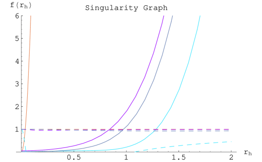
Figure 1: Horizon function, $f(r_{h})$, versus horizon radius, $r_{h}$: the solid lines represent singularity in noncommutative space for different sets of parameters given in Table 1. The dashed lines do not represent singularity in commutative space for the same sets of parameters.

In Fig. 1, it is clear that $f(r_{h})\longrightarrow\infty$ for $r_{h}>0$ with the sets of parameters given in Table 1 (for solid lines). This is because the noncommutative parameter $\theta$ is nonzero in this case. The dashed lines imply that $f(r_{h})\longrightarrow 1$ for $r_{h}=0$ with the same sets of parameters. This shows that for the commutative case there is no singularity and curves extrapolate the distance function.

Table 2. For the horizon, the behavior of $f(r_{h})$ with sets of parameters.

Color	$m$	$L_{z}\theta$	$e$
Red	$.1$	$-.009$	.9
Blue	$.0002$	$1$	3.5
Green	$.125$	$1.15$	1.5
Black	$.1$	$.0005$	.2

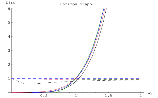
Figure 2: Horizon function, $f(r_{h})$, versus horizon radius, $r_{h}$: the four solid curves represent the horizon for the Bardeen black hole in noncommutative space with different sets of parameters given in Table 2. The dashed lines do not represent the horizon for the Bardeen black hole in commutative space with the same sets of parameters.

In Fig. 2, all four solid curves represent horizons corresponding to Bardeen solution (9) in noncommutative space with the choice of parameters given in Table 2. The dashed curves for the commutative case with the same sets of parameters indicate that there is no curve for which $f(r_{h})=0$ with nonzero horizon radius, $r_{h}\neq 0$. Here, distances also extrapolate. Thus, each of these curves does not have a meaning similar to $r=2M$ with $M=mr^{3}/(r^{2}+e^{2})^{3/2}$ in the case of the usual Bardeen solution.

3 Thermodynamics

This section is devoted to investigating graphically the behavior of thermodynamical quantities in noncommutative space. For this purpose, we choose sets of parameters given in Table 2 with horizon radii that provide four curves representing a function of horizon radius. We investigate the effects of noncommutativity on the thermodynamical quantities (mass function, black hole mass, temperature, entropy and its differential, area and energy distribution). The mass function for the Bardeen model in commutative space is given by (7), while for $\hbar=1$, its form in noncommutative space can be written as

$$\hat{M}=m\left(1-\frac{3e^{2}}{2r_{h}^{2}}+\frac{9e^{2}{L_{z}\theta}}{8r_{h}^{4}}\right)$$ (17)

The mass of the Bardeen regular black hole (8) is given by

$$m=\frac{(r_{h}^{2}+e^{2})^{\frac{3}{2}}}{2{r_{h}^{2}}}$$ (18)

while in noncommutative space, it turns out to be

$$\hat{m}=\frac{r_{h}}{2}\left(1-\frac{{L_{z}\theta}}{4r_{h}^{2}}+\frac{3e^{2}}{2r_{h}^{2}}+\frac{3e^{2}{L_{z}\theta}}{4r_{h}^{4}}\right)$$ (19)

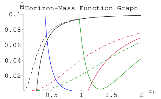
Figure 3: Mass function, $\hat{M}$, versus horizon radius, $r_{h}$: the solid lines represent behavior of the mass function, $\hat{M}$, in noncommutative space for different sets of parameters given in Table 2. The dashed lines represent its behavior in commutative space for the same sets of parameters.

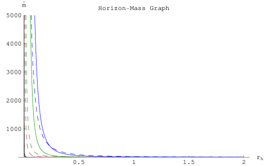
Figure 4: Black hole mass $\hat{m}$ versus horizon radius $r_{h}$: the solid lines represent behavior of the black hole mass $\hat{m}$ in noncommutative space while the dashed lines represent its behavior in commutative space.

In Fig. 3, the solid curves give the representation of the mass function $\hat{M}(r_{h})$ in noncommutative space. The black curve shows asymptotic and increasing behavior whereas blue and red represent decreasing and increasing behavior, respectively, while green shows both of them. The dashed lines correspond to the mass function, $M(r_{h})$, in commutative space. Here, the blue curve represents zero mass function while the remaining curves show increasing behavior. Curves in commutative space extrapolate the mass function.

Figure 4 presents the graphical behavior of the black hole mass. This shows that black, blue and green curves have the same behavior in both commutative and noncommutative spaces. These curves show asymptotic and decreasing behavior while the red curve shows similar behavior in both spaces. It is noteworthy that, for commutative space, the black hole mass always exhibits asymptotic behavior in the region where $m>0$. Noncommutative coordinates show the extrapolation for the black hole mass.

The usual Bardeen black hole temperature, $T_{H}$, is given by [18]

$$T_{H}={\frac{\hbar\partial_{r}F(r)}{4\pi}}|_{r=r_{h}}=\frac{\hbar mr_{h}(r_{h}^{2}-2e^{2})}{2\pi(r_{h}^{2}+e^{2})^{\frac{5}{2}}}$$ (20)

where $F(r)=[1-(2M/r)]$ and $m=(r^{2}+e^{2})^{3/2}/2r^{2}$. For $\hbar=1$, we obtain the following Hawking temperature in noncommutative space:

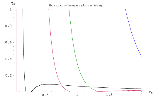
Figure 5: Hawking temperature, $\hat{T}_{H}$, versus horizon radius, $r_{h}$: the solid lines indicate the behavior of temperature, $\hat{T}_{H}$, in noncommutative space while the dashed lines represent its behavior in commutative space.

$$\hat{T}_{H}=\frac{1}{4\pi r_{h}}\left(1+\frac{L_{z}\theta}{4r_{h}^{2}}-\frac{3e^{2}}{r_{h}^{2}}-\frac{5{e^{2}}{L_{z}\theta}}{4r_{h}^{4}}+\frac{2e^{4}}{r_{h}^{4}}+\frac{{e^{4}}{L_{z}\theta}}{2r_{h}^{6}}\right)$$ (21)

It is mentioned here that for large black holes (i.e., $r_{h}^{2}/4\theta\gg 0$) we recover the temperature of the Bardeen regular black hole (20).

Each curve in Fig. 5 shows the behavior of temperature. For noncommutative space, horizon radius and temperature, $\hat{T}_{H}$, of a Bardeen black hole preserve the inverse relation for solid green and blue curves while for the red and black it indicates asymptotic, decreasing, and increasing behavior. For commutative space, dashed green and blue curves indicate that the behavior of temperature, $T_{H}$, does not lie in the region of positive temperature, $T_{H}>0$. However, red and black curves have overlapping behavior with noncommutative space and indicate that $T_{H}\rightarrow 0$ with increasing $r_{h}$. Thus, for all $T_{H}$, commutative coordinates do not show extrapolation for a given set of parameters.

The first law of thermodynamics for a Bardeen regular black hole is

$$dm=TdS+\phi de$$ (22)

where the electric potential of the black hole is given by

$$\phi=\frac{\partial m}{\partial e}|_{r=r_{h}}=\frac{3e}{2r_{h}^{2}}(r_{h}^{2}+e^{2})^{\frac{1}{2}}$$ (23)

The entropy of the black hole is [18]

$$S={\int_{r_{0}}^{r_{h}}}\frac{1}{T_{H}}dm=2\pi\hbar^{-1}\left((-\frac{e^{2}}{r_{h}}+\frac{r_{h}}{2})\sqrt{e^{2}+r_{h}^{2}}+\frac{3}{2}{e^{2}}\ln(r_{h}+\sqrt{e^{2}+r_{h}^{2}})\right)$$ (24)

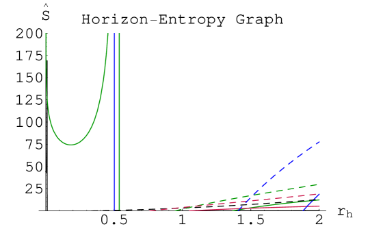
Figure 6: Entropy, $\hat{S}$, versus horizon radius, $r_{h}$: the solid lines represent entropy, $\hat{S}$, of the black hole in noncommutative space while the dashed lines represent the entropy, $S$, of the black hole in commutative space.

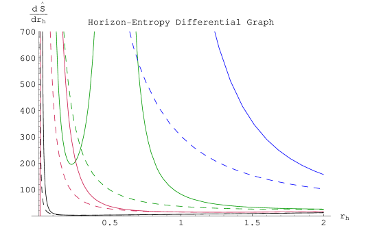
Figure 7: Derivative of entropy with respect to horizon radius, $\frac{d\hat{S}}{dr_{h}}$, versus horizon radius, $r_{h}$: the solid lines show the behavior of $\frac{d\hat{S}}{dr_{h}}$ in noncommutative space while the dashed lines show it in commutative space.

In noncommutative space, it becomes

$$\hat{S} = 2\pi[r_{h}(-\frac{4{e^{2}}r_{h}}{4r_{h}^{2}-L_{z}\theta}+\frac{r_{h}}{2}-\frac{L_{z}\theta}{8r_{h}})(1+\frac{1}{2r_{h}^{2}}(e^{2}-\frac{L_{z}\theta}{2}))$$ (25)

$$+ \frac{3}{2}e^{2}\ln(r_{h}-\frac{L_{z}\theta}{4r_{h}}+r_{h}(1+\frac{1}{2r_{h}^{2}}(e^{2}-\frac{L_{z}\theta}{2})))]$$

The entropy as a function of $r_{h}$ is represented in Fig. 6. In the large black hole limit, the entropy function corresponds to the Bekenstein-Hawking area law relating entropy and horizon area (i.e., $S=A/4$) for the regular black hole geometry.

The derivative of entropy, $S$, (24) with respect to horizon radius, $r_{h}$, in commutative space can be written as

$$\frac{dS}{dr_{h}} = \frac{2\pi}{\hbar}[(-\frac{e^{2}}{r_{h}}+\frac{r_{h}}{2})\frac{r_{h}}{\sqrt{e^{2}+r_{h}^{2}}}+\sqrt{e^{2}+r_{h}^{2}}(\frac{e^{2}}{r_{h}^{2}}+\frac{1}{2})$$ (26)

$$+ \frac{3e^{2}}{2(r_{h}+\sqrt{e^{2}+r_{h}^{2})}}(1+\frac{r_{h}}{\sqrt{e^{2}+r_{h}^{2}}})]$$

In noncommutative space ($\hbar=1$), it becomes

$$\frac{d\hat{S}}{dr_{h}} = 2\pi[(\frac{-4e^{2}r_{h}}{4r_{h}^{2}-L_{z}\theta}+\frac{r_{h}}{2}-\frac{L_{z}\theta}{8r_{h}})(1-\frac{1}{2r_{h}^{2}}(e^{2}-\frac{L_{z}\theta}{2}))$$ (27)

$$+ (r_{h}+\frac{1}{2r_{h}}(e^{2}-\frac{L_{z}\theta}{2}))(\frac{4e^{2}(L_{z}\theta+4r_{h}^{2})}{(4r_{h}^{2}-L_{z}\theta)^{2}}+\frac{1}{2}+\frac{L_{z}\theta}{8r_{h}^{2}})$$

$$+ \frac{3e^{2}(4r_{h}^{2}+L_{z}\theta-e^{2})}{2r_{h}(4r_{h}^{2}-L_{z}\theta+e^{2})}]$$

In Fig. 6, there are two different behaviors of the entropy, $\hat{S}$, in noncommutative space represented by solid lines. Black and red curves indicate asymptotic and linearly increasing behavior, respectively, while blue and green show both of them. The entropy, $S$, in commutative space is shown by dashed lines, where all four of the curves exhibit linearly increasing behavior while only red and black curves extrapolate black hole entropy.

In Fig. 7, both solid lines in noncommutative space indicate entropy differential $\frac{d\hat{S}}{dr_{h}}$ and the dashed lines in the commutative case represent $\frac{dS}{dr_{h}}$ and both exhibit the same behavior. Green, red and black curves show asymptotic behavior while the blue curve indicates that the entropy differential decreases as horizon radius increases. All four of the curves in commutative space extrapolate entropy differential.

The horizon area, $A$, of the Bardeen regular black hole is given by [13]

$$A=r^{2}_{h}{\int^{2\pi}_{0}}d\phi{\int^{\pi}_{0}}\sin\theta d\theta=4\pi{r^{2}_{h}}=16\pi M^{2}=\frac{16\pi{m^{2}}{r_{h}^{6}}}{(r_{h}^{2}+e^{2})^{3}}$$ (28)

For $\hbar=1$, this turns out to be the area in noncommutative space

$$\hat{A}=\frac{16\pi m^{2}(r_{h}^{6}-\frac{3}{2}r_{h}^{4}L_{z}\theta)}{(r_{h}^{6}-\frac{3}{2}L_{z}\theta r_{h}^{4}+3e^{2}r_{h}^{4})}$$ (29)

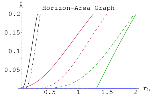
Figure 8: Horizon area, $\hat{A}$, versus horizon radius, $r_{h}$: the solid lines show the area, $\hat{A}$, of the regular black hole in noncommutative space while the dashed lines show the area $A$ in commutative space.

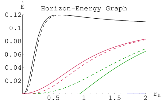
Figure 9: Energy distribution function, $\hat{E}$, versus horizon radius, $r_{h}$: the solid lines represent the energy distribution function, $\hat{E}$, in noncommutative space while the dashed lines represent it in commutative space.

In Fig. 8, the solid lines demonstrate that the area, $\hat{A}$, is zero, corresponding to the blue curve in noncommutative space. The remaining three curves representing area increase linearly with an increase in horizon radius. For commutative space, the dashed lines display the same behavior of area, $A$, as the noncommutative case. For commutative space, horizon area must be positive and extrapolates for the given choice of parameters.

In the Landau-Lifshitz prescription, the energy distribution is [19]

$$E=-\frac{mr_{h}^{3}}{-(r_{h}^{2}+e^{2})^{\frac{3}{2}}+2mr_{h}^{2}}$$ (30)

At large distances or for $e=0$, this reduces to the energy of the Schwarzschild black hole [20]. In noncommutative space, it becomes

$$\hat{E}=-\frac{m(r_{h}-\frac{3L_{z}\theta}{4r_{h}})}{r_{h}(1+\frac{3}{2r_{h}^{2}}(e^{2}-\frac{L_{z}\theta}{2}))+2m(1-\frac{L_{z}\theta}{2r_{h}^{2}})}$$ (31)

In Fig. 9, curves describe the same behavior as that for the corresponding area graph for both noncommutative and commutative spaces. The energy distribution function, $E$, of the regular black hole in commutative space is always positive. Blue and Green curves extrapolate energy in commutative space while black and red have the same behavior in both spaces.

4 Summary

This paper deals with the effects of noncommutative space on the behavior of singularity, horizon, and thermodynamical quantities of Bardeen regular black holes. It also extends our recent work on the thermodynamics of the usual Bardeen black hole [18]. For a suitable choice of parameters, singularity, horizon, mass function, black hole mass, temperature, entropy and its differential, area and energy distribution have been investigated and compared graphically in both commutative and noncommutative spaces.

It has been found that, for horizon radius $r_{h}>0$, there is a class of parameters for which function of horizon radius, $f(r_{h})$, approaches infinity, which leads to a singularity. If the noncommutative parameter $\theta$ approaches zero, then for $r_{h}=0$, $f(r_{h})$ does not approach infinity, which leads to the usual black hole solution without having the essential singularity. For noncommutative space, the Bardeen solution represents the horizon, while the Bardeen solution in commutative space does not represent the horizon for the same sets of parameters.

The behavior of the thermodynamical quantities can be summarized as follows:

• Different curves of the mass function in noncommutative space show decreasing, increasing, and asymptotic behavior while the mass function has increasing behavior for $M>0$ in the commutative case.

• The black hole mass indicates asymptotic behavior for $m>0$ in commutative geometry, while for the noncommutative case, some curves exhibit asymptotic while some represent similar behavior to the commutative case.

• For the noncommutative case, temperature expresses asymptotic, decreasing, and increasing behaviors. For the commutative case, two curves have overlapping behavior with the noncommutative case while temperature approaches zero and as horizon radius increases. The remaining two curves do not show any behavior in the region where $T_{H}\geq 0$ but have asymptotic behavior in the region where $T_{H}<0$.

• The entropy has overlapping behavior (asymptotic and increasing) in the noncommutative case, while it has only increasing behavior in the commutative case. The entropy differential exhibits the same behavior in both spaces.

• Energy and area exhibit the same behavior in both spaces.

• Commutative coordinates extrapolate distances and thermodynamic quantities (except temperature) for a particular choice of parameters.

It would be interesting to extend this analysis to examine the behavior of thermodynamic quantities in noncommutative space for the stringy charged black hole solutions and also for the regular black hole solution with cosmological constant.

Acknowledgment

We would like to thank the Higher Education Commission, Islamabad, Pakistan, for its financial support through the Indigenous Ph.D. 5000 Fellowship Program Batch-IV.

References

- [1] R.J. Szabo. Gen. Relativ. Gravit. 42, 1 (2010).
- [2] R.J. Szabo. Phys. Rep. 378, 207 (2003).
- [3] J. Gomis and T. Mehen. Nucl. Phys. B, 591, 265 (2000).
- [4] S.A. Alavi. Acta Phys. Pol. B, 40, 2679 (2009).
- [5] Y.S. Myung and M. Yoon. Eur. Phys. J. C, 62, 405 (2009).
- [6] J.M. Tejeiro and A. Larranaga. gr-qc/1004.1120v1 (2010).
- [7] P. Nicolini, A. Smailagic and E. Spallucci. Phys. Lett. B, 632, 547 (2006).
- [8] K. Nozari and B. Fazlpour. Mod. Phys. Lett. A, 22, 2917 (2007).
- [9] K. Nozari and B. Fazlpour. Acta Phys. Pol. B, 39, 1363 (2008).
- [10] K. Nozari and S.H. Mehdipour. Commun. Theor. Phys. 53, 503 (2010).
- [11] S. Ansoldi, P. Nicolini, A. Smailagic and E. Spallucci. Phys. Lett. B, 645, 261 (2007).
- [12] E. Spallucci, A. Smailagic and P. Nicolini. Phys. Lett. B, 670, 449 (2009).
- [13] F. Nasseri. Gen. Relativ. Gravit. 37, 2223 (2005).
- [14] J. Sadeghi. Chaos Solitons Fractals, 38, 986 (2008).
- [15] J. Sadeghi and M.R. Setare. Int. J. Theor. Phys. 46, 817 (2007).
- [16] J. Bardeen. In Proceedings of the 5th International Conference on Gravitation and the Theory of Relativity. Tbilisi, Georgia. 9-13 September 1968. Tbilisi Unversty Press, Tbilisi. 1968.
- [17] L. Kang and D. Sayipjamal. Chin. Phys. C, 34, 944 (2010).
- [18] M. Sharif and W. Javed. J. Korean Phys. Soc. 57, 217 (2010).
- [19] I. Radinschi and B. Ciobanu. Rom. Journ. Phys. 50, 1223 (2005).
- [20] M. Sharif. Nuovo Cimento Soc. Ital. Fis., B, 119, 463 (2004).