The creation of radiation and the relic of inflaton potential

Abstract

Recently, we have performed research on the subject of the cosmological constant problem. The scenario is based on two postulates for inflationary theory: one is that inflaton $\phi$ can interact with radiation (relativistic particles); the other is that radiation will be created continuously during and after the epoch of inflation. According to these postulates and from a “macroscopic perspective”, we discover that radiation can be viewed as a product of the interaction between $\dot{\phi}$ and some “effective kinetic frictional force” that exists in inflaton dynamics. Deducing and surmising from “effective friction”, we obtain conclusions of two special types of expanding universe: A Type I universe will finally enter an expanding course after a special time $t_{*}$ with uniformly rolling $\dot{\phi}\left(t_{*}\right)$ due to the balance between $V^{{}^{\prime}}\left(\phi\left(t\right)\right)$, $3H\left(t\right)\dot{\phi}\left(t_{*}\right)$ and the “effective kinetic frictional force”. In this result, the expanding course will see particles created continuously. Additionally, for a Type II universe, $\phi$ will be at rest after $t_{r}$ inside a region named the “stagnant zone” that is formed by the “maximum effective static frictional force”. Consistent with this, inflaton potential will survive as a relic $V\left(\phi\left(t_{r}\right)\right)$, playing the role of the effective cosmological constant $\Lambda$.

1 Introduction

According to the research and observations of Friedman [1], Lemaître [2] and Hubble [3], Einstein and other physicists have been told that it is not necessary to insert a cosmological term $\lambda$ into the general theory of relativity. Therefore, until 1998 most believed that the expansion of our universe is — or will be — slowing down. Nevertheless, much observational data from [5, 6, 7, 8, 9, 10, 11] provides evidence to oppose intuition: our universe is presently expanding with acceleration. Besides, [12, 13, 14, 15, 16, 17, 18, 19, 20, 21, 22] have been/are being performed to excavate greater understandings: we now know that the major components required to build the current universe are roughly 0.008% radiation, 5% observable matter and 22% dark matter. In particular, the surplus energy density that we call dark energy confirms that a new discovery, i.e. accelerating expansion, is needed.

Obviously, the part of dark energy is a compelling mystery because few of its properties are known. Those which we do have knowledge of are as follows: to begin, the first Friedman equation without the cosmological term,

$$\frac{\ddot{\mathbb{R}}\left(t\right)}{\mathbb{R}\left(t\right)}=-\frac{\kappa c^{2}}{6}\left(\varepsilon+3p\right),$$ (1.1)

shows that the equation of state for dark energy $w_{\mathrm{DE}}\equiv\nicefrac{{p}}{{\varepsilon}}<-\nicefrac{{1}}{{3}}$ (where $c$ is the speed of light; $\varepsilon$ is the dark energy density; $p$ is the pressure of dark energy; $\mathbb{R}\left(t\right)$ is the spatial scale factor; and $t$ is cosmic time) should be satisfied in order to make the “anti-gravity”, $\ddot{\mathbb{R}}=\frac{d^{2}\mathbb{R}}{dt^{2}}>0$, become possible on the large scales of our universe; secondly, the repulsive property of dark energy requires its distribution to be highly homogeneous and isotropic; and finally there is still no evidence to suggest that dark energy interacts with matter through any of the fundamental forces other than gravity. In order to explain/illustrate this impalpable phenomenon, many models [24, 25, 26, 27, 28, 29, 30, 31, 32, 33, 34, 35, 36, 37, 38, 39, 40, 41, 42, 43, 44] have been proposed. Of course, observations also lead to a rethink of the cosmological term that was thrown in Einstein’s trashcan. Picking up the term is excellent and simple for analyzing the new discovery. Consequently, however, a question cannot be avoided: What, practically, is the cosmological term/constant?

To answer, it was thought by [45] that the vacuum energy density discovered in research on quantum field theory might be the cosmological constant. Therefore, the Planck vacuum energy density (PVED) could be calculated by summing the zero-point energies of all normal modes $k$ of some field of mass $m$ up to a wave cut-off, $k_{\mathrm{cut}}=\sqrt{\pi^{2}c^{3}\left(\hbar G\right)^{-1}}\gg mc\hbar^{-1}$, as

$$\left\langle\varepsilon_{\mathrm{Planck}}\right\rangle_{\mathrm{vac}}=\frac{\hbar}{2\left(2\pi\right)^{3}}\int_{0}^{k_{\mathrm{cut}}}4\pi k^{2}dk\sqrt{k^{2}c^{2}+m^{2}c^{4}\hbar^{-2}}\simeq 5.6\times 10^{126}\,\nicefrac{\mathrm{eV}}{\mathrm{cm^{3}}}$$ (1.2)

This is provided by the assumption that the smallest limit of general relativity is the Planck scale. Correspondingly, assuming that the cosmological constant $\Lambda$ is, in fact, dark energy, its value is

$$\varepsilon_{\Lambda}\simeq\frac{3H_{\mathrm{now}}^{2}}{\kappa c^{2}}\times 73\%\simeq 3.76\times 10^{3}\,\nicefrac{\mathrm{eV}}{\mathrm{cm^{3}}},$$ (1.3)

which can be shown by the Hubble rate at its present day value of $H_{\mathrm{now}}\approx 70\,\nicefrac{\mathrm{\nicefrac{\mathrm{km}}{\mathrm{s}}}}{\mathrm{Mpc}}$. Unfortunately, the PVED is too massive in comparison with the effective density as witnessed in reality. Other conditions of vacuum energy density, such as spontaneous symmetry breaking (SSB) in electroweak (EW) theory and the vacuum transition of quantum chromodynamics (QCD), are also expelled as candidates for the cosmological constant because we receive even larger values as

$$\begin{array}[]{l}\left\|\left\langle\varepsilon_{\mathrm{EW}}\right\rangle_{\mathrm{SSB}}\right\|\thickapprox 10^{56}\,\nicefrac{\mathrm{eV}}{\mathrm{cm^{3}}},\\ \left\langle\varepsilon_{\mathrm{QCD}}\right\rangle_{\mathrm{vac}}\thickapprox 10^{44}\,\nicefrac{\mathrm{eV}}{\mathrm{cm^{3}}}.\end{array}$$ (1.4)

Two serious problems are yet indicated by [48, 49]: (i) Where are these densities? (ii) Why is the cosmological constant so small?

Even though vacuum energy densities cannot be the cosmological constant, they are still needed for the investigation of the very early universe. Realizing the inexplicable problems which emerge when observations are made using Hot Big Bang theory, Starobinsky, Guth and others devised a beautiful solution: they suggested that our universe must have inflated itself from a very small size — perhaps just a little bigger than a Planck point [62, 63, 64, 65]. Therefore, according to inflationary theory, a vacuum energy density dependent on the initial size of the universe is required to trigger inflation at the beginning. However, a timely mechanism is also needed to cancel out a huge density at the proper stage, and then to help our universe in exiting from inflation. This is because the expansion of a universe cannot dilute or deplete the vacuum energy density. The solution raises new quandaries: What is the mechanism? Will any relic of the vacuum energy density survive under the effect of this mechanism?

From the statement above, one can imagine that people are attracted and puzzled in equal measure by questions about the existence of the cosmological constant and vacuum energy densities. As evidenced by [45, 46, 47, 48, 49, 50, 51, 52, 53, 54, 55, 56, 57, 58, 59, 60] and similar thinking that we have already mentioned, much work has been proposed and undertaken around these questions. Impressively, [45] and several physicists have noted that the cosmological constant can safely and gracefully coexist with general relativity due to the elegant mathematics and the requirements of particle physics theory. A voice [59] was sounded in the spirit of [45] recently: Is it possible to set the cosmological term as a fundamental constant like the speed of light $c$ and the Planck constant $\hbar$? Regrettably, things are not so simple since two coincidental problems cannot be abandoned. First, the second Friedman equation with a “fundamental Einstein’s cosmological term $\lambda$” in flat spacetime can be written as

$$H^{2}=\frac{\kappa c^{2}}{3}\left(\left\langle\varepsilon_{\mathrm{ord}}\right\rangle+\left\langle\varepsilon_{\mathrm{vac}}\right\rangle\right)+\frac{\lambda c^{2}}{3}$$ (1.5)

(where $H=\nicefrac{{\dot{\mathbb{R}}}}{{\mathbb{R}}}$ is the Hubble rate, and the total energy density is $\left\langle\varepsilon_{\mathrm{ord}}\right\rangle+\left\langle\varepsilon_{\mathrm{vac}}\right\rangle$, which can be separated into two parts: the ordinary and the vacuum). This asserts that the “effective cosmological constant (ECC) $\Lambda$” in density formation would be

$$\varepsilon_{\Lambda}=\left\langle\varepsilon_{\mathrm{vac}}\right\rangle+\frac{\lambda}{\kappa}.$$ (1.6)

Indeed, a negative $\lambda$ could cancel the vacuum density out. Nonetheless, the coincidence is too great for it to be identical to the needed value when (1.3) is compared to (1.2) and (1.4), as each of these is dependent on the chosen inflationary theory. There is another coincidence too: that $\lambda$ will appear at a specific cosmic time, thereby fulfilling the condition of inflationary theory that is employed to help our universe in ending inflation (such as $t_{\mathrm{end}}\lesssim 10^{-36}\,\mathrm{s}$ for the inflation that begins when the universe’s size is close to the Planck point). The second problem is particularly curious: the “fundamental constant $\lambda$” is most strange because it did not originally exist and could not have appeared too early or too late, as otherwise our universe would have turned out totally differently to the one we see today.

Surely, if another mechanism without these coincidental problems could be found, keeping the fundamental constant $\Lambda$ as (or close to) (1.3) would be perfectly acceptable.

Luckily, the Klein-Gordon equation edifies with the assertion that scalar field dynamics could perform a process for decaying scalar potential energy by self-interaction. [46] and others employed this concept and introduced the scalar field $\phi$, named inflaton, as the quantum matter in the epoch before the phase transition of Grand Unification Theory (GUT). Followingly, the Friedman equations with only $\phi$ in flat spacetime are

$$\frac{\ddot{\mathbb{R}}}{\mathbb{R}}=-\frac{\kappa}{3}\left(\dot{\phi}^{2}-c^{2}V\left(\phi\right)\right),$$ (1.7)

$$\left(\frac{\dot{\mathbb{R}}}{\mathbb{R}}\right)^{2}=\frac{\kappa}{3}\left(\frac{1}{2}\dot{\phi}^{2}+c^{2}V\left(\phi\right)\right),$$ (1.8)

where $\phi=\phi\left(t\right)$ is only dependent on time and $V\left(\phi\right)$ is the inflaton potential with a minimum value of zero. Clearly, $t_{i}$ sets the start time for inflation; $V\left(\phi\left(t_{i}\right)\right)$ is the vacuum energy density that triggers the inflation of the universe. On the other hand, $V\left(\phi\left(t_{r}\right)\right)$ can be treated as a cosmological constant when $\phi$ comes to rest at $t\geqslant t_{r}$. To derive (1.8) with respect to $t$, the field equation in dynamic spacetime can be found as

$$-3H\dot{\phi}^{2}=\frac{d}{dt}\left(\frac{1}{2}\dot{\phi}^{2}+c^{2}V\left(\phi\right)\right).$$ (1.9)

Equation (1.9) tells us that the damping term $3H\dot{\phi}^{2}$ will consume energy from $V\left(\phi\left(t_{i}\right)\right)$ when a universe is expanding. Evidently, $V\left(\phi\left(t_{r}\right)\right)$ is zero since the total energy of $\dot{\phi}^{2}$ and $V\left(\phi\right)$ will be used up in the end. In this scenario, it looks as if setting a nonzero minimum of $V\left(\phi\right)$, or allowing the insertion of “$\Lambda$” into (1.7) and (1.8) are the only methods for obtaining the cosmological constant.

Well, if one still believes that the cosmological constant is a “product” of the evolution of the universe, what can one do to search for this mechanism? Actually, the scenario presented in (1.7) and (1.8) is too simple because it only includes quantum matter. Such limitations lead to another question: Is it possible that the process of creating matter in the early universe could hint towards the building mechanism for the cosmological constant? Following the above conjecture and the fact that (1.9) is an oscillating equation, there is a simple but useful example that arises in daily life: a spring oscillating system on the rough surface of a table, as in Figure 1 .

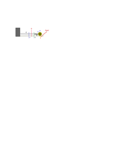
Figure 1: A spring oscillating system is placed on a rough table: $\mathrm{k}$ is the spring constant; $\boldsymbol{\mathbf{F}}$ is the restoring force of the spring; $\boldsymbol{\mathbf{f}}$ is the frictional force between the oscillator and the table-surface; the mass of the oscillator is $M$; “$0$” is the position of the spring’s original length; and $\left[x_{-},x_{+}\right]$ is the stagnant zone of the oscillator.

If the amount of kinetic frictional force is set equal to the maximum static frictional force, the equations of motion will be

$$M\ddot{x}+\mathrm{k}x=+f,\quad\mathrm{for}\>\dot{x}<0,$$ (1.10)

$$M\ddot{x}+\mathrm{k}x=-f,\quad\mathrm{for}\>\dot{x}>0.$$ (1.11)

$t$ denotes the time of lab frame and $f$ is the amount of frictional force between the table-surface and the oscillator, $M$. (1.10) can now be rewritten as a phase equation with the moment $\boldsymbol{\mathbf{P}}$ and position $\boldsymbol{\mathbf{x}}$:

$$\frac{P^{2}\left(t\right)}{M\mathrm{k}\left(x\left(n\mathrm{T}\right)-\frac{f}{\mathrm{k}}\right)^{2}}+\frac{\left(x\left(t\right)-\frac{f}{\mathrm{k}}\right)^{2}}{\left(x\left(n\mathrm{T}\right)-\frac{f}{\mathrm{k}}\right)^{2}}=1,$$ (1.12)

$\mathrm{T}=2\pi\sqrt{\frac{M}{\mathrm{k}}}$ is the period of oscillation. This equation only applies to the interval of time $n\mathrm{T}\leq t\leq\frac{2n+1}{2}\mathrm{T}$, where $n=0,1,2,\cdots$. In addition, (1.11) becomes

$$\frac{P^{2}\left(t\right)}{M\mathrm{k}\left(x\left(\frac{2n+1}{2}\mathrm{T}\right)+\frac{f}{\mathrm{k}}\right)^{2}}+\frac{\left(x\left(t\right)+\frac{f}{\mathrm{k}}\right)^{2}}{\left(x\left(\frac{2n+1}{2}\mathrm{T}\right)+\frac{f}{\mathrm{k}}\right)^{2}}=1,$$ (1.13)

which is available during $\frac{2n+1}{2}\mathrm{T}\leq t\leq\left(n+1\right)\mathrm{T}$, where $n=0,1,2,\cdots$. Figure 2

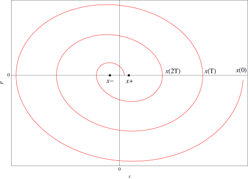
Figure 2: This is the phase diagram cited in the example. According to (1.12), $x_{+}$ is the center of the elliptical path of the bottom part; $x_{-}$ is the other center of the upper part, obtained from (1.13). It is clear that the oscillator will stop forever at the position inside the stagnant zone when its amplitude is not bigger than $\left\|x_{\pm}-0\right\|$.

and the stagnant zone, $\left[x_{+}=\frac{+f}{\mathrm{k}},x_{-}=\frac{-f}{\mathrm{k}}\right]$, can be drawn through (1.12) and (1.13).

We will see that the nonzero oscillator’s potential might survive if the oscillator itself rests at a position that is not the origin inside the stagnant zone.

We can now assume certain kinds of “effective friction” and introduce them to (1.9). Moreover, the part of radiation that should be inserted into (1.7) and (1.8) comes as the result of the work done by “effective kinetic frictional force”. This is similar to the above example, and it will hopefully help us to obtain the “stagnant zone” of $\phi$ and then to find the final range of the remaining potential $V\left(\phi\left(t_{r}\right)\right)$.

Inspired by the example of the spring oscillating system, we will now develop our idea in order to build the cosmological constant. The following paper is organized in this way: Firstly, we will illustrate the energy relation between inflaton $\phi$ and radiation (relativistic particles) in a homogeneous and isotropic universe. Next, according to the settings of Section 2, we will introduce two fundamental postulates to build the theory of thermo-inflation. In Section 4, from the order of radiation creation discussed in Section 2, we deduce that “effective frictional force” can exist in inflaton dynamics, and use this result to help discover the relic of inflaton potential. Then, by considering the conditions of “effective friction”, two special types of universe will be shown: a Type I universe will finally enter an expanding course with uniformly rolling $\dot{\phi}\left(t_{*}\right)$ after $t_{*}$, and particles will be created continuously during this course; in a Type II universe, a relic of inflaton potential, $V\left(\phi\left(t_{r}\right)\right)$, will survive to become the ECC $\Lambda$ when $\phi$ is at rest after $t_{r}$. Conclusions will be provided in Section 5.

It should be noted that, in the following sections, we use the Planck units: $c=G=k_{\mathrm{B}}=\hbar=1$. Unless specifically mentioned, $t$, $\tau$ and $\eta$ are employed as the cosmic time, and $t_{i}$ denotes the point at which inflation was beginning and $\phi$ comes to rest at $t\geqslant t_{r}$.

2 The energy relation between inflaton and radiation

2.1 Models

First of all, the energy-momentum tensors of the material in the universe must be recorded. Since the epoch that interests us is earlier than GUT phase transition, most of the material at this time can be considered as a quantum matter, inflaton $\phi\left(x^{\mu}\right)$, which is a kind of scalar field. In our scenario, $\phi$ is real and its energy-momentum tensor is

$$T_{\mu\nu}^{\left(\phi\right)}=\partial_{\mu}\phi\partial_{\nu}\phi-g_{\mu\nu}\left[\frac{1}{2}g^{\alpha\beta}\partial_{\alpha}\phi\partial_{\beta}\phi-V\left(\phi\right)\right],$$ (2.1)

where $V\left(\phi\right)$ is the inflaton potential. In addition, assuming that radiation can simultaneously exist, its energy-momentum tensor should be

$$T_{\mu\nu}^{\left(\mathrm{r}\right)}=\frac{\varepsilon_{\mathrm{r}}\left(t\right)}{3}\left(4u_{\mu}u_{\nu}-g_{\mu\nu}\right)$$ (2.2)

owing to the pressure of radiation $p_{\mathrm{r}}=\nicefrac{{\varepsilon_{\mathrm{r}}}}{{3}}$ (where $u_{\mu}$ is the 4-velocity and $\varepsilon_{\mathrm{r}}$ is the energy density of radiation).

Once this is complete, the distribution of inflaton and radiation in spacetime, and the spacetime geometry of the very early universe are also required. Considering our goal is to search for the mechanism that builds the cosmological constant, the equation of general relativity without the cosmological term should be used, as

$$R_{\mu\nu}-\frac{1}{2}Rg_{\mu\nu}=-16\pi\underset{j}{\sum}T_{\mu\nu}^{\left(j\right)},$$ (2.3)

where $R$ is the Ricci scalar, and $\underset{j}{\sum}T_{\mu\nu}^{\left(j\right)}$ is the total energy-momentum tensor. According to observations, our universe is homogeneous and isotropic on large scales, meaning that the left hand side of the equal sign in (2.3) should be very close to the off-diagonal. For the sake of simplicity, each individual component of $T_{\mu\nu}^{\left(j\right)}$ is undoubtedly off-diagonal as well. Therefore, the distribution of radiation in flat spacetime is

$$\left[u_{\mu}\right]=\left(1,0,0,0\right),$$ (2.4)

in which the mean velocity of radiation in an arbitrary spatial direction is $u_{k}=0$ to satisfy the requirement of there being no net current of matter in the universe. Furthermore, setting $\phi\left(x^{\mu}\right)=\phi\left(t\right)$ to guarantee that $T_{\mu\nu}^{\left(\phi\right)}$ will not violate actual observations of our universe, the components of $T_{\mu\nu}^{\left(\phi\right)}$ are

$$\begin{array}[]{l}T_{00}^{\left(\phi\right)}=\varepsilon_{\phi}\left(t\right)=\frac{1}{2}\dot{\phi}^{2}+V,\\ T_{kk}^{\left(\phi\right)}=p_{\phi}\left(t\right)=\frac{1}{2}\dot{\phi}^{2}-V,\\ T_{kl}^{\left(\phi\right)}=0,\;\left(k\neq l\right).\end{array}$$ (2.5)

Finally, we assume that the initial universe is flat, as consistent with our previous discussion. It means that the FRW line element should be

$$ds^{2}=dt^{2}-\mathbb{R}^{2}\left(t\right)\left(dx^{2}+dy^{2}+dz^{2}\right),$$ (2.6)

as the background of the universe’s spacetime.

2.2 Energy conservation and interaction

Noether taught us that an isolated physical system should obey the requirement of its total action being invariant under an infinitesimal coordinate transformation. This leads to a conservation law of

$$D_{\mu}\left(\underset{j}{\sum}T_{\left(j\right)}^{\mu\nu}\right)=0$$ (2.7)

in curved spacetime, where $D_{\mu}$ is the covariant derivative and $\sum_{j}$ means a system with several matter fields. By this reasoning, if we assume that our universe is unique or adiabatic, as per the discussion in the previous subsection, $D_{\mu}\left(T_{\left(\mathrm{r}\right)}^{\mu\nu}+T_{\left(\phi\right)}^{\mu\nu}\right)=0$ must be satisfied. For $\nu=0$, the energy conservation is obeyed by

$$\dot{\varepsilon}_{\mathrm{r}}+4H\varepsilon_{\mathrm{r}}=-\left(\dot{\varepsilon}_{\phi}+3H\dot{\phi}^{2}\right),$$ (2.8)

which clearly shows the relationship of energy transference between $\phi$ and radiation. Thus we further consider the situation of interaction, and (2.8) can be separated into two situations:

Situation 1:

There is no interaction between $\phi$ and radiation. This is popular for discussion purposes. In this situation, (2.8) obeys

$$\dot{\varepsilon}_{\mathrm{r}}+4H\varepsilon_{\mathrm{r}}=0,\quad\dot{\varepsilon}_{\phi}+3H\dot{\phi}^{2}=0.$$ (2.9)

Obviously, the components of both radiation and $\phi$ are closed, since energy cannot transfer between the two.

Situation 2:

Some interaction exists between $\phi$ and radiation. A similar property is first considered for the case of quintessence and matter by Zimdahl et al. [41]. In this situation, the interaction term $Q\left(t\right)$ can be introduced into (2.8) as

$$\dot{\varepsilon}_{\mathrm{r}}+4H\varepsilon_{\mathrm{r}}=Q\left(t\right),\quad\dot{\varepsilon}_{\phi}+3H\dot{\phi}^{2}=-Q\left(t\right).$$ (2.10)

It follows that $\phi$ and radiation are open to each other.

3 Theory of thermo-inflation

3.1 Postulates

The properties for creating radiation before and after GUT phase transition must be outlined. We suggest following postulates for our scenario:

Postulate A:

There exists some interaction between $\phi$ and radiation.

Postulate B:

Radiation can be created continuously during and after the epoch of inflation. [67, 68]

Alternatively, when considering the creation of radiation in an adiabatic universe, Prigogine et al. [66] suggest the thermal condition of an open system of radiation

$$d\left(\varepsilon_{\mathrm{r}}v\right)+p_{\mathrm{r}}dv-\frac{h_{\mathrm{r}}}{n_{\mathrm{r}}}d\left(n_{\mathrm{r}}v\right)=0,$$ (3.1)

which obeys the first law of thermodynamics ($h_{\mathrm{r}}=\varepsilon_{\mathrm{r}}+p_{\mathrm{r}}=\frac{4}{3}\varepsilon_{\mathrm{r}}$; $v\propto\mathbb{R}^{3}$ is the comoving volume of the universe; $n_{\mathrm{r}}\left(t\right)=\nicefrac{{N_{\mathrm{r}}\left(t\right)}}{{v\left(t\right)}}$ is the number density of relativistic particles; and $N_{\mathrm{r}}\left(t\right)$ is the number of particles in the whole universe). (3.1) has another easily calculable form as

$$\dot{\varepsilon}_{\mathrm{r}}+4H\varepsilon_{\mathrm{r}}=\frac{4}{3}\Gamma\varepsilon_{\mathrm{r}},$$ (3.2)

where $\Gamma\left(t\right)\equiv\nicefrac{{\dot{N}_{\mathrm{r}}}}{{N_{\mathrm{r}}}}$ is the particle creation rate. The solution of radiation energy density $\varepsilon_{\mathrm{r}}$ is

$$\varepsilon_{\mathrm{r}}\left(t\right)=\varepsilon_{\mathrm{r}}\left(t_{a}\right)\exp\left(\frac{4}{3}\int_{t_{a}}^{t}\left(\Gamma-3H\right)d\tau\right),$$ (3.3)

where $t_{a}$ is an arbitrary cosmic time for the commencement of observation. Besides, comparing (3.2) with (2.8), $\Gamma$ could be described as

$$\Gamma=-\frac{\dot{\varepsilon}_{\phi}+3H\dot{\phi}^{2}}{\frac{4}{3}\varepsilon_{\mathrm{r}}}.$$ (3.6)

Because of Postulate B, the value of $\Gamma$ should NOT be less than zero. It leads to the fact that $\dot{\varepsilon}_{\phi}+3H\dot{\phi}^{2}\leq 0$ (the interaction term $Q\left(t\right)=\frac{4}{3}\Gamma\varepsilon_{\mathrm{r}}\geq 0$) happens in an expanding universe. Therefore, in our scenario, the energy of $\phi$ will decrease with time and flow into radiation creation. In other words, the discovery of (3.2) gives us an important and specific message: if we believe that our universe was created from a vacuum, the energy relationship between quantum matter and real matter should satisfy Situation 2.

Introducing (2.5) into (3.6), we easily find that radiation is created by the moving $\phi$. Moreover, the following equation is relevant,

$$\underset{\dot{\phi}\rightarrow 0}{\lim}\Gamma\left(t\right)=-\underset{\dot{\phi}\rightarrow 0}{\lim}\frac{\left(\ddot{\phi}+V^{{}^{\prime}}\left(\phi\right)+3H\dot{\phi}\right)\dot{\phi}}{\frac{4}{3}\varepsilon_{\mathrm{r}}}=0,$$ (3.7)

where $V^{{}^{\prime}}\left(\phi\right)=\frac{dV}{d\phi}$. Consequently there is no radiation created when the “instantaneous speed” of $\phi$ is zero. Of course, radiation will no longer be created when $t\geq t_{r}$.

3.2 Field equations and solutions

Relying on (2.3), the Friedman equations with field $\phi$ and radiation can be written as

$$\frac{\ddot{\mathbb{R}}}{\mathbb{R}}=-\frac{8\pi}{3}\left(\dot{\phi}^{2}-V\left(\phi\right)+\varepsilon_{\mathrm{r}}\right),$$ (3.8)

$$\left(\frac{\dot{\mathbb{R}}}{\mathbb{R}}\right)^{2}=\frac{8\pi}{3}\left(\frac{1}{2}\dot{\phi}^{2}+V\left(\phi\right)+\varepsilon_{\mathrm{r}}\right).$$ (3.9)

The employment of the relationship $p_{\mathrm{r}}=\nicefrac{{\varepsilon_{\mathrm{r}}}}{{3}}$ is again worthy of attention. To derive both sides of the equal sign in (3.9) with respect to $t$, and to combine our result with (3.8), we have

$$-H\left(3\dot{\phi}^{2}+4\varepsilon_{\mathrm{r}}\right)=\frac{d}{dt}\left(\frac{1}{2}\dot{\phi}^{2}+V+\varepsilon_{\mathrm{r}}\right)=\frac{3}{4\pi}H\dot{H}.$$ (3.10)

It gives the solution of the Hubble rate

$$H\left(t\right)=H\left(t_{i}\right)-\frac{4\pi}{3}\int_{t_{i}}^{t}\left(3\dot{\phi}^{2}+4\varepsilon_{\mathrm{r}}\right)d\tau,$$ (3.11)

and therefore the spatial scale factor is

$$\mathbb{R}\left(t\right)=\mathbb{R}\left(t_{i}\right)\exp\left[\int_{t_{i}}^{t}\left(H\left(t_{i}\right)-\frac{4\pi}{3}\int_{t_{i}}^{\eta}\left(3\dot{\phi}^{2}+4\varepsilon_{\mathrm{r}}\right)d\tau\right)d\eta\right].$$ (3.12)

(3.10) also provides the evolution of radiation density:

$$\varepsilon_{\mathrm{r}}\left(t\right)=-\frac{3}{16\pi}\dot{H}-\frac{3}{4}\dot{\phi}^{2}.$$ (3.13)

This is the other form of (3.3). Next, comparing (3.8) with the second derivative of (3.12) (with respect to $t$), a solution for the inflaton potential becomes clear:

$$V\left(t\right)=\frac{3}{8\pi}\left[H\left(t_{i}\right)-\frac{4\pi}{3}\int_{t_{i}}^{t}\left(3\dot{\phi}^{2}+4\varepsilon_{\mathrm{r}}\right)d\tau\right]^{2}-\frac{1}{2}\dot{\phi}^{2}\left(t\right)-\varepsilon_{\mathrm{r}}\left(t\right),$$ (3.14)

or

$$V\left(t\right)=\frac{1}{4}\dot{\phi}^{2}+\frac{R}{32\pi},$$ (3.15)

where $R=6\dot{H}+12H^{2}$ is the Ricci curvature. Attention should be drawn to the fact that $V\left(t\right)$ is the expansion in $t$ of $V\left(\phi\left(t\right)\right)$; it is not $V\left(\phi,t\right)$.

4 “Effective friction” and the relic of inflaton potential

4.1 Definition of the effective friction

In this section, our mission is to demonstrate that an effect similar to friction could exist in inflaton dynamics. Suppose that the inflaton is affected by the effect, its equation of motion will be

$$\ddot{\phi}+3H\dot{\phi}+V^{{}^{\prime}}\left(\phi\right)=\pm f_{\phi k},$$ (4.1)

where the source term $f_{\phi k}$ is the “effect/force” that we assume and wish to find out. In addition, the direction of the force is defined by “$+$” or “$-$”. The “$+$” direction follows the situation of $\dot{\phi}<0$; “$-$” will be adopted if $\dot{\phi}>0$.

Next, in order to obtain the equation as (4.1), we introduce (3.2) into the calculating result of (3.10). We obtain

$$\dot{\phi}\ddot{\phi}+3H\dot{\phi}^{2}+V^{{}^{\prime}}\left(\phi\right)\dot{\phi}=-\frac{4}{3}\Gamma\varepsilon_{\mathrm{r}}.$$ (4.2)

According to the discussion of (3.6), the negative sign of (4.2) shows that energy is transferred from $\phi$ to radiation. Taking the macroscopic viewpoint, and comparing (4.2) with (1.10) and (1.11), $-\frac{4}{3}\Gamma\varepsilon_{\mathrm{r}}$ can be regarded as the power resulting from some “kinetic frictional force”, just like the example in Section 1. Rewriting (4.2) as

$$\ddot{\phi}+3H\dot{\phi}+V^{{}^{\prime}}\left(\phi\right)=-\frac{4\Gamma\varepsilon_{\mathrm{r}}}{3\dot{\phi}},$$ (4.3)

we have the following conclusion after comparing (4.3) with (4.1):

$$\mathbf{f}_{\phi k}\equiv-\frac{4\Gamma\varepsilon_{\mathrm{r}}}{3\dot{\phi}}.$$ (4.4)

Here $\mathbf{f}_{\phi k}$ is the vector-form of $f_{\phi k}$, and its direction is indeed opposite to the direction of $\dot{\phi}$ due to the conclusion of the positive interaction term $Q\left(t\right)$ from (2.10) and (3.6). Therefore, $\mathbf{f}_{\phi k}$ can be defined as the “Effective Kinetic Frictional Force” (EKFF) of the oscillating system of $\phi$ ($\phi$-system for short). Furthermore, (4.3) provides the additional information of the “Effective Static Frictional Force” (ESFF), as

$$\left\|\boldsymbol{\mathbf{f}}_{\phi s}\right\|=\underset{\dot{\phi}\rightarrow 0}{\lim}\left\|-\frac{4\Gamma\varepsilon_{\mathrm{r}}}{3\dot{\phi}}\right\|.$$ (4.5)

At first glance, $\left\|\boldsymbol{\mathbf{f}}_{\phi s}\right\|$ seems to cause confusion because it looks like divergent. In actual fact, this is not a matter for worry because a static frictional force does zero work. This means that a finite $\left\|\boldsymbol{\mathbf{f}}_{\phi s}\right\|$ can exist in the $\phi$-system as per the discussion of (3.7).

4.2 Two special types of universe

To apply the conclusion of “effective friction”, the universe can be roughly sorted by two special conditions of (4.3) and (4.5). These conditions and the corresponding universe types are:

1. Type I universe — expanding with an uniform $\dot{\phi}\left(t_{*}\right)$: For a variable EKFF, it and the damping term $-3H\left(t\right)\dot{\phi}\left(t_{*}\right)$ will cancel out the restoring force $-V^{{}^{\prime}}\left(\phi\left(t\right)\right)$ after the special time $t_{*}$, causing $\dot{\phi}$ to become the uniform velocity $\dot{\phi}\left(t_{*}\right)$. In consequence, the universe will enter an expanding mode as

   $$\mathbb{R}\left(t\right)=\mathbb{R}\left(t_{*}\right)\exp\left[-\int_{t_{*}}^{t}\left(\frac{4\Gamma\left(\tau\right)\varepsilon_{\mathrm{r}}\left(\tau\right)}{9\dot{\phi}^{2}\left(t_{*}\right)}+\frac{V^{{}^{\prime}}\left(\phi\left(\tau\right)\right)}{3\dot{\phi}\left(t_{*}\right)}\right)d\tau\right].$$ (4.6)

   Another important property of this type can also be discovered: particles would have had a period of creation after $t_{*}$. The range of the particle creation rate should be

   $$0<\Gamma\left(t\right)<-\frac{3V^{{}^{\prime}}\left(\phi\left(t\right)\right)\dot{\phi}\left(t_{*}\right)}{4\varepsilon_{\mathrm{r}}\left(t\right)},$$ (4.7)

   where $t\geq t_{*}$. However, this will be invalid after the universe enters the next stage (such as $\dot{\phi}$ will not be uniform).

   Example:

   We are drawn to Hoyle’s 1948 model [69] since a Type I universe can create particles continuously even when its age is much older than the epoch of inflation. Now, let us consider a toy condition in which the matter of a special Type I universe is always radiation. The Hubble rate of such a universe can actually be found from (3.13), as

   $$H\left(t\right)=H\left(t_{\ddagger}\right)-\frac{4\pi}{3}\left(3\dot{\phi}^{2}\left(t_{*}\right)+4\varepsilon_{\mathrm{r}}\left(t_{\ddagger}\right)\right)\left(t-t_{\ddagger}\right),$$ (4.8)

   which satisfies the requirement that the matter density of Hoyle’s universe will become static after $t_{\ddagger}$ (the time-relationship is $t\geq t_{\ddagger}\geq t_{*}$). In this case, (4.3) and (4.8) provide an interesting and important result of

   $$3\dot{\phi}\left(t_{*}\right)V^{{}^{\prime}}\left(\phi\left(t\right)\right)+4\varepsilon_{\mathrm{r}}\left(t_{\ddagger}\right)\Gamma\left(t\right)=$$

   $$-9\dot{\phi}^{2}\left(t_{*}\right)H\left(t_{\ddagger}\right)+12\pi\dot{\phi}^{2}\left(t_{*}\right)\left(3\dot{\phi}^{2}\left(t_{*}\right)+4\varepsilon_{\mathrm{r}}\left(t_{\ddagger}\right)\right)\left(t-t_{\ddagger}\right)$$ (4.9)

   since $\ddot{\phi}\left(t\geq t_{*}\right)=0$. In addition, to introduce (4.8) into (3.9) with conditions of $\dot{\phi}\left(t\right)=\dot{\phi}\left(t_{*}\right)$, $\varepsilon_{\mathrm{r}}\left(t\right)=\varepsilon_{\mathrm{r}}\left(t_{\ddagger}\right)$ and $V\left(\phi\right)=V\left(\phi\left(t\right)\right)$, the value of inflaton potential at $t$ can be obtained as

   $$V\left(\phi\left(t\right)\right) = \frac{3}{8\pi}\left[H\left(t_{\ddagger}\right)-\frac{4\pi}{3}\left(3\dot{\phi}^{2}\left(t_{*}\right)+4\varepsilon_{\mathrm{r}}\left(t_{\ddagger}\right)\right)\left(t-t_{\ddagger}\right)\right]^{2}$$ (4.10)

   $$-\frac{1}{2}\dot{\phi}^{2}\left(t_{*}\right)-\varepsilon_{\mathrm{r}}\left(t_{\ddagger}\right).$$

   It looks very much like $V\left(\phi\left(t\right)\right)=\frac{1}{2}m_{\phi}^{2}\phi^{2}\left(t\right)+V_{0}$. Comparing coefficients of $\left(t-t_{\ddagger}\right)^{n}$ after we substitute $\phi\left(t\right)$ of $V\left(\phi\left(t\right)\right)=\frac{1}{2}m_{\phi}^{2}\phi^{2}\left(t\right)+V_{0}$ with $\phi\left(t_{\ddagger}\right)+\dot{\phi}\left(t_{*}\right)\left(t-t_{\ddagger}\right)$, we obtain

   $$m_{\phi}^{2}=\frac{4\pi}{3}\left(\frac{3\dot{\phi}^{2}\left(t_{*}\right)+4\varepsilon_{\mathrm{r}}\left(t_{\ddagger}\right)}{\dot{\phi}\left(t_{*}\right)}\right)^{2},$$ (4.11)

   $$\phi\left(t_{\ddagger}\right)=\frac{-3\dot{\phi}\left(t_{*}\right)H\left(t_{\ddagger}\right)}{4\pi\left(3\dot{\phi}^{2}\left(t_{*}\right)+4\varepsilon_{\mathrm{r}}\left(t_{\ddagger}\right)\right)},$$ (4.12)

   $$V_{0}=-\frac{1}{2}\dot{\phi}^{2}\left(t_{*}\right)-\varepsilon_{\mathrm{r}}\left(t_{\ddagger}\right).$$ (4.13)

   These results confirm our conjecture, but to our surprise, we discover that the minimum potential $V_{0}$ of the Type I-Hoyle universe is a negative and characteristic value as (4.13). Additionally, the particle creation rate can be obtained by calculating (4.9) with (4.11) and (4.12), as

   $$\Gamma\left(t\right) = 3H\left(t_{\ddagger}\right)-4\pi\left(3\dot{\phi}^{2}\left(t_{*}\right)+4\varepsilon_{\mathrm{r}}\left(t_{\ddagger}\right)\right)\left(t-t_{\ddagger}\right)$$ (4.14)

   $$= 3H\left(t\right)$$

   due to the fact that $V^{{}^{\prime}}\left(\phi\left(t\right)\right)=m_{\phi}^{2}\phi\left(t\right)$. Returning to the discussion of the Hubble rate, because of the $H\left(t\right)>0$ necessity, the lifetime of the Type I-Hoyle universe obeys

   $$t_{\mathrm{LF}}<t_{\ddagger}+\frac{3H\left(t_{\ddagger}\right)}{4\pi\left(3\dot{\phi}^{2}\left(t_{*}\right)+4\varepsilon_{\mathrm{r}}\left(t_{\ddagger}\right)\right)}.$$ (4.15)

   On the other hand, if the universe is expanding with acceleration during the Hoyle course, employing (3.8) with conditions of $\dot{\phi}\left(t\right)=\dot{\phi}\left(t_{*}\right)$, $\varepsilon_{\mathrm{r}}\left(t\right)=\varepsilon_{\mathrm{r}}\left(t_{\ddagger}\right)$ and $V\left(\phi\right)=V\left(\phi\left(t\right)\right)$, we obtain

   $$t_{\mathrm{A}}<t_{\ddagger}+\frac{3H\left(t_{\ddagger}\right)}{4\pi\left(3\dot{\phi}^{2}\left(t_{*}\right)+4\varepsilon_{\mathrm{r}}\left(t_{\ddagger}\right)\right)}-\sqrt{\frac{3}{4\pi\left(3\dot{\phi}^{2}\left(t_{*}\right)+4\varepsilon_{\mathrm{r}}\left(t_{\ddagger}\right)\right)}}.$$ (4.16)

   Here, $t_{\mathrm{A}}$ is the age of accelerating expansion, and the right hand part of “$<$” is the upper limit of $t_{\mathrm{A}}$. In other words, a Type I universe will not have accelerating expansion when it enters the Hoyle course, if the Hubble rate at $t_{\ddagger}$ satisfies

   $$H\left(t_{\ddagger}\right)<\sqrt{\frac{4\pi}{3}\left(3\dot{\phi}^{2}\left(t_{*}\right)+4\varepsilon_{\mathrm{r}}\left(t_{\ddagger}\right)\right)}.$$ (4.17)

2. Type II universe — a relic, $V\left(\phi\left(t_{r}\right)\right)$, will survive: For easy imaging, assume that the amount of EKFF and the “Maximum Effective Static Frictional Force” (MESFF) are identical and invariable during each stage of the universe. Consequently, according to (4.3), there are two positions of $\phi$ where the net force is zero. They are

   $$V^{{}^{\prime}}\left(\phi_{+}\right)=+f_{\phi}+3H\left\|\dot{\phi}_{+}\right\|,\quad\mathrm{for}\;\dot{\phi_{+}}<0,$$ (4.18)

   $$V^{{}^{\prime}}\left(\phi_{-}\right)=-f_{\phi}-3H\left\|\dot{\phi}_{-}\right\|,\quad\mathrm{for}\;\dot{\phi}_{-}>0.$$ (4.19)

   Here $f_{\phi}$ denotes the amount of EKFF and MESFF. Dependent on these results, the restoring force $V^{{}^{\prime}}\left(\phi\left(t\right)\right)$ will be restricted between $-f_{\phi}$ and $+f_{\phi}$ when $t\geq t_{r}$. By way of explanation, if the restoring force is no longer bigger than the MESFF, $\phi$ will always stop at $\phi\left(t_{r}\right)$ inside a region named the “stagnant zone” which corresponds to $\left[-f_{\phi},+f_{\phi}\right]$. In addition, for a reasonable construction of the cosmological constant, we must define the minimum value of the inflaton potential as zero. Therefore, the relic of inflaton potential, $V\left(\phi\left(t_{r}\right)\right)>0$, has survived, only if $\phi\left(t_{r}\right)$ is not at the minimum position. Returning to (3.14), the remaining potential of

   $$V\left(t\right)=\frac{3}{8\pi}\left[H\left(t_{i}\right)-\frac{4\pi}{3}\int_{t_{i}}^{t_{r}}\left(3\dot{\phi}^{2}+4\varepsilon_{\mathrm{r}}\right)d\tau\right]^{2}-\varepsilon_{\mathrm{r}}\left(t_{r}\right)$$ (4.20)

   (where $t\geq t_{r}$) can be obtained. In consequence, the invariable (4.20) plays the role of the energy density of the ECC $\Lambda$ that appears in the Friedman equations. (The proofs of $V\left(t\geq t_{r}\right)=V\left(t_{r}\right)$ will be given later in the Appendix.)

   Example:

   Consider the case of a classical chaotic model, $V\left(\phi\right)=\frac{1}{2}m_{\phi}^{2}\phi^{2}$ (where $m_{\phi}$ is the mass of inflaton), with $f_{\phi Ms}$ (the amount of MESFF). The stagnant zone of $\phi$ can be yielded as

   $$\left[\phi_{-},\phi_{+}\right]=\left[-\frac{f_{\phi Ms}}{m_{\phi}^{2}},+\frac{f_{\phi Ms}}{m_{\phi}^{2}}\right].$$ (4.21)

   Obviously, if $\left\|\phi\left(t_{r}\right)\right\|$ (the amplitude of $\phi$ at $t_{r}$) is no longer larger than $\frac{f_{\phi Ms}}{m_{\phi}^{2}}$, the restoring force $V^{{}^{\prime}}\left(\phi\left(t_{r}\right)\right)$ will be cancelled out by the corresponding ESFF, and then $\phi$ will stop at the position $\phi\left(t_{r}\right)$ forever. The result is that the remaining inflaton potential has a range of

   $$0\leq V\left(\phi\left(t_{r}\right)\right)\leq\frac{f_{\phi Ms}^{2}}{2m_{\phi}^{2}}.$$ (4.22)

   Due to our assumption that $\dot{\phi}\left(t_{i}\right)=0$ when inflation has just begun, the range of MESFF for our universe can be found as

   $$\sqrt{\frac{m_{\phi}^{2}\Lambda}{4\pi}}\leq f_{\phi Ms}<m_{\phi}^{2}\left\|\phi\left(t_{i}\right)\right\|,$$ (4.23)

   where we replace $V\left(\phi\left(t_{r}\right)\right)$ with $\frac{\Lambda}{8\pi}$. If the amount of EKFF is equal to (or close to) $f_{\phi Ms}$, $f_{\phi Ms}\ll m_{\phi}^{2}\left\|\phi\left(t_{i}\right)\right\|$ must be obeyed, as otherwise the universe will inflate for a much longer period.

5 Conclusions

According to the discussion of the theory of thermo-inflation above, the “effective friction” of a $\phi$-system will be naturally obtained provided that one accepts our postulates and Prigogine’s suggestion [66]. Employing the conclusion of effective friction, we can indicate two special types of expanding universe: a Type I universe that will enter an expanding mode with uniformly rolling $\dot{\phi}\left(t_{*}\right)$ after $t_{*}$; and a Type II universe that will eventually display the remaining inflaton potential $V\left(\phi\left(t_{r}\right)\right)$, which plays the role of the ECC $\Lambda$.

In the case of a Type I universe, we obtain the important conclusion that particles will still be simultaneously created after $t_{*}$. This is a crucial element in determining the type of universe. Such a result leads us to propose a toy model for practicing Hoyle’s idea. This is most interesting because several amazing and instructive results ensue: the Hubble rate is linear with the cosmic time as (4.8); inflaton potential (4.10) is equivalent to the form of $\frac{1}{2}m_{\phi}^{2}\phi^{2}\left(t\right)+V_{0}$; the minimum potential $V_{0}$ must be negative as in (4.13); and (4.14) is consistent with (3.3). Moreover, (4.17) reveals the fact that a universe with the condition of (4.17) will not expand with acceleration when it enters the Hoyle course.

For a Type II universe, the invariable (4.20) will be proved in the Appendix. The solution of the remaining potential is based on the discovery of the stagnant zone of $\phi$ which will be formed by the $\phi$-system’s MESFF. $\phi$ itself will finally be frozen in this zone with a concluding amplitude of $\left\|\phi\left(t_{r}\right)-0\right\|$. Therefore, a nonzero $V\left(\phi\left(t_{r}\right)\right)$ will survive only if the static position, $\phi\left(t_{r}\right)$, is not the origin. Additionally, $t_{r}$ must happen before the end of the radiation-dominated era since the working epoch of our scenario is much earlier than the matter-dominated era. Actually, it is very difficult to state a clear value for $\phi\left(t_{r}\right)$ and $t_{r}$, not only because the equation (4.3) is highly nonlinear (the Hubble rate is also the function of EFF), but also because the quantum probability of the particle creation rate $\Gamma\left(t\right)$ can actually influence the result. It suffices to say that the value of ECC is probabilistic. Therefore, the conclusion could consistently explain both the tiny ECC problem and the coincidence problems, even if $f_{\phi Ms}$ is not close to zero.

Furthermore, the upper limit of the MESFF can be found from the following condition: it should be smaller than $V^{{}^{\prime}}\left(\phi\left(t_{i}\right)\right)$. If not, $V^{{}^{\prime}}\left(\phi\left(t_{i}\right)\right)$ will be cancelled out by a large MESFF, and lead to the situation of an eternal de Sitter universe. On the other hand, a universe similar to ours needs a proper EKFF at the beginning of inflation. Studying (3.6), (3.13), (4.3) and (4.4) carefully, we discover that a large EKFF will lead the potential to keep its value approaching the initial for a long time, and cause the universe to inflate for a much longer period. Contrarily, an initial EKFF that is too small will mean that its corresponding rolling $\left\|\dot{\phi}\left(t\gtrsim t_{i}\right)\right\|$ is not slow enough — the consumption of inflaton potential in such a case is fast, which causes the universe to end its inflation early. Therefore, combining the above discussion and introducing the assumption of $\left\|\mathrm{EKFF}\right\|\simeq\left\|\mathrm{MESFF}\right\|$, we believe that the size of the stagnant zone will be (very) small (such as the result of (4.21)). This conclusion also reasonably strengthens our explanation for the tiny ECC problem.

It looks as if a nonzero but very small ECC not only provides an indication of the existence of inflaton dynamics’ effective friction, but also somewhat explains why our current universe is so huge, but not too huge.

Appendix A Proofs

In this appendix, we will provide two proofs of (4.20): the relic of inflaton potential is

$$V\left(t\geq t_{r}\right)=\frac{3}{8\pi}\left[H\left(t_{i}\right)-\frac{4\pi}{3}\int_{t_{i}}^{t_{r}}\left(3\dot{\phi}^{2}+4\varepsilon_{\mathrm{r}}\right)d\tau\right]^{2}-\varepsilon_{\mathrm{r}}\left(t_{r}\right)$$

when $\phi$ itself is finally frozen in the stagnant zone formed by the MESFF of the $\phi$-system.

PROOF 1

Because the field $\phi$ must be at rest when $t>t_{r}$, its potential value is

$$V\left(t\right) = \frac{3}{8\pi}\left[H\left(t_{i}\right)-\frac{4\pi}{3}\int_{t_{i}}^{t}\left(3\dot{\phi}^{2}+4\varepsilon_{\mathrm{r}}\right)d\tau\right]^{2}-\varepsilon_{\mathrm{r}}\left(t\right)$$ (A.1)

$$= \frac{3}{8\pi}\left\{\left[H\left(t_{i}\right)-\frac{4\pi}{3}\int_{t_{i}}^{t_{r}}\left(3\dot{\phi}^{2}+4\varepsilon_{\mathrm{r}}\right)d\tau\right]^{2}\right.$$

$$-2\left[H\left(t_{i}\right)-\frac{4\pi}{3}\int_{t_{i}}^{t_{r}}\left(3\dot{\phi}^{2}+4\varepsilon_{\mathrm{r}}\right)d\tau\right]\cdot\left(\frac{4\pi}{3}\int_{t_{r}}^{t}4\varepsilon_{\mathrm{r}}d\eta\right)$$

$$\left.+\left[\frac{4\pi}{3}\int_{t_{r}}^{t}4\varepsilon_{\mathrm{r}}d\eta\right]^{2}-\frac{8\pi}{3}\varepsilon_{\mathrm{r}}\left(t\right)\right\},$$

In order to avoid confusion, $\eta$ is employed to replace $\tau$ for the integral-range from $t_{r}$ to $t$. As per (3.2) and (3.7) with the introduction of (3.11), the last term of (A.1) is calculated as

$$-\frac{8\pi}{3}\varepsilon_{\mathrm{r}}\left(t\right) = -\frac{8\pi}{3}\left(\int_{t_{r}}^{t}\dot{\varepsilon}_{\mathrm{r}}d\eta+\varepsilon_{\mathrm{r}}\left(t_{r}\right)\right)$$

$$= -\frac{32\pi}{9}\int_{t_{r}}^{t}\left(\Gamma\left(t\geq t_{r}\right)-3H\right)\varepsilon_{\mathrm{r}}d\eta-\frac{8\pi}{3}\varepsilon_{\mathrm{r}}\left(t_{r}\right)$$

$$= \frac{32\pi}{3}\left[H\left(t_{i}\right)-\frac{4\pi}{3}\int_{t_{i}}^{t_{r}}\left(3\dot{\phi}^{2}+4\varepsilon_{\mathrm{r}}\right)d\tau\right]\int_{t_{r}}^{t}\varepsilon_{\mathrm{r}}d\eta$$

$$-\frac{512\pi^{2}}{9}\int_{t_{r}}^{t}\left(\int_{t_{r}}^{\eta}\varepsilon_{\mathrm{r}}d\tau\right)\varepsilon_{\mathrm{r}}d\eta-\frac{8\pi}{3}\varepsilon_{\mathrm{r}}\left(t_{r}\right).$$

Further, the above result can be simplified as

$$-\frac{8\pi}{3}\varepsilon_{\mathrm{r}}\left(t\right) = \frac{32\pi}{3}\left[H\left(t_{i}\right)-\frac{4\pi}{3}\int_{t_{i}}^{t_{r}}\left(3\dot{\phi}^{2}+4\varepsilon_{\mathrm{r}}\right)d\tau\right]\int_{t_{r}}^{t}\varepsilon_{\mathrm{r}}d\eta$$ (A.2)

$$-\frac{256\pi^{2}}{9}\left[\int_{t_{r}}^{t}\varepsilon_{\mathrm{r}}d\eta\right]^{2}-\frac{8\pi}{3}\varepsilon_{\mathrm{r}}\left(t_{r}\right).$$

Therefore, taking (A.2) into (A.1) brings the remaining potential

$$V\left(t\geq t_{r}\right)=\frac{3}{8\pi}\left[H\left(t_{i}\right)-\frac{4\pi}{3}\int_{t_{i}}^{t_{r}}\left(3\dot{\phi}^{2}+4\varepsilon_{\mathrm{r}}\right)d\tau\right]^{2}-\varepsilon_{\mathrm{r}}\left(t_{r}\right).$$ (A.3)

PROOF 2

For the other, simpler proof, (3.13) and (3.15) are combined with (4.2):

$$\frac{3}{2}\ddot{\phi}\dot{\phi}+\left(3H-\Gamma\right)\dot{\phi}^{2}=\frac{1}{4\pi}\Gamma\dot{H}-\frac{\dot{R}}{32\pi},$$ (A.4)

where $R=6\dot{H}+12H^{2}$ is the Ricci curvature. Due to the two conditions of $\dot{\phi}\left(t\right)$ and $\Gamma\left(t\right)$ being zero when $t\geq t_{r}$, (A.4) must happen as

$$\left.\frac{dR}{dt}\right|_{t\geq t_{r}}=0.$$

It is equivalent to

$$\left(6\dot{H}+12H^{2}\right)_{t\geq t_{r}}=C\>\left(\mathrm{constant}\right).$$ (A.5)

By bringing (3.8) and (3.9) into (A.5), we obtain

$$\left(6\dot{H}+12H^{2}\right)_{t\geq t_{r}}=\frac{16\pi}{3}V\left(t\right)=C.$$ (A.6)

According to the time-range of (A.6), i.e. $t=t_{r}$, $C$ is equal to $\frac{16\pi}{3}V\left(t_{r}\right)$.

$$V\left(t\geq t_{r}\right)=V\left(t_{r}\right)=\frac{3}{8\pi}\left[H\left(t_{i}\right)-\frac{4\pi}{3}\int_{t_{i}}^{t_{r}}\left(3\dot{\phi}^{2}+4\varepsilon_{\mathrm{r}}\right)d\tau\right]^{2}-\varepsilon_{\mathrm{r}}\left(t_{r}\right)$$ (A.7)

is beyond doubt.

Therefore, according to (A.3) and (A.7), the ECC is $\Lambda=8\pi V\left(t_{r}\right)$.

References

- [1] A. Friedman, Über die Krümmung des Raumes, Zeits. f. Physik 10 (1922) 377.
- [2] G. Lemaître, Un Univers homogène de masse constante et de rayon croissant rendant compte de la vitesse radiale des nébuleuses extra-galactiques, Annales de la Societe Scientifique de Bruxelles, A47 (1927) 49.
- [3] E. Hubble, A relation between distance and radial velocity among extra-galactic nebulae, PNAS 15 (1929) 168.
- [4] A. Einstein, Kosmologische Betrachtungen zur allgemeinen Relativitätstheorie, Sitzungsberichte der Königlich Preußischen Akademie der Wissenschaften (Berlin), (1917) 142.
- [5] A. G. Riess et al., Observational Evidence from Supernovae for an Accelerating Universe and a Cosmological Constant, Astron. J. 116 (1998) 1009 [astro-ph/9805201].
- [6] S. Perlmutter et al., Measurements of and from 42 High-Redshift Supernovae, Astrophys. J. 517 (1999) 565.
- [7] R. A. Knop et al., New Constraints on , , and from an Independent Set of 11 High-Redshift Supernovae Observed with the Hubble Space Telescope, Astrophys. J. 598 (2003) 102 [astro-ph/0309368].
- [8] A. G. Riess et al., The Farthest Known Supernova: Support for an Accelerating Universe and a Glimpse of the Epoch of Deceleration, Astrophys. J. 560 (2001) 49 [astro-ph/0104455]; A. G. Riess et al., New Hubble Space Telescope Discoveries of Type Ia Supernovae at : Narrowing Constraints on the Early Behavior of Dark Energy, Astrophys. J. 659 (2007) 98 [astro-ph/0611572].
- [9] P. Astier et al., The Supernova Legacy Survey: measurement of , , and from the first year data set, Astron. Astrophys. 447 (2006) 31 [astro-ph/0510447].
- [10] G. Miknaitis et al., The ESSENCE Supernova Survey: Survey Optimization, Observations, and Supernova Photometry, Astrophys. J. 666 (2007) 674 [astro-ph/0701043].
- [11] S. W. Allen et al., Constraints on dark energy from Chandra observations of the largest relaxed galaxy clusters, Mon. Not. Roy. Astron. Soc. 353 (2004) 457 [astro-ph/0405340]; S. W. Allen et al., Improved constraints on dark energy from Chandra X-ray observations of the largest relaxed galaxy clusters, Mon. Not. Roy. Astron. Soc. 383 (2008) 879 [arXiv: 0706.0033].
- [12] A. H. Jaffe et al., Cosmology from Maxima-1, Boomerang and COBE/DMR CMB Observations, Phys. Rev. Lett. 86 (2001) 3475 [astro-ph/0007333].
- [13] C. Pryke et al., Cosmological Parameter Extraction from the First Season of Observations with the Degree Angular Scale Interferometer, Astrophys. J. 568 (2002) 46 [astro-ph/0104490].
- [14] D. N. Spergel et al., Three-Year Wilkinson Microwave Anisotropy Probe (WMAP) Observations: Implications for Cosmology, Astrophys. J. Suppl. 170 (2007) 377 [astro-ph/0603449].
- [15] D. J. Eisenstein et al., Detection of the baryon acoustic peak in the large-scale correlation function of SDSS luminous red galaxies, Astrophys. J. 633 (2005) 560 [astro-ph/0501171].
- [16] D. Bacon, A. Refregier and R. S. Ellis, Detection of Weak Gravitational Lensing by Large-scale Structure, Mon. Not. Roy. Astron. Soc. 318 (2000) 625 [astro-ph/0003008].
- [17] N. Kaiser, G. Wilson and G. A. Luppino, Large-Scale Cosmic Shear Measurements, Large-Scale Cosmic Shear Measurements, [astro-ph/0003338].
- [18] L. Van Waerbeke et al., Detection of correlated galaxy ellipticities on CFHT data: first evidence for gravitational lensing by large-scale structures, Astron. Astrophys. 358 (2000) 30 [astro-ph/0002500].
- [19] D. M. Wittman, J. A. Tyson, D. Kirkman, I. Dell’Antonio and G. Bernstein, Detection of weak gravitational lensing distortions of distant galaxies by cosmic dark matter at large scales, Nature 405 (2000) 143 [astro-ph/0003014].
- [20] H. Hoekstra et al., First cosmic shear results from the Canada-France-Hawaii Telescope Wide Synoptic Legacy Survey, Astrophys. J. 647 (2006) 116 [astro-ph/0511089].
- [21] M. Jarvis, B. Jain, G. Bernstein and D. Dolney, Dark Energy Constraints from the CTIO Lensing Survey, Astrophys. J. 644 (2006) 71 [astro-ph/0502243].
- [22] R. Massey et al., Dark matter maps reveal cosmic scaffolding, Nature 445 (2007) 286 [astro-ph/0701594].
- [23] M. Kowalski et al., Improved Cosmological Constraints from New, Old, and Combined Supernova Data Sets, Astrophys. J. 686 (2008) 749 [arXiv: 0804.4142].
- [24] S. M. Carroll, Quintessence and the Rest of the World: Suppressing Long-Range Interactions, Phys. Rev. Lett. 81 (1998) 3067 [astro-ph/9806099].
- [25] C. Armendariz-Picon, V. Mukhanov and P. J. Steinhardt, Dynamical Solution to the Problem of a Small Cosmological Constant and Late-Time Cosmic Acceleration, Phys. Rev. Lett. 85, Issue 21 (2000) 4438 [astro-ph/0004134].
- [26] J.-A. Gu, W.-Y. P. Hwang, Can the quintessence be a complex scalar field? Phys. Lett. B 517 (2001) 1 [astro-ph/0105099].
- [27] R. R. Caldwell, A phantom menace? Cosmological consequences of a dark energy component with super-negative equation of state, Phys. Lett. B 545 (2002) 23 [astro-ph/9908168].
- [28] S. M. Carroll, M. Hoffman and M. Trodden, Can the dark energy equation-of-state parameter be less than ? Phys. Rev. D 68 (2003) 023509 [astro-ph/0301273].
- [29] R. R. Caldwell and E. V. Linder, Limits of Quintessence, Phys. Rev. Lett. 95 (2005) 141301 [astro-ph/0505494].
- [30] G. R. Dvali, G. Gabadadze and M. Porrati, 4D gravity on a brane in 5D Minkowski space, Phys. Lett. B 485 (2000) 208 [hep-th/0005016].
- [31] C. Deffayet, Cosmology on a brane in Minkowski bulk, Phys. Lett. B 502 (2001) 199 [hep-th/0010186].
- [32] J.-A. Gu, W.-Y. P. Hwang, Accelerating universe from the evolution of extra dimensions, Phys. Rev. D 66, (2002) 024003 [astro-ph/0112565].
- [33] S. M. Carroll, V. Duvvuri, M. Trodden and M. S. Turner, Is cosmic speed-up due to new gravitational physics? Phys. Rev. D 70 (2004) 043528 [astro-ph/0306438].
- [34] Y.-S. Song, W. Hu and I. Sawicki, Large scale structure of f(R) gravity, Phys. Rev. D 75 (2007) 044004 [astro-ph/0610532].
- [35] K. Tomita, A local void and the accelerating Universe, Mon. Not. Roy. Astron. Soc. 326 (2001) 287 [astro-ph/0011484].
- [36] H. Alnes, M. Amarzguioui and Ȯ. Grȯn, Inhomogeneous alternative to dark energy? Phys. Rev. D 73 (2006) 083519 [astro-ph/0512006].
- [37] E. W. Kolb, S. Matarrese and A. Riotto, On cosmic acceleration without dark energy, New J. Phys. 8 (2006) 322 [astro-ph/0506534].
- [38] K. Enqvist, Lemaitre-Tolman-Bondi model and accelerating expansion, Gen. Rel. Grav. 40 (2007) 451 [arXiv: 0709.2044].
- [39] C.-H. Chuang, J.-A. Gu, W.-Y. P. Hwang, Inhomogeneity-induced cosmic acceleration in a dust universe, Class. Quant. Grav. 25 (2008) 175001 [astro-ph/0512651].
- [40] S. Dutta, E. N. Saridakis and R. J. Scherrer, Dark energy from a quintessence (phantom) field rolling near potential minimum (maximum), Phys. Rev. D 79 (2009) 103005 [arXiv: 0903.3412]; E. N. Saridakis and S. V. Sushkov, Quintessence and phantom cosmology with non-minimal derivative coupling, Phys.Rev. D81 (2010) 083510 [arXiv: 1002.3478].
- [41] W. Zimdahl, D. Pavón and L. P. Chimento, Interacting quintessence, Phys. Lett. B 521 (2001) 133 [astro-ph/0105479].
- [42] H. M. Sadjadi, in interacting quintessence model, Eur. Phys. J. C. 66 (2010) 445 [arXiv: 0904.1349].
- [43] A. Sheykhi and A. Bagheri, Quintessence Ghost Dark Energy Model, Europhys. Lett. 95 (2011) 39001 [arXiv: 1104.5271].
- [44] X.-M. Chen, Y. Gong and E. N. Saridakis, Phase-space analysis of interacting phantom cosmology, JCAP 0904 (2009) 001 [arXiv: 0812.1117].
- [45] Ya. B. Zel’dovich, The cosmological constant and the theory of elementary particles, Sov. Phys. Usp. 11 (1968) 381; Gen. Rel. Grav. 40 (2008) 1557.
- [46] A. D. Linde, Is the Lee constant a cosmological constant? JETP Lett. 19 (1974) 183.
- [47] B. Ratra and P. J. E. Peebles, Cosmological consequences of a rolling homogeneous scalar field, Phys. Rev. D 37 (1988) 3406.
- [48] S. Weinberg, The cosmological constant problem, Rev. Mod. Phys. 61 (1989) 1.
- [49] S. Weinberg, The Cosmological Constant Problems (Talk given at Dark Matter 2000, February, 2000), [astro-ph/0005265].
- [50] J. A. Frieman, C. T. Hill, A. Stebbins and I. Waga, Cosmology with Ultralight Pseudo Nambu-Goldstone Bosons, Phys. Rev. Lett. 75 (1995) 2077 [astro-ph/9505060].
- [51] L. Wang and P. J. Steinhardt, Cluster Abundance Constraints for Cosmological Models with a Time-varying, Spatially Inhomogeneous Energy Component with Negative Pressure, Astrophys. J. 508 (1998) 483 [astro-ph/9804015].
- [52] J. A. Frieman, M. S. Turner and D. Huterer, Dark Energy and the Accelerating Universe, Ann. Rev. Astron. Astrophys. 46 (2008) 385 [arXiv: 0803.0982].
- [53] V. A. Rubakov and M. E. Shaposhnikov, Extra space-time dimensions: Towards a solution to the cosmological constant problem, Phys. Lett. B 125 (1983) 139.
- [54] C. Wetterich, Cosmology and the fate of dilatation symmetry, Nucl. Phys. B 302 (1988) 668.
- [55] I. Dymnikova and M. Khlopov, SELF-CONSISTENT INITIAL CONDITIONS IN INFLATIONARY COSMOLOGY, Grav. Cos. 4 Supp. (1998) 50; I. Dymnikova and M. Khlopov, Decay of cosmological constant as Bose condensate evaporation, Mod. Phys. Lett. A 15 (2000) 2305 [astro-ph/0102094]; I. Dymnikova and M. Khlopov, Decay of cosmological constant in self-consistent inflation, Eur. Phys. J. C 20 (2001) 139.
- [56] J.-R. Choi, C.-I. Um and S.-P. Kim, Quantum Evolution of the Cosmological Constant after Reheating, J. Kor. Phys. Soc. 45 (2004) 1679.
- [57] P. J. Steinhardt and N. Tutok, Why the Cosmological Constant Is Small and Positive? Science 3122 (2006) 1180 [astro-ph/0605173].
- [58] M. R. Setare and E. N. Saridakis, Braneworld models with a non-minimally coupled phantom bulk field: A Simple way to obtain the -1-crossing at late times, JCAP 0903 (2009) 002 [arXiv: 0811.4253]; E. N. Saridakis, P. F. Gonzalez-Diaz and C. L. Siguenza, Unified dark energy thermodynamics: varying w and the -1-crossing, Class.Quant.Grav. 26 (2009) 165003 [arXiv: 0901.1213].
- [59] R. A. Porto and A. Zee, Relaxing the cosmological constant in the extreme ultra-infrared, Class. Quant. Grav. 27 (2010) 065006 [arXiv: 0910.3716]; R. A. Porto and A. Zee, Reasoning by analogy: attempts to solve the cosmological constant paradox, Mod. Phys. Lett. A 25 (2010) 2929 [arXiv: 1007.2971v1].
- [60] Y.-C. Chen, The Cosmological Constant as a Ghost of Inflaton, [arXiv: 1104.0918].
- [61] A. Linde, Inflationary Cosmology, Lect. Notes Phys. 738 (2008) 1 [arXiv: 0705.0164].
- [62] A. A. Starobinsky, Spectrum of relict gravitational radiation and the early state of the universe, JETP Lett. 30 (1979) 682; A. A. Starobinsky, A new type of isotropic cosmological models without singularity, Phys. Lett. B 91 (1980) 99.
- [63] A. H. Guth and S. Tye, Phase Transitions and Magnetic Monopole Production in the Very Early Universe, Phys. Rev. Lett. 44 (1980) 631; A. H. Guth, Inflationary universe: A possible solution to the horizon and flatness problems, Phys. Rev. D 23 (1981) 347.
- [64] A. D. Linde, A new inflationary universe scenario: A possible solution of the horizon, flatness, homogeneity, isotropy and primordial monopole problems, Phys. Lett. B 108 (1982) 389; A. D. Linde, Coleman-Weinberg Theory and a New Inflationary Universe Scenario, Phys. Lett. B 114 (1982) 431; A. D. Linde, Temperature Dependence Of Coupling Constants And The Phase Transition In The Coleman-Weinberg Theory, Phys. Lett. B 116 (1982) 340; A. D. Linde, Scalar Field Fluctuations in Expanding Universe and the New Inflationary Universe Scenario, Phys. Lett. B 116 (1982) 335.
- [65] A. Albrecht and P. J. Steinhardt, Cosmology for grand unified theories with radiatively induced symmetry breaking, Phys. Rev. Lett. 48 (1982) 1220.
- [66] I. Prigogine, J. Geheniau, E. Gunzig and P. Nardone, Thermodynamics and Cosmology, Gen. Rel. Grav. 21 (1989) 767.
- [67] E. Gunzig, R. Maartens and A. V. Nesteruk, Inflationary cosmology and thermodynamics, Class. Quant. Grav. 15 (1998) 923 [astro-ph/9703137].
- [68] A. V. Nesteruk, Inflationary Cosmology with Scalar Field and Radiation, Gen. Rel. Grav. 31 (1999) 983 [gr-qc/9905105].
- [69] F. Hoyle, A New Model for the Expanding Universe, MNRAS 108 (1948) 372.