Segregation by membrane rigidity in flowing binary suspensions of elastic capsules

Abstract

Spatial segregation in the wall normal direction is investigated in suspensions containing a binary mixture of Neo-Hookean capsules subjected to pressure driven flow in a planar slit. The two components of the binary mixture have unequal membrane rigidities. The problem is studied numerically using an accelerated implementation of the boundary integral method. The effect of a variety of parameters was investigated, including the capillary number, rigidity ratio between the two species, volume fraction, confinement ratio, and the number fraction of the more floppy particle $X_{f}$ in the mixture. It was observed that in suspensions of pure species, the mean wall normal positions of the stiff and the floppy particles are comparable. In mixtures, however, the stiff particles were found to be increasingly displaced toward the walls with increasing $X_{f}$, while the floppy particles were found to increasingly accumulate near the centerline with decreasing $X_{f}$. This segregation behavior was universally observed independent of the parameters. The origin of this segregation is traced to the effect of the number fraction $X_{f}$ on the localization of the stiff and the floppy particles in the near wall region – the probability of escape of a stiff particle from the near wall region to the interior is greatly reduced with increasing $X_{f}$, while the exact opposite trend is observed for a floppy particle with decreasing $X_{f}$. Simple model studies on heterogeneous pair collisions involving a stiff and a floppy particle mechanistically explain the contrasting effect of $X_{f}$ on the near wall localization of the two species. The key observation in these studies is that the stiff particle experiences much larger cross-stream displacement in heterogeneous collisions than the floppy particle. A unified mechanism incorporating the wall-induced migration of deformable particles away from the wall and the particle fluxes associated with heterogeneous and homogeneous pair collisions is presented.

I Introduction

Flowing suspensions of mixtures of particles with different rigidity are naturally encountered in blood flow. Blood is primarily a suspension of red blood cells (RBCs) with small amounts of white blood cells (WBCs) and platelets. Normal RBCs are highly deformable, and can thus pass easily through small capillaries, while leukocytes (WBCs) and platelets are typically much stiffer. The leukocytes and platelets are typically found in enhanced concentration near the walls – this property is commonly known as margination and is critical for the physiological responses of inflammation and hemostasis (Tilles and Eckstein, 1987; Jain and Munn, 2009). It is believed that the rigidity of the leukocytes and platelets play an important role in this margination phenomena. In contrast to the benefits arising from the stiff nature of the leukocytes and platelets, the stiffening of RBCs in various diseased states like malaria (Suwanarusk et al., 2004) and sickle cell disease (Bunn, 1997) leads to various deleterious effects. A particular lethal complication of malaria is cerebral malaria, in which infected RBCs are found to sequester in the brain microcirculation (Kaul et al., 1998). This sequestration results from the cytoadherence of the infected RBCs to the vessel walls of the post capillary venules (Kaul et al., 1998), and this effect is only expected to be exacerbated by the altered margination properties of the stiffened RBCs. Recently, there has also been a particular emphasis on drug delivery with particles via the bloodstream. A common target of such particles is the vascular walls (Huang et al., 2010), so in this context an ideal drug delivery particle must have an inherent propensity to segregate toward the walls. As such the design of an efficient drug delivery particle (via shape, size, and deformability) is an interesting problem in itself.

The segregation properties of leukocytes, platelets, and infected RBCs can also be employed for their separation or detection in biomimetic microfluidic devices. For example, Shevkoplyas et al. (2005) developed a network of rectangular microfluidic devices for the separation of leukocytes from whole blood. The process of selectively removal of leukocytes is known as leukapheresis and has potential applications in decreasing the count of WBCs in patients with leukemia or for the removal of WBCs for transfusion (Sethu et al., 2006). It was noted above that RBCs infected with the malaria parasite become stiff. Hou et al. (2010) employed this property to separate malaria-infected RBCs from the rest of the blood via the difference in margination properties based on stiffness. They showed that even a small difference in deformability is sufficient to marginate the stiff infected RBCs, thereby enabling their separation. A difference between that study and those on leukocytes is that not only are leukocytes stiffer than RBCs, they are also larger, which might play a role in their margination (Freund, 2007). The same is true for margination studies on platelets, which are stiffer and smaller than RBCs (Zhao and Shaqfeh, 2011; Crowl and Fogelson, 2011).

There have been several previous simulation-based efforts to investigate the mechanism(s) of the margination behavior of leukocytes and platelets. Munn and Dupin (2008) studied leukocyte margination and concluded that the formation of stacks of discoidal platelets upstream of the leukocytes leads to the margination behavior. Freund (2007) saw a similar behavior in his study and suggested that the size difference between the RBCs and the leukocytes could be playing a role. Munn and Dupin (2008) also studied suspensions of mixtures of particles with different rigidity and found the stiffer particles to marginate toward the walls. They explained the phenomena based on single particle arguments, namely that the more deformable particle has a greater tendency to migrate toward the centerline and consequently displaces the stiffer particles. However, in a suspension, it is expected that the particle-particle collisions will play an important, perhaps dominant, role, and hence that single particle arguments may not be sufficient to provide a full explanation of the phenomenon. Crowl and Fogelson (2011) studied numerically the margination behavior of platelets in 2-D suspensions of blood. They described the phenomenon with a drift-diffusion model, which has been used previously for interpreting experimental results on the margination behavior of platelets (Eckstein and Belgacem, 1991). To obtain agreement between the model and the detailed simulation results, Crowl and Fogelson had to assume a drift velocity of the platelets toward the wall when they are close to walls in the cell free layer. They attributed this to the one-sided collision of platelets with RBCs, as no RBCs are present on the other side (on the side of the wall) to balance this drift. There is, of course, nothing special about the platelets in the near wall region, as any particle in this region will undergo one-sided collisions, and as a result get pushed toward the wall. This drift term, therefore, does not provide any significant mechanistic insight into the segregation behavior, certainly not for segregation in suspensions of equal sized particles. In a similar study, using numerical simulations, Zhao and Shaqfeh (2011) investigated the margination of platelets in blood flow. They concluded that the velocity fluctuations are responsible for this behavior – once the platelets marginate toward the walls, the small velocity fluctuations there imply that they can’t return back to flow. This argument, again, rests on the small size of the platelets due to which they are influenced only by the local velocity fluctuations, unlike the much larger RBCs. Consequently, the segregation between equal sized particles based on rigidity, if any, cannot be appropriately explained by this mechanism.

The discussion above clearly establishes the importance of rigidity based flow induced segregation in mixtures of particles. At the same time, it is also obvious that this phenomena is very poorly understood. In most previous works, the key aspects of the proposed mechanisms appear to rest on the shape and the size discrepancy between the mixture constituents – the role of rigidity is not entirely clear and more broadly, no general formalism has been proposed for understanding the segregation phenomena. In the present effort, we seek to delineate the effect of rigidity on flow induced segregation by focusing on binary mixtures of deformable capsules with unequal rigidities (i.e. stiff and floppy particles), but with identical size and spherical rest shape. The flow problem involving suspensions of deformable capsules is investigated numerically using an accelerated implementation of the boundary integral method. The specific system geometry and bulk flow considered here is pressure driven flow in a planar slit. The detailed simulation results indicate two key observations: (i) with increasing fraction of floppy particles in the suspension, the stiff particles get increasingly localized in the near wall region, and (ii) with increasing fraction of stiff particles in the suspension, the floppy particles are increasingly depleted in the near wall region. As a result of this behavior, stiff particles segregate in the near wall region in a suspension of primarily floppy particles, while floppy particles segregate around the centerline in a suspension of primarily stiff particles. The degree of localization of stiff and floppy particles in the near wall region as a function of the fraction of the other particle type is found to be greatly influenced by the cross-stream displacement of that species in heterogenous pair collisions, i.e. collisions involving a stiff and a floppy particle. In particular, in heterogenous pair collisions, the stiff particle undergoes much larger cross-stream displacement than the floppy particle. As a result, a stiff particle in the near wall region gets increasingly localized as the fraction of floppy particles in the suspension increases, while the reverse is true for a floppy particle in the near wall region as the fraction of stiff particles in the suspension increases. All these observations can be successfully explained with a unified mechanism that incorporates the wall-induced migration of deformable suspended particles away from the wall and the particle fluxes associated with heterogeneous and homogeneous pair collisions.

The organization of this article is as follows. In Sec. (II) we formulate the problem and discuss the numerical solution procedure. Next, in Sec. (III), we present detailed results for one of the parameter sets explored in this work. This is followed by a detailed analysis of the segregation mechanism in Sec. (IV). Concluding remarks are presented in Sec. (V). Results for several other parameter sets are presented in the appendix.

II Problem formulation and implementation

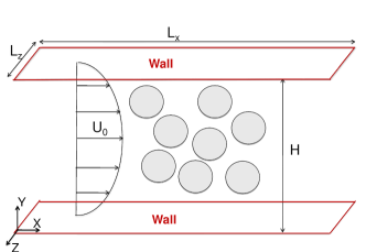
Figure 1: (color online) A schematic of the problem set up.

II.1 Fluid velocity calculation: Boundary integral method

We consider a suspension of fluid-filled deformable Neo-Hookean capsules between two parallel plates as shown in Fig. (1). Both the suspending fluid and the fluid inside the capsules are assumed to be Newtonian and incompressible with the same viscosity, $\mu$, i.e. the viscosity ratio $\lambda$ is unity. We further assume that the Reynolds number for the problem is sufficiently small that the fluid motion is governed by the Stokes equation. Under these assumptions, one may write the fluid velocity $\mathbf{u}$ at any point $\mathbf{x}_{0}$ in the domain as (Pozrikidis, 1992):

$$u_{j}(\mathbf{x}_{0})=u_{j}^{\infty}(\mathbf{x}_{0})-\displaystyle\frac{1}{8\pi\mu}\displaystyle\sum_{n=1}^{N_{p}}\int_{S^{n}}\Delta f_{i}(\mathbf{x})\,G_{ji}(\mathbf{x}_{0},\mathbf{x})\,dS(\mathbf{x})$$ (1)

where $\mathbf{u}^{\infty}(\mathbf{x}_{0})$ is the undisturbed pressure driven velocity at point $\mathbf{x}_{0}$, $S^{n}$ denotes the surface of particle $n$, $\Delta\mathbf{f}(\mathbf{x})$ is the hydrodynamic traction jump across the interface, while $\mathbf{G}$ is the Green’s function for the Stokes equation in the geometry of interest. Note that the sum in the above expression is over all the $N_{p}$ particles in the system. A crucial aspect of the above formulation is that the Green’s function $\mathbf{G}$ is taken to satisfy the boundary conditions imposed at the system boundaries, so the integrals above only involve the internal (interfacial) boundaries; if the Green’s function for any other geometry is employed (e.g. free-space), additional integrals over the domain boundaries will arise in Eq. (1). For the present case of a slit geometry, we have periodic boundary conditions in $x$ and $z$ directions with spatial periods $L_{x}$ and $L_{z}$, respectively (Fig. 1). In the $y$ direction, we have no slip velocity boundary conditions at the two walls at $y=0$ and $y=H$ (Fig. 1).

Traditional implementations of the boundary integral method typically have a scaling of at least $O(N^{2})$, where $N$ is proportional to the product of number of particles $N_{p}$ and the number of elements $N_{\Delta}$ employed to discretize the particle surface. In the present effort, we employ an accelerated implementation of the boundary integral method with a computational cost of $O(N\log N)$ for the slit geometry (Kumar and Graham, 2011). The acceleration in our implementation is provided by the use of the General Geometry Ewald like method (GGEM) (Hernandez-Ortiz et al., 2007), which essentially provides fast solution for the velocity and the pressure fields driven by a collection of point forces in an arbitrary geometry – finding these velocity and pressure fields is at the heart of the solution procedure of the boundary integral method (Kumar and Graham, 2011). The key aspect of the GGEM methodology is to split a Dirac-delta force density into a smooth quasi-Gaussian global density $\rho_{g}(\mathbf{r})$ and a second local density $\rho_{l}(\mathbf{r})$; these are respectively given by the following expressions:

$$\rho_{g}(\mathbf{r})=\frac{\alpha^{3}}{\pi^{3/2}}e^{-\alpha^{2}r^{2}}\left(\frac{5}{2}-\alpha^{2}r^{2}\right),$$ (2a)

$$\rho_{l}(\mathbf{r})=\delta(\mathbf{r})-\rho_{g}(\mathbf{r}),$$ (2b)

where $\alpha^{-1}$ represents a length scale over which the delta-function density $\delta(\mathbf{r})$ has been smeared using the quasi-Gaussian form above, while $\mathbf{r}$ is position vector relative to the pole of the singularity. It is important to emphasize that the total density remains a $\delta$-function, i.e. $\rho_{g}(\mathbf{r})+\rho_{l}(\mathbf{r})=\delta(\mathbf{r})$. The solution associated with a local density, which is known analytically, is short ranged, and is neglected beyond a length scale of $O(\alpha^{-1})$ from its pole. We note that the local solution is obtained assuming free-space boundary conditions. The solution associated with the global density is numerically computed, while ensuring that the boundary conditions associated with the overall problem are satisfied (Hernandez-Ortiz et al., 2007; Kumar and Graham, 2011). Complete details of this method can be found in (Kumar and Graham, 2011); in short, for the slit geometry of interest here we have implemented a spectral Galerkin scheme with Fourier series representation in the periodic $x$ and $z$ directions and Chebyshev polynomial series representation in the $y$ direction; the number of corresponding modes employed in $x$, $y$, and $z$ directions are denoted by $N_{x}$, $N_{y}$, and $N_{z}$, respectively. An important parameter controlling the error of the GGEM solution is $\alpha h_{m}$, where $h_{m}$ is the mean mesh spacing associated with the global solution procedure (e.g. $h_{m}=L_{x}/N_{x}$). Based on extensive tests in (Kumar and Graham, 2011), we have set $\alpha h_{m}=0.5$ in this study with the mean mesh spacing being equal in all three directions. The value of $\alpha$ was held constant in all cases: $\alpha=4/a$, where $a$ is the radius of the spherical capsules at rest.

II.2 Surface discretization and membrane mechanics

The surface of each of the particles is discretized into $N_{\Delta}$ triangular elements with linear basis functions employed over each element. In the present study, we took $N_{\Delta}=320$. As will be seen later, long simulations are required to reach a steady state, and this mesh resolution keeps the computational time requirement manageable. All simulations reported here were performed on a single processor.

The computation of the boundary integral in Eq. (1), requires the knowledge of the hydrodynamic traction jump across the interface ($\Delta\mathbf{f}$). This jump in traction is obtained from the membrane equilibrium condition, which requires that the hydrodynamic forces on any infinitesimal area of the membrane be balanced by the elastic forces in the membrane (Pozrikidis, 1992). Hence $\Delta\mathbf{f}$ can be obtained from the knowledge of elastic stresses. The capsule membrane is modeled here as a neo-Hookean membrane with a shear modulus $G_{s}$ (Barthes-Biesel et al., 2002). The elastic forces in the membrane are then computed using the approach of Charrier et al. (1989), which is based on the principle of virtual work. Implementation details of this approach can be found in (Kumar and Graham, 2011; Pranay et al., 2010).

II.3 Physical parameters

We detail here the various physical parameters relevant for this study. To begin, we note that the rest shape of all capsules is spherical with radius $a$. This radius $a$ will be taken as the unit of length throughout this work. Next, we introduce the undisturbed pressure driven flow, whose velocity in the flow direction $x$ is given by:

$$u=4U_{0}\;\frac{y}{H}\;\left(1-\frac{y}{H}\right),$$ (3)

where $U_{0}$ is the centerline velocity. Based on this flow profile, we obtain a wall shear rate of $\dot{\gamma}_{w}=4U_{0}/H$. Time in this work will be presented in units of $\dot{\gamma}_{w}^{-1}$. The shear modulus of the capsule will be expressed by the non-dimensional capillary number $\mathrm{Ca}=\mu\dot{\gamma}_{w}a/G_{s}$, where $\mu$ is the viscosity of the suspending fluid. The capillary number can be viewed as the ratio of viscous and elastic stresses on the capsule. Since we study suspensions of binary mixtures of capsules with different rigidity, we remark that in a given flow, the values of $\mathrm{Ca}$ of the different particles are not equal: particles with the lower $G_{s}$ have a higher $\mathrm{Ca}$ and are termed floppy particles, while particles with the higher $G_{s}$ have a lower $\mathrm{Ca}$ and are termed stiff particles. The ratio of the rigidities ($G_{s}$) of the stiff particle and the floppy particle will be denoted by $R$, with $R\geq 1$. Another important parameter characterizing a binary mixture is the number fraction of one of species in the suspension – in this work, we employ the number fraction of the floppy particles $X_{f}$. The number fraction of the stiff particles can be obtained from $X_{f}$ as: $X_{s}=1-X_{f}$. The suspension as a whole is characterized by its volume fraction $\phi$, so for example $X_{f}\phi$ is the overall volume fraction of floppy particles.

In the present work, we have neglected bending resistance of the capsule membranes. In such a case, compressive stresses in the membrane can lead to membrane buckling at both at low and high $\mathrm{Ca}$ (Lac et al., 2007). In the buckled state, the numerical result is likely spurious and does not represent true physics. A simple way to alleviate this problem is to introduce an isotropic prestress in the membrane, which can also arise naturally in experiments due to osmotic effects (Sherwood et al., 2003). As a result of the prestress, the rest radius of the capsule $a$ is larger than the unstressed radius $a_{0}$. The degree of inflation can be characterized by the inflation ratio $beta=a/a_{0}-1$. In pair collision studies, inflation ratios between $0.05-0.1$ are typically required to prevent buckling depending on the $\mathrm{Ca}$, though, at higher $\mathrm{Ca}$ even these inflation ratios are insufficient (Lac et al., 2007). In this work, we set the inflation ratio to $\beta=0.1$. We did not observe any buckling instability in our simulations. The effect of preinflation on the cross-stream displacement in pair collisions is usually weak (Lac et al., 2007). We emphasize that the inflated radius $a$ is taken as the relevant radius of the capsule; for example, $\mathrm{Ca}$ is defined based on the inflated radius $a$.

Table 1: Parameter specification in various simulation sets.

Set	$\mathrm{Ca}_{1}$	$\mathrm{Ca}_{2}$	$R$	$X_{f}$	$\phi$	$2a/H$	$N_{p}$
A	0.2	0.5	2.5	0 – 1	0.2	0.197	50
B	0.2	0.5	2.5	0 – 1	0.2	0.3	50
C	0.2	0.5	2.5	0 – 1	0.12	0.197	30
D	0.1	0.6	6.0	0 – 1	0.12	0.197	30

Having defined all the important parameters, we next tabulate the set of simulations performed in this study with their specific choices of parameters (Table 1). As can be seen, we have performed four main sets of simulations, denoted A, B, C and D in the table. These sets of simulations address the effect of the number fraction of the floppy particle $X_{f}$ on the segregation behavior in combination with several other parameters including $\phi$, $\mathrm{Ca}$, $R$ and the confinement ratio $2a/H$.

II.4 Simulation details

We next outline the major steps involved in the solution procedure. The first step involves the computation of the hydrodynamic traction jump $\Delta\mathbf{f}$ – this is computed using the approach outlined above in Sec. (II.2). Following this, we compute the velocity at all surface element nodes employing a discretized version of the boundary integral Eq. (1) (Kumar and Graham, 2011). The surface element nodes are then advanced in time using the second order explicit Adams-Bashforth method. The time step $\Delta t$ is set adaptively to satisfy: $\Delta t=0.5\,Ca\,h$, where $h$ is the minimum node-to-node distance (the nearest nodes do not have to be on the same particle). Recall that time is expressed in units of $\dot{\gamma}_{w}^{-1}$, while distances are expressed in units of $a$. Although the above choice of time step $\Delta t$ is sufficiently small in general, occasional particle-particle overlaps can occur. In principle the time step can be reduced further until overlaps are eliminated, but the computational cost can become exorbitant. Alternatively, the overlaps can be prevented by employing a short range repulsive force, though this is not very effective in three dimensional simulations (Zhao et al., 2010). The best approach appears to be an overlap correction in an auxiliary step (Zhao et al., 2010). This approach is also frequently used in suspensions of rigid particles (Meng and Higdon, 2008; Kumar and Higdon, 2010). In the present work, like in suspensions of rigid particles (Meng and Higdon, 2008), we not only correct the overlaps, but also maintain a minimum gap ($\delta_{min}$) between the surfaces of two particles. In the present case, we set the minimum gap to a small value of one percent of the (rest) particle diameter, i.e. $\delta_{min}=0.02a$. Maintaining the minimum gap is also justified in the absence of adaptive meshing, as that will be necessary to accurately resolve the flow dynamics in the small gaps. No adaptive meshing was employed in this work. The overlap correction procedure involves moving a pair of overlapping particles apart along their line of centers like a rigid particle until the minimum gap requirement is satisfied. Translating the capsules like a rigid particle in this auxiliary step has the benefit that the shapes of the particles remain unchanged, as is the orientation of the particles with respect to the flow. In general, multiple steps of the correction procedure are required, as the correction of overlap between one pair could result in other overlaps (Meng and Higdon, 2008). This overlap correction step involves minimal displacement of the particles, on the order of $\delta_{min}$. Given that the maximum volume fraction studied in this work is $\phi=0.2$, this procedure was rarely required – only a couple of minimum gap violations were observed per time unit. Time integrations were performed for sufficiently long times (hundreds of time units) to allow development of an statistical steady state in the particle distribution.

III Results

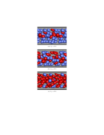
Figure 2: (color online) Simulation snapshots in the shear plane ($x-y$) for different values of $X_{f}$. The snapshots show approximately 1.5 times the length of the simulation box in the $x$ direction. The stiffer particles are light (blue online), while the floppy particles are dark (red online).

We begin by discussing the results for simulation set A of table (1). In this set of runs, the stiffer particle has a capillary number of $\mathrm{Ca}=0.2$, while the floppy particle has a capillary number of $\mathrm{Ca}=0.5$, such that the rigidity ratio $R=2.5$. The confinement ratio for this set of runs was fixed at $2a/H=0.197$. The number fraction of floppy particles in the mixture ($X_{f}$) was varied between 0 and 1, with $X_{f}=0$ corresponding to a pure suspension of stiff particles ($\mathrm{Ca}=0.2$) and $X_{f}=1$ corresponding to a pure suspension of floppy particles ($\mathrm{Ca}=0.5$). Several simulation snapshots for different values of $X_{f}$ are shown in Fig. (2) to help in visualizing the problem set up. We also remark that, throughout this article, we will often use the letter ‘S’ to denote stiff particles, and the letter ‘F’ to denote floppy particles.

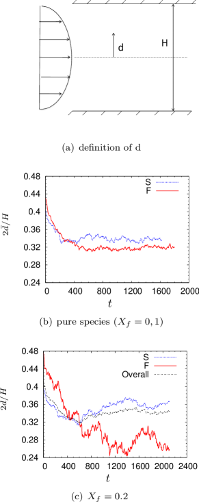
Figure 3: (color online) (a) Definition of d: it gives the absolute distance from the centerline. (b) & (c) Time evolution of the mean absolute distance of a species from the centerline $\bar{d}$ non-dimensionalized by half the channel width $H/2$. In the plots ‘S’ refers to the stiff particles ($\mathrm{Ca}=0.2$), while ‘F’ refers to the floppy particles ($\mathrm{Ca}=0.5$). In (b) results are shown for suspensions of pure species ($X_{f}=0$ & $X_{f}=1$), while in (c) results are shown for a suspension with $X_{f}=0.2$.

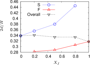
Figure 4: (color online) Steady state $\bar{d}\;$as a function of $X_{f}$ for the $\mathrm{Ca}=0.2$ and $\mathrm{Ca}=0.5$ particles. Also shown is the steady state $\bar{d}\;$of the “overall” suspension.

III.1 Particle distribution in the wall normal direction

The first suspension property we examine is the distribution of particles in the wall normal direction $y$. To characterize this distribution of particles, we will employ three complementary measures. In the first measure, we compute the mean absolute distance of a species from the channel centerline, denoted by $\bar{d}$; see Fig. (3a). This simple measure, though, does not provide detailed information about the actual distribution of particles along the wall normal direction. In order to quantify this distribution, therefore, we will use two additional measures: the first is $\hat{\phi}(y)$, which gives the volume fraction of a given species as a function of $y$-coordinate normalized by the mean volume fraction of that species, while the second measure is $\hat{n}(y)$, which gives the number density of the center of mass of a given species as a function of the $y$-coordinate normalized by the mean number density $n$ of that species. If the distribution were uniform, then both of these measures would have a value of unity throughout. Note that a subscript ‘s’ or ‘f’ may be used with $\hat{\phi}$ or $\hat{n}$ for specifically referring to the stiff or the floppy particles, respectively; the same convention is followed later for denoting other quantities. We now briefly describe the procedure to compute $\hat{n}(y)$; a similar procedure is employed to compute $\hat{\phi}(y)$. For this calculation, the channel height is first divided into bins and then the particles are assigned to bins based on their center of mass coordinates. The number of particles in each of the bins is then normalized by the value expected in that bin based on a uniform distribution in the wall normal direction.

With the different measures for characterizing the particle distribution specified, we turn to the results for these measures. We show the time evolution of $\bar{d}$ for the case of pure species (i.e. $X_{f}=0$ & $X_{f}=1$) in Fig. (3b) and for a mixture with $X_{f}=0.2$ in Fig. (3c). It can be seen that in all cases $\bar{d}$ initially decreases with time, indicating that the particles are drifting toward the centerline. This behavior is not only consistent with results in suspensions of deformable particles subjected to pressure driven flows (Munn and Dupin, 2008; Doddi and Bagchi, 2009), but also with results in suspensions of rigid particles (Phillips et al., 1992; Nott and Brady, 1994). However, as we shall see shortly, the behavior in suspensions of particle mixtures is much richer. In suspensions of pure species (Fig. 3b), we find that $\bar{d}$ reaches an apparent steady state relatively quickly in about $t=500$. In addition, the value of $\bar{d}\;$for stiffer particles ($\mathrm{Ca}=0.2$) is found to be slightly higher than for floppy particles ($\mathrm{Ca}=0.5$), though the difference is not large.

Next, we consider results for the mixture with $X_{f}=0.2$ (Fig. 3c). In this figure, we show $\bar{d}\;$for the stiff particles ($\mathrm{Ca}=0.2$) and the floppy particles ($\mathrm{Ca}=0.2$) individually; in addition, $\bar{d}\;$for the overall suspension is also shown. First of all, one can note that the $\bar{d}\;$for $\mathrm{Ca}=0.2$ particles and $\bar{d}\;$for $\mathrm{Ca}=0.5$ particles are different at $t=0$. This is due to the finite system size with the total number of particles being $N_{p}=50$, and the average being performed over 2 realizations; if large number of realizations are used, then $\bar{d}\;$of both the species will be the same, though this is not expected to affect the steady state distribution. Returning to the figure, we observe that initially both the stiff and the floppy particles drift toward the centerline. However, beyond approximately $t=600$, in what appears to be a slowly evolving process, the stiff particles are displaced toward the walls by the floppy particles. The $\bar{d}\;$of the overall suspension, though, shows much weaker evolution for $t>800$, thereby confirming that this phase of the simulation mostly involves rearrangement of positions between the two particle types. Munn and Dupin (2008) saw a similar behavior in their simulations on mixtures of deformable particles, which led them to the same conclusion as here. The mechanism underlying this observation is described in Sec. (IV).

We next summarize the results for the steady state $\bar{d}\;$of both the species at all values of $X_{f}$ studied here (Fig. 4). Note that the steady state $\bar{d}\;$was obtained by averaging over the last 1000 time (strain) units of the simulation. Two trends are immediately obvious in this plot. First is that $\bar{d}\;$for both the stiff and the floppy particles increase with increasing $X_{f}$, though $\bar{d}\;$for the whole suspension actually decreases with increasing $X_{f}$. The latter is expected as with increasing $X_{f}$, the suspension, on average, becomes more deformable and hence has a lower $\bar{d}\;$. An alternative interpretation of the above observation is that with increasing fraction of the floppy particles, the stiffer particles get displaced toward the wall, while with increasing fraction of the stiffer particles, the floppy particles get displaced toward the centerline. The second observation is on the rate of increase or decrease in $\bar{d}\;$of a given species with changing fraction of the other species: the rate of increase in $\bar{d}\;$of stiffer particles is more rapid with increasing $X_{f}$ than is the rate of decrease in $\bar{d}\;$of floppy particles with decreasing $X_{f}$. This points toward a varying degree of segregation with changing $X_{f}$, which we will quantify shortly with an appropriate measure.

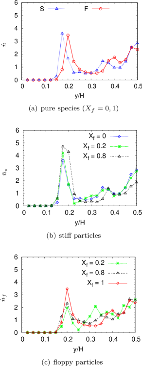
Figure 5: (color online) Number density distribution of a given species in the wall normal direction normalized by the mean number density of that species, $\hat{n}(y)$. The channel wall is at $y=0$ and the centerline at $y=0.5H$. Note that a uniform distribution will yield a value of one throughout. (a) Pure species: $X_{f}=0$ & $X_{f}=1$, (b) $\hat{n}_{s}(y)$ for stiff particles at various values of $X_{f}$, and (c) $\hat{n}_{f}(y)$ for floppy particles at various values of $X_{f}$.

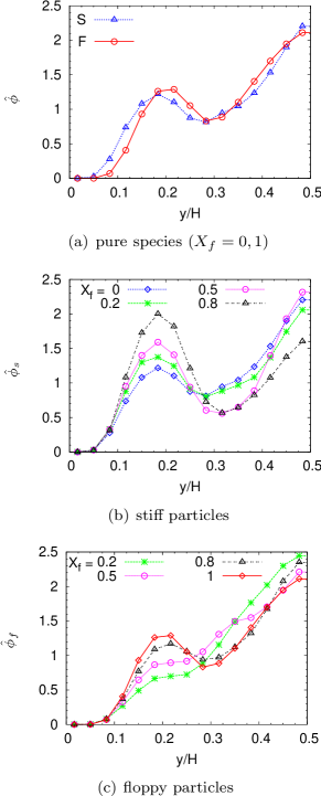
Figure 6: (color online) Volume fraction distribution of a given species in the wall normal direction normalized by the mean volume fraction of that species, $\hat{\phi}(y)$. The channel wall is at $y=0$ and the centerline at $y=0.5H$. A uniform distribution will yield a value of one throughout. (a) Pure species: $X_{f}=0$ & $X_{f}=1$, (b) $\hat{\phi}_{s}(y)$ for stiff particles at various values of $X_{f}$, and (c) $\hat{\phi}_{f}(y)$ for floppy particles at various values of $X_{f}$.

To gain further insights into the particle distribution, Figs. (5) and (6) show $\hat{n}(y)$ and $\hat{\phi}(y)$, respectively. Note that in these figures, the channel wall is at the left and the centerline at the right – results in each half of the slit have been combined to enhance the statistics. We first examine Fig. (5a), which shows $\hat{n}(y)$ for suspensions of pure species ($X_{f}=0$ and $X_{f}=1$). In this plot two peaks are very apparent: a sharp peak close to the wall and a broad peak close to the centerline. Even though the peak close to the wall looks sharper in comparison to the one at the centerline, the width of this peak is relatively small; hence the volume fraction around the sharp peak is much lower in comparison to the volume fraction around the centerline (Fig. 6a). Also, the peak next to the wall is closer to it for the stiffer particles than for the floppy particles, thereby indicating that the cell free layer is wider in suspensions of more deformable particles consistent with other simulations (Doddi and Bagchi, 2009). The presence of peaks also points toward the formation of layers, though particle snapshots (see Fig. 2) and animations reveal that only the peaks near the walls are representative of layers, while much of the interior region consists of disorganized particles. This is similar to observations is confined suspensions of drops (Li and Pozrikidis, 2000). The layering close to the walls in concentrated suspensions is easily explained by recalling that the wall is a no penetration boundary, thereby promoting the formation of layers next to it. It is also worth pointing out that the volume fraction at the centerline (Fig. 6a) is about twice the average volume fraction. Hence the suspension is concentrated around the centerline with the volume fraction there being $\phi\approx 0.4$.

We next examine the effect of varying $X_{f}$ on $\hat{n}(y)$ and $\hat{\phi}(y)$ of individual species. We focus first on the stiff particles, for which $\hat{n}_{s}(y)$ is shown in Fig. (5b) and $\hat{\phi}_{s}(y)$ in Fig. (6b). It is clearly seen that with increasing fraction of floppy particles, the concentration of stiff particles increases in the near wall region; at low values of $X_{f}$ this increase is mostly compensated by the decrease in concentration in the region between the two peaks (one at the centerline and one next to the wall), while at higher values of $X_{f}$, the stiffer particles are also slightly depleted in the region around the centerline. For the floppy particles (Fig. 5c and 6c), the exact opposite behavior is observed, namely, with increasing fraction of stiffer particles (i.e. decreasing $X_{f}$), floppy particles get depleted in the region close to the walls and accumulate in the region between the two peaks; no significant changes in the concentration are observed in the region close to the centerline, except at very low values of $X_{f}$.

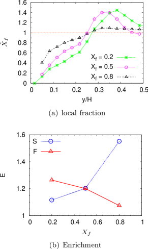
Figure 7: (color online) (a) Local fraction of the total particle volume contributed by floppy particles normalized by its bulk value, $\hat{X}_{f}$. (b) The enrichment factor $E$ for both floppy (F) and stiff (S) particles as a function of $X_{f}$.

We turn now to quantifying the degree of segregation in the mixture. Here, we employ a particularly simple measure based on the volume fraction distribution of the two species as a function of the wall normal coordinate. To begin with, we compute $\tilde{X}_{f}(y)$ defined as the fraction of the total particle volume contributed by floppy particles as a function of the wall normal coordinate:

$$\tilde{X}_{f}(y)=\frac{\phi_{f}(y)}{\phi_{s}(y)+\phi_{f}(y)}.$$ (4)

This fraction normalized by the mean number fraction of the floppy particles $X_{f}$ is denoted by $\hat{X}_{f}(y)$: $\hat{X}_{f}(y)=\tilde{X}_{f}(y)/X_{f}$, which essentially gives the local enrichment (when $\hat{X}_{f}(y)>1$) or depletion (when $\hat{X}_{f}(y)<1$) of the floppy particles. We show in Fig. (7a) the plot of $\hat{X}_{f}$ as a function of the wall normal coordinate ($y$) for various values of $X_{f}$. As expected, in all cases, floppy particles are enriched in the region close to the centerline, while the stiffer particles are enriched in the region close to the walls. If one’s goal is to separate these two species, then an obvious way to achieve this is by separating the suspension present in these two regions. In this particular case, the plane separating these two regions is found to be $y\approx H/4$. We then define an enrichment factor $E$ for each species as the ratio of its fractional contribution to the total particle volume in its enriched region normalized by the corresponding bulk value. For example the enrichment factor for floppy particles $E_{f}$ is obtained as

$$E_{f}=\frac{1}{X_{f}}\left(\;\frac{\int\phi_{f}(y)dy}{\int(\phi_{s}(y)+\phi_{f}(y))dy}\right),$$ (5)

where the integrals in the above equation are restricted to the region where $\hat{X}_{f}\geq 1$. We remark that, by definition, $E\geq 1$. We show the plot of $E$ for both species as a function of the mean fraction of the floppy particles $X_{f}$ in Fig. (7b). This result shows that the enrichment of either species increases as it becomes more dilute. Moreover, the rate of this increase is much more rapid for the stiffer particles than for the floppy particles. This slow increase for the floppy particles is perhaps not too surprising, as its enriched region is centered around the centerline, where even the stiffer particles have a propensity to accumulate, thereby reducing the relative enhancement of the floppy particles.

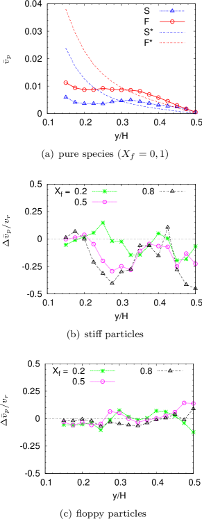
Figure 8: (color online) (a) Average velocity $\bar{v}_{p}\;$of a particle of a given type in suspensions of pure species (S & F) as a function of $y$. Also shown are the velocities of an isolated (single) stiff (S*) and floppy (F*) particles in the same geometry and flow. (b) Relative change in the velocity of the stiff particles at a given $X_{f}$ over the corresponding pure species result in (a). (c) Same as (b), but for the floppy particles.

III.2 Particle velocity in the wall normal direction

So far we have focused on the particle distribution in the wall normal direction. It will also be of great interest to examine the particle velocity in the wall normal direction, as that is expected to play an important role in its distribution in the wall normal direction. We first show, in Fig. (8a), the mean wall normal particle velocity $\bar{v}_{p}(y)$ in suspensions of pure species ($X_{f}=0$ and $X_{f}=1$). This is obtained by first dividing the channel height into bins. A given particle’s instantaneous wall normal velocity is then assigned to a bin based on the wall normal coordinate of its center of mass; the average velocity in a bin then gives the $\bar{v}_{p}$ in Fig. (8a). For comparison, we also plot in the figure the quasi-steady wall normal velocity of an isolated capsule. This quasi-steady velocity is obtained by holding the center of mass of the isolated particle steady at a given location – at the end of each timestep, the particle was translated so that its center of mass returned to the original position. The resulting steady state particle velocity is referred to as the isolated particle quasi-steady migration velocity.

The mean particle velocity $\bar{v}_{p}$ in the suspension appears to show three different regimes (Fig. 8a). In the region close to the walls ($y/H<0.2$), $\bar{v}_{p}$ is a decreasing function of the distance from the walls, much like the migration velocity of an isolated particle, though the velocity in the suspension is significantly lower. Recall that $y/H=0.2$ approximately corresponds to the peak of $\hat{n}(y)$ and $\hat{\phi}(y)$ (Figs. 5 & 6). In the intermediate region ($0.2H<y<0.3H$), $\bar{v}_{p}$ is approximately a constant, and can even be a slightly increasing function of distance from the wall$y$. In the region close to the centerline ($0.3H<y<0.5H$), the velocity decreases linearly with distance. This behavior is similar to that of an isolated particle, whose migration velocity close to the centerline also decreases linearly with distance. This results from the fact the shear rate decreases linearly with distance in Poiseuille flow, while the gradient of the shear rate is a constant. The migration velocity, which, to leading order near the centerline, is the product of these two terms, therefore decreases linearly with distance (Leal, 1980). Perhaps the most interesting feature in Fig. (8a) is the fact the mean particle velocity in the suspension can be higher than the corresponding isolated particle migration velocity. This effect certainly arises due to particle-particle interactions and is discussed further below.

We next turn to the effect of $X_{f}$ on $\bar{v}_{p}$ of particles of a given species in the suspension. To quantify this, we compute the relative change in the velocity $\Delta\bar{v}_{p}/v_{r}=(\bar{v}_{p}-v_{r})/v_{r}$, where $v_{r}$ refers to $\bar{v}_{p}$ in the corresponding pure species suspension. We show plots of $\Delta\bar{v}_{p}/v_{r}$ for the stiff particles at several values of $X_{f}$ in Fig. (8b), while the same plots for the floppy particles are shown in Fig. (8c). Focusing first on the stiff particles, we find that their mean wall normal velocity $\bar{v}_{p}$ is greatly reduced, in some cases by nearly $50\%$, as the fraction of floppy particles in the suspension increases. The most significant decrease in the velocity is observed in the second region discussed above, where $\bar{v}_{p}$ of the particles in suspensions of pure species is approximately a constant (Fig. 8a). A significant decrease is also observed in a thin region around the centerline, though, $\bar{v}_{p}$ itself is very small here. To gain some insights into this behavior, we remark that with increasing fraction of the floppy particles, a stiff particle is expected to “collide” more frequently with floppy particles than with particles of the same kind, particularly from its side facing the centerline where most of the floppy particles are concentrated. Therefore, it appears that the mean additional effect of these heterogeneous collisions is to push the stiffer particles toward the wall. Later, in Sec. (IV), it will be shown that this observation is consistent with simple model studies on homogeneous and heterogeneous pair collisions. We next consider the effect of $X_{f}$ on $\bar{v}_{p}$ of floppy particles (Fig. 8c). It is immediately obvious that, in comparison to $\bar{v}_{p}$ of stiffer particles, $\bar{v}_{p}$ of floppy particles is a weak function of $X_{f}$ and no particular conclusion can be drawn based on these trends.

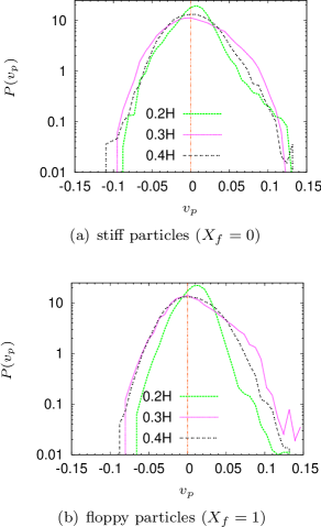
Figure 9: (color online) Probability distribution of the wall normal particle velocity $v_{p}$ at several values of $y/H$. (a) pure stiff particles ($X_{f}=0$), and (b) pure floppy particles ($X_{f}=1$).

Above, we examined the mean particle velocity $\bar{v}_{p}$. This particle velocity also exhibits considerable fluctuations about this mean. To emphasize this, we show in Fig. (9) the probability distribution of particle velocities $P(v_{p})$ on a log-linear scale at various wall normal coordinates in suspensions of pure stiff and floppy particles, i.e. $X_{f}=0$ and $X_{f}=1$, respectively. Not only do these plots confirm that there are considerable fluctuations in particle velocity (this is quantified below), but the exact nature of these distributions is interesting in itself and deserves a brief discussion. Perhaps the most interesting observation in these plots is that the distribution of positive velocities for particles close to the wall ($y=0.2H$ in the figure) is non-Gaussian, and is, in fact, much closer to an exponential distribution. At larger values of $y/H$, this changes to a Gaussian distribution. In contrast, the distribution of negative velocities appears to be Gaussian at all values of $y/H$. Since one usually expects a Gaussian distribution for a variable that is obtained as a sum of many uncorrelated parts (in view of the central limit theorem (Gardiner, 2004)), the appearance of an exponential distribution perhaps implies contributions from correlated parts (Drazer et al., 2002). In the present case, the underlying physics of the problem provides a basis for these observations. We note that a particle is expected to show a non-zero wall normal velocity both due to “random” collisions (interactions) with its neighbors, as well as due to the non-random effects of the shear rate gradient and hydrodynamic wall repulsion (Leal, 1980; Smart and Leighton, 1991). In light of the above discussion, therefore, the former contribution can be expected to lead to a Gaussian distribution, while the latter to a non-Gaussian one. Since both the shear rate gradient and wall repulsion lead to positive velocities, it is therefore not surprising that one observes a non-Gaussian positive velocity distribution, especially close to the walls where the non-random effect is dominant. Negative velocities, on the other hand, can result only due to interactions of a particle with its neighbors, and therefore can be expected to have a Gaussian distribution.

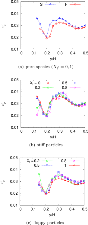
Figure 10: (color online) Fluctuation (standard deviation) of the particle velocity of a given species as a function of $y/H$. (a) In suspensions of pure species ($X_{f}=0$ & $X_{f}=1$), (b) for stiffer particles at various values of $X_{f}$, (c) for floppy particles at various values of $X_{f}$.

We next quantify the fluctuation in the particle velocity by computing its standard deviation, denoted by $v^{\prime}_{p}$. We first show in Fig. (10a) plots of $v^{\prime}_{p}$ as a function of $y$ in suspensions of pure species. As can be seen, the fluctuations in the velocity are much larger than the corresponding mean, especially in the region close to the centerline. This is particularly true for the stiff particles as they not only show a smaller $\bar{v}_{p}$, but also a higher $v^{\prime}_{p}$. We also find in the plot that the fluctuations show a minimum in the region near the wall ($y\approx 0.2H$). This minimum in fluctuation appears to result from the orderly motion of particles in the layer formed next to the wall (Fig. 6a). Moving further away from the wall, we observe a maximum in the fluctuation $v^{\prime}_{p}$ at approximately $y=0.3H$. This position corresponds well with the minimum in $\hat{\phi}(y)$ in Fig. (6). The maximum in the fluctuation implies that a particle at this position undergoes more frequent collisions with other particles than do particles at neighboring positions, and hence a particle in this region is expected to drift away from this region. It is not surprising, therefore, that the position of the maximum in velocity fluctuation corresponds well with the minimum in $\hat{\phi}(y)$. In addition, we observe that the fluctuation amplitude in the region close to the centerline is non-zero, and stays finite even at the centerline ($y=0.5H$) where the local shear rate is zero. This is a well known result in monodisperse suspensions and has been attributed to non-local effects due to the finite particle size (Nott and Brady, 1994; Zhao and Shaqfeh, 2011).

We next summarize the effect of $X_{f}$ on the velocity fluctuations of the stiffer particles in Fig. (10b), and for the floppy particles in Fig. (10c). These plots show that the velocity fluctuation is a weak function of $X_{f}$, though, in general, the fluctuations were higher in mixtures than in the corresponding suspensions of pure species. We also point out that the fluctuations in the velocity of stiffer particles was always higher than the corresponding fluctuations in the velocity of floppy particles.

Based on the particle velocity fluctuations above, which in turn are rooted in particle collisions, one may explain the enhancement in $\bar{v}_{p}$ of a particle in the suspension over the corresponding isolated particle near the centerline (Fig. 8a). Because of the variation in the velocity fluctuations (collisions) as a function of $y$, one can expect a particle to drift down the gradient of velocity fluctuations (collision) (Phillips et al., 1992; Kumar and Higdon, 2011); the velocity fluctuation profile in Fig. (10a) then implies a drift toward the centerline due to this effect, thereby leading to an enhancement in the $\bar{v}_{p}$.

Results with other simulation parameters in Tb. (1) show a qualitatively similar behavior and are presented in the appendix for completeness. In the following section, we explore the mechanism responsible for the segregation behavior.

IV Development of mechanistic model

In this section, we elucidate the mechanism that leads to the segregation between the stiff and the floppy particles in suspensions of mixtures. In particular, we seek to explain the following two observations on the segregation behavior: (i) in a suspension of primarily floppy particles (i.e. large $X_{f}$), the stiff particles accumulate in the near wall region, while being depleted in the region around the centerline, and (ii) in a suspension of primarily stiff particles, the floppy particles are depleted from the near wall region accompanied by an increased accumulation in the region near the centerline. In these statements, the degree of depletion and excess of a given species in a particular region is with respect to the distribution of that species in its pure suspension (i.e. $X_{f}=0$ or $X_{f}=1$). We will show that these observations can be qualitatively explained with a unified mechanism incorporating the wall-induced migration of deformable suspended particles away from the wall and the particle fluxes associated with heterogeneous and homogeneous pair collisions.

IV.1 Framework

To make progress toward elucidating the segregation mechanism, it will be helpful to first develop a modeling framework with which to analyze and interpret the simulations results. In particular, we focus on the particle motion in the wall normal direction and identify the distinct mechanisms that result in such a motion.

An isolated deformable particle in a pressure driven flow acquires a non-zero wall normal migration velocity both due to hydrodynamic interactions with the walls (wall repulsion) (Smart and Leighton, 1991) and due to the curvature in the flow profile (shear rate gradient) (Leal, 1980). In Sec. (III), we presented the quasi-steady migration velocity of an isolated capsule in Poiseuille flow; see Fig. (8). For the present section, we denote this velocity by $V^{S}$, where the superscript ‘S’ signifies the origin as the single (isolated) particle motion.

In a suspension of particles, the interparticle interactions also contribute to the particle’s wall normal drift velocity (Li and Pozrikidis, 2000). In general, developing exact expressions for the particle velocity in the suspension is difficult, although for dilute solutions the treatment is relatively simple. This will prove sufficient for our present, qualitative purposes. In the dilute limit, as an approximation, we can sum velocity contributions resulting from the isolated particle motion and due to contributions from particle interactions treated in a pairwise fashion. The neglect of three-particle and higher order interactions will cause an error of $O(\phi^{2})$, which is small in dilute suspensions. We will denote the contribution to a particle’s velocity resulting from pair collisions by $V^{P}$, where the superscript ‘P’ signifies the origin of the term being pair collisions. We can combine the contributions from pair collisions and single particle motion to obtain the total wall normal particle drift velocity as:

$$V\;=\;V^{S}+V^{P}.$$ (6)

We next develop an expression for the velocity of a particle resulting due to pair collisions ($V^{P}$).

The (ensemble-averaged) velocity of a particle arising due to pair collisions in a dilute suspension can be expressed by a precise integral expression; see, e.g., Li and Pozrikidis (2000). For our qualitative discussion in the present work, however, we employ and expand on the much simpler phenomenological model of Phillips et al. (1992). In this model, the number of collisions experienced by a test particle is taken to scale as $\dot{\gamma}\phi$. The variation of this collision frequency over a distance of $O(a)$ is then given by $a\nabla(\dot{\gamma}\phi)$, where $\nabla$ here reduces to the derivative with respect to $y$. Furthermore, each of these collisions are assumed to cause a displacement of $O(a)$, thereby leading to a particle velocity given by:

$$V^{P}=-Ka^{2}\nabla(\dot{\gamma}\phi),$$ (7)

where $K$ is a dimensionless constant that may depend on the properties of the particles in the suspension (e.g. capillary number, shape). A few words are in order about the interpretation of this parameter. We note that the above expression was derived under the assumption that the particle undergoes a displacement of $O(a)$ in pair collisions, which is an appropriate order of magnitude estimate, though it does not provide precise information about the actual characteristic displacement in pair collisions. This information takes additional significance when considering a suspension of mixtures, as the characteristic displacement in pair collisions is expected to be different when a test particle undergoes collision with a particle of the same type (homogeneous collision) or with a particle of the other type (heterogeneous collision). Furthermore, the characteristic displacement will also depend on the identity of the test particle, i.e. whether it is stiff or floppy. In order to make the above model (Eq. 7) cognizant of this information, we view ‘$K\,a$’ as the characteristic displacement of a particle in pair collisions. For example, when considering pair collisions between smooth rigid spheres, we have $K=0$ as the characteristic displacement in such collisions vanishes owing to the symmetry of the geometry and the Stokes flow reversibility. With this aspect clarified, we generalize Eq. (7) for a suspension of mixtures to obtain:

$$V_{s}^{P}=-a^{2}\left(K_{ss}\nabla(\dot{\gamma}\phi_{s})+K_{sf}\nabla\,(\dot{\gamma}\phi_{f})\right),$$ (8a)

$$V_{f}^{P}=-a^{2}(K_{fs}\nabla(\dot{\gamma}\phi_{s})+K_{ff}\nabla(\dot{\gamma}\phi_{f})),$$ (8b)

where the subscript ‘s’ and ‘f’ denote the stiff and the floppy particle, respectively. We next discuss results from several pair collision studies as they provide important insights into the relative values of the characteristic displacements in various scenarios, i.e. it provides information about the relative values of the various constants $K$ in equation (8).

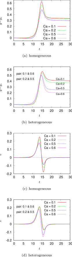
Figure 11: (color online) Pair collisions: Displacement of a particle relative to its initial position ($y-y_{i}$) with time in (a) homogeneous pair collisions and (b) heterogeneous pair collisions. Wall normal velocity of a particle as a function of time in (c) homogeneous pair collisions and (d) heterogeneous pair collisions.

IV.2 Pair collisions

We presented above the particle velocity resulting from pair collisions between particles, which obviously plays an important role in the particle distribution along the wall normal direction. To gain more insights into this process, it will be helpful to examine some pair collision results, particularly for pair collisions between two different species, as no prior study appears to have addressed this problem. We begin by describing the problem setup for pair collision studies. In all studies, a large cubic simulation box of side $30a$ was considered, and the particles were placed on either side of the central plane with a given initial separation. Further, in all these studies, only simple shear flows were considered. These choices for the problem setup minimize the single particle migration effect, and hence provide insights into the effect of particle-particle interactions (collisions).

We begin by considering pair collisions between the same species (homogeneous collisions) and show in Fig. (11a) the displacement of the ‘top’ particle in the wall normal direction relative to its initial position ($y-y_{i}$) as a function of time. For this study and those below, we set the initial separation between the two particles in the wall normal direction as $\Delta y_{i}=0.5a$. Other studies with $\Delta y_{i}=0.25a$ and $\Delta y_{i}=0.75a$ gave similar trends. In the above figure, it is clearly seen that in this range of $\mathrm{Ca}$ ($0.1\leq\mathrm{Ca}\leq 0.6$), the final displacement ($\delta_{\infty}=y_{\infty}-y_{i}$) increases with decreasing $\mathrm{Ca}$. We remark that $\delta_{\infty}$ is known to be a non-monotonic function of $\mathrm{Ca}$, such that at low enough enough $\mathrm{Ca}$, $\delta_{\infty}$ decreases with decreasing $\mathrm{Ca}$ (Pranay et al., 2010).

We next consider collisions between two particles with different $\mathrm{Ca}$ (Fig. 11b). From these results we see that the stiffer particle undergoes much larger displacement ($\delta_{\infty}$) than the corresponding floppy particle involved in the collision. In addition, the difference in the final displacements of the two species is larger for larger rigidity ratio system. Further insights are obtained by comparing the instantaneous wall normal velocities of the particles during the collision event for the cases in Figs. (11a) and (11b), which are shown in Figs. (11c) and (11d), respectively. Focusing first on the result for particle velocity in homogeneous pair collisions (Fig. 11c), we find the particle velocity is positive in the approach part of the collision trajectory, while it is negative in the receding part of the collision trajectory. As a result of this feature, a fraction of the maximum displacement in Fig. (11a) is recovered in the receding part of the collision trajectory. It is obvious from Fig. (11c) that the magnitude of velocity in either part of the trajectory is higher for the stiffer particle than the floppy particle in homogeneous collisions. In contrast, in heterogeneous collisions (Fig. 11d), while the magnitude of the velocity is higher for the stiff particle in the approach part of the trajectory, in the receding part it is the floppy particle which exhibits a greater magnitude of velocity. This reversal in the trends of the velocity in the receding part of the trajectory leads to the observed behavior in heterogeneous pair collisions. Summarizing the results of this section, we have the following relationships between the various constants $K$ in Eq. (8): (i) $K_{sf}>K_{fs}$, (ii) $K_{sf}>K_{ss}$, and (iii) $K_{fs}<K_{ff}$. We next discuss the implications of these pair collision results on the segregation behavior.

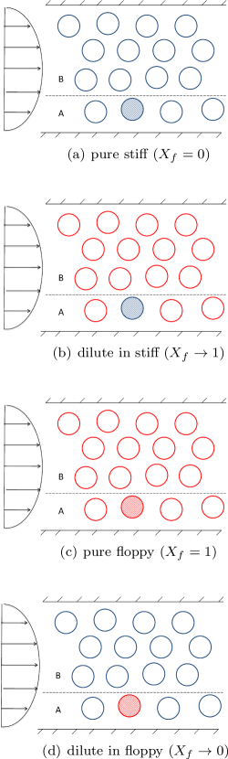
Figure 12: (color online) A cartoon depicting the characteristics of the neighborhood of a particle of given type (shaded) in the near wall region at various values of $X_{f}$. The stiff particle is shown light (blue online), while the floppy particle is shown dark (red online).

IV.3 Mechanism of flow induced segregation

Based on the results of pair collision studies and the single particle migration velocity, we are now in a position to identify the mechanism responsible for the segregation behavior. In a confined suspension, the wall plays an important role as it breaks the translational invariance in the wall normal direction. So, we divide the overall system domain in two parts: first is the near wall region, and second is the interior region. These two regions are pictorially shown in Fig. (12), where the near wall region is labeled as ‘A’, while the interior region is labeled as ‘B’. We first focus on the near wall region as that turns out to be critical to the segregation behavior. For a particle in the near wall region A (e.g., shaded particles in Fig. 12), the net of effect of pair collisions is to push to particle toward the wall, as $-\nabla(\dot{\gamma}\phi)$ is negative in this region. In other words, a particle in this region undergoes collisions with other particles present only on its upper half and consequently gets pushed toward the wall. Therefore, the net effect of these pair collisions is to prevent the ‘escape’ of the particles in the near wall region A to the interior region B. In contrast, the single particle velocity $V^{S}$, which is always toward the centerline, aids the particle in ‘escaping’ to the interior region B. Since the single particle migration velocity $V^{S}$ depends only on the characteristics of the particle, it is independent of $X_{f}$. On the other hand, $V^{P}$, the velocity arising due to pair collisions, depends strongly on $X_{f}$ in view of the results of homogeneous and heterogeneous pair collisions discussed above, i.e. due to differences in values of $K_{ss}$, $K_{ff}$, $K_{sf}$ and $K_{fs}$. Therefore, the frequency with which a particle present in the region A will escape to the region B will depend on $X_{f}$ primarily due to the dependence of $V^{P}$ on $X_{f}$.

To aid in visualizing the problem at various values of $X_{f}$, we consider four cases as shown in Fig. (12): (a) suspension of stiff particles only ($X_{f}=0$), (b) suspension that is dilute in stiff particles ($X_{f}\rightarrow 1$), (c) suspension of floppy particles only ($X_{f}=1$), (d) suspension that is dilute in floppy particles ($X_{f}\rightarrow 0$). In the first two cases, our focus is on the behavior of the stiff particle, while in the last two cases, our focus is on the behavior of the floppy particle; in all cases the particle of interest is shaded. Focusing first on a stiff particle, its velocity $V^{P}$ in cases (a) and (b) is given by $V^{P}=-K_{ss}a^{2}\nabla(\dot{\gamma}\phi)$ and $V^{P}=-K_{sf}a^{2}\nabla(\dot{\gamma}\phi)$, respectively. In Sec. (IV.2), we concluded that $K_{ss}<K_{sf}$, and hence that the stiff particle in case (a) faces a smaller barrier in escaping to region B than the stiff particle in case (b). Therefore, we conclude that a stiff particle gets increasingly localized in the near wall region as the fraction of floppy particles in the suspension increases. We next turn our attention to the behavior of the floppy particle and consider cases (c) and (d) in Fig. (12). The velocity of the floppy particle in these cases is given by $V^{P}=-K_{ff}a^{2}\nabla(\dot{\gamma}\phi)$ and $V^{P}=-K_{fs}a^{2}\nabla(\dot{\gamma}\phi)$, respectively. The results of Sec. (IV.2) indicate that $K_{ff}>K_{fs}$, and consequently that the frequency of escape of the floppy particle to region B from region A should increase as the fraction of stiff particles in the suspension increases.

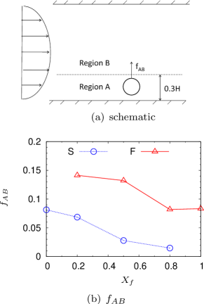
Figure 13: (color online) (a) A schematic defining the near wall region A and the interior region B. (b) Transition probability $f_{AB}$ defined as the fraction of particles starting in region A crossing over to region B in $t=100$. $f_{AB}$ is shown as function of $X_{f}$ for both the stiff and the floppy particles.

To verify the mechanism presented above, we compute the probability of transition of a particle of a given type from region A to region B as a function of $X_{f}$ (Fig. 13b). More precisely, this transition probability, denoted by $f_{AB}$, gives the fraction of particles that are present in region A at a given time, but cross over to region B within 100 time units from that time. We have defined the near wall region A as the region extending to a distance of $0.3H$ from either walls, while the remainder of the domain is defined as region B (Fig. 13a). The choice of $0.3H$ comes from the minimum of $\hat{\phi}$ in Fig. (6a) and $\hat{n}$ in Fig. (5a), which essentially separates the near wall region and the interior region. The transition probability $f_{AB}$ in Fig. (13b) clearly clearly shows trends consistent with the mechanism described above. We focus first on the trends for stiff particles. At $X_{f}=0$, we find $f_{AB}^{s}\approx 0.081$, which gradually decreases to $f_{AB}^{s}\approx 0.015$ at $X_{f}=0.8$, which amounts to a factor of $5.4$ reduction in the transition probability. This result clearly suggests that stiff particles get localized in the near wall region as the fraction of floppy particles increases, which must be due to the effect of pair collisions, as the isolated particle migration velocity is independent of $X_{f}$. As discussed earlier, this is the expected trend based on the relative values of $K_{ss}$ and $K_{sf}$, as $K_{sf}>K_{ss}$. We next focus on the trends of $f_{AB}$ for the floppy particle in Fig. (13b). At $X_{f}=1$, we find $f_{AB}^{s}\approx 0.083$, which gradually increases to $f_{AB}^{s}\approx 0.1413$ at $X_{f}=0.2$, which amounts to a factor of $1.7$ increase in the transition probability. This implies that, with increasing fraction of the stiff particles, the floppy particles escape to the interior region more easily. This again is expected based on the results of pair collisions as $K_{fs}<K_{ff}$.

It is also interesting to note that the $f_{AB}$ for both the stiff and the floppy particles are very close in their corresponding suspensions of pure species, i.e. $X_{f}=0$ and $X_{f}=1$, respectively. Results of pair collisions above indicate that the $K_{ss}$ and $K_{ff}$ are about the same, though the single particle migration velocity $V^{S}$ is larger for the floppy particle. A larger $V^{S}$ for the floppy particle, in principle, should lead to a higher $f_{AB}$ for that particle. On the other hand, a larger $V^{S}$ may lead to more frequent collisions with a relatively smaller $\Delta y_{i}$, the initial separation between the two colliding particles in the wall normal direction, as this velocity will cause two particles to approach each other in the wall normal direction. Since collisions with smaller $\Delta y_{i}$ lead to larger cross stream displacement $\delta_{\infty}(\Delta y_{i})$ (Lac et al., 2007), the effect of larger $V^{S}$ may be nullified by the effect of larger $\delta_{\infty}(\Delta y_{i})$. This effect enters our model through the effect of $\delta_{\infty}(\Delta y_{i})$ on the constant $K$, as the constant $K$ is essentially the weighted average of $\delta_{\infty}(\Delta y_{i})$, where the weight is the probability for a collision with a given $\Delta y_{i}$ to occur. Computing this weighted average rigorously is beyond the scope of the present work.

In addition to the mechanism outlined above, we must also address the effects of excluded volume, which is only expected to amplify the effects of this mechanism. This is because if the floppy particles find it easier to escape to the interior than the stiff particles, then their enhanced presence in the interior will only make the escape of the stiff particles to the interior more difficult, as only a limited volume fraction of particles can be present in the interior. So far we have been treating the motion of stiff particles and floppy particles separately. The excluded volume effect essentially couples the motion of these two species, which is intuitively expected to be the case in a suspension of particles, especially at non-dilute volume fractions.

So far we have focused entirely on the near wall region. We now briefly discuss the dynamics in the interior region. In this region, a particle has near neighbors both in its upper and lower half, and hence the gradient in the collision frequency $a\nabla(\dot{\gamma}\phi)$ is expected to be small relative to the collision frequency $\dot{\gamma}\phi$ itself (the latter collision frequency is only an approximation as it does not account for finite particle size; see Sec. III.2). When coupled with the fact that the single particle velocity is also small far away from the walls (Sec. III.2), we conclude that the particle motion in this region is expected to be dominated by shear-induced diffusion. Therefore, the characteristics of the particle motion in this region are not expected to play a dominant role in the segregation between the two species. Nonetheless, the diffusive behavior in this region is necessary for transporting the particles from the bulk to the near wall region, and hence indirectly plays a role in the observed segregation between the two species.

We conclude this section by addressing an interesting feature concerning the time evolution of the mean absolute distance $\bar{d}\;$of a species in a mixture. In Sec. (III.1), we observed that in a mixture of stiff and floppy particles, $\bar{d}\;$of both species initially decreases with time (Fig. 3c). But, beyond approximately $t=600$ in Fig. (3c), the $\bar{d}\;$of stiff particles was found to gradually increase with time. This phase of the process was termed as a reorganization phase between the stiff and the floppy particles, as $\bar{d}\;$of the overall suspension was essentially steady in this phase of the simulation. Based on the mechanism outlined above, this reorganization phase can be associated with the transport of the stiff particles in the interior region to the near wall region, where they are expected to become nearly irreversibly trapped. Therefore, the time scale after which this reorganization phase is noticeable in simulations can be associated with the time required for a particle near the centerline to diffuse to the near wall region. We therefore see that the mechanism outlined here is capable of addressing even the finer aspects of the segregation behavior.

V Conclusions

In this article we investigated the segregation behavior in suspensions of binary mixtures of Neo-Hookean capsules subjected to pressure driven flow in a planar slit. The two species in the binary mixture have different membrane rigidities as characterized by their separate capillary numbers. Detailed boundary integral simulations revealed that with increasing fraction of the floppy particles in the suspension (i.e. with increasing $X_{f}$), there is an enhancement in the concentration of the stiff particles in the near wall region. On the other hand, as the fraction of stiff particles in the suspension increases (i.e. $X_{f}$ decreases), a depletion in the concentration of floppy particles in the near wall region is observed. As a result of this behavior, stiff particles segregate in the near wall region in a suspension of primarily floppy particles, while floppy particles segregate around the centerline in a suspension of primarily stiff particles. A novel and detailed mechanism based on the degree of localization of a particle of a given type in the near wall region as a function of $X_{f}$ was developed. The three main ingredients of this mechanism which governs the localization of a particle in the near wall region are: (i) the single particle migration velocity toward the centerline, which provides an avenue for the particle to escape to the interior, (ii) the repeated pair collisions of a particle in the near wall region with its neighboring particles, which pushes it toward the wall, thereby preventing its escape to the interior and (iii) the difference in final displacement between homogeneous and heterogeneous pair collisions. The single particle migration velocity is independent of $X_{f}$, while the cross-stream displacement depends strongly on $X_{f}$. In particular, results of heterogenous pair collisions involving a stiff and a floppy particle showed that the stiff particle experiences a substantially larger cross-stream displacement as a result of the collision than the floppy particle. This result indicates, consistent with simulation results, that as the fraction of floppy particles in the suspension increases, a stiff particle in the near wall region will get increasingly localized there due to the strong effect of heterogeneous pair collisions on its wall-normal displacement. On the other hand, as the fraction of stiff particles in the suspension increases, a floppy particle in the near wall region can escape to the interior much more easily due to the much weaker effect of heterogenous pair collisions on its wall-normal displacement. This mechanism, therefore, consistently explains the features of the segregation behavior observed in detailed numerical simulations. Important topics for future work will be the extent to which the same picture can explain segregation by size and shape as well as segregation in the (nominal) absence of shear rate gradients, as in plane Couette flow. It will also be of interest to formalize the qualitative picture into a stochastic process model that more quantitatively captures the simulation and experimental results.

*

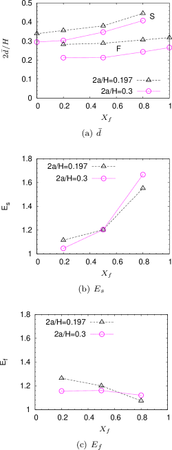
Figure 14: (color online) (a) Steady state $\bar{d}\;$as a function of $X_{f}$ for stiff and floppy particles at two different confinement ratios. Enrichment factor as a function of $X_{f}$ for (b) stiff particles, and (c) floppy particles.

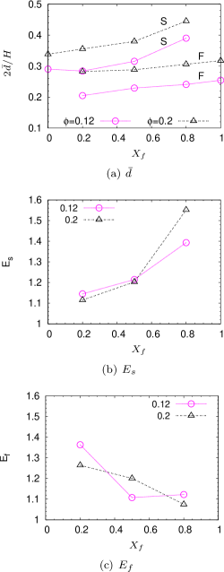
Figure 15: (color online) (a) Steady state $\bar{d}\;$as a function of $X_{f}$ for stiff and floppy particles at two different volume fractions. Enrichment factor as a function of $X_{f}$ for (b) stiff particles, and (c) floppy particles.

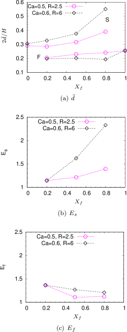
Figure 16: (color online) (a) Steady state $\bar{d}\;$as a function of $X_{f}$ for stiff and floppy particles as noted in the figure key. Enrichment factor as a function of $X_{f}$ for (b) stiff particles, and (c) floppy particles.

Appendix A Effect of confinement ratio, volume fraction and rigidity ratio

We present here some additional results of simulations with different confinement ratio, volume fraction or rigidity ratio than were used in the main text. The results are all consistent with those results and are included here for completeness.

To examine the effect of confinement ratio on the results, we consider suspensions with a volume fraction of $\phi=0.2$ and two different confinement ratios: $2a/H=0.197$ and $2a/H=0.3$. The rest of the parameters for these two simulation sets are listed in Tb (1) as sets A and B. We first show the effect of confinement ratio on $\bar{d}\;$for both the stiff and the floppy particles in Fig. (14a) as a function of $X_{f}$. As is obvious, $\bar{d}\;$of both the species decreases with increasing confinement ratio, i.e. an increasing fraction of the particles accumulate near the centerline with increasing $2a/H$. Moreover, the trend in $\bar{d}\;$of either species with varying $X_{f}$ is similar in both cases – with increasing fraction of floppy particles (increasing $X_{f}$), the stiffer particle gets increasingly displaced toward the wall, while with increasing fraction of stiffer particles (decreasing $X_{f}$), the floppy particles get increasingly displaced toward the centerline.

For a more quantitative measure of the segregation behavior, we compute the enrichment $E_{s}$ and $E_{f}$ of the two species as a function of $X_{f}$ (Figs. 14b, 14c). These plots show that $E_{s}$ increases more rapidly with $X_{f}$ in more confined suspension ($2a/H=0.3$), while $E_{f}$ increases more rapidly with decreasing $X_{f}$ in less confined suspension ($2a/H=0.197$). In other words, based on this measure, more confined suspensions lead to a higher maximum segregation of the stiff particles, while less confined suspensions leads to higher maximum segregation of floppy particles.

We now we briefly examine the effect of volume fraction on the segregation behavior in the suspension. Results will be reported here for a suspension with a volume fraction of $\phi=0.12$ and compared with the results of $\phi=0.2$ suspension discussed above in Sec. (III). The parameters for this simulation set are listed in Tb. (1) in the row labeled “C”, which are the same as in set A except for the volume fraction.

We begin by showing $\bar{d}\;$in Fig. (15a) for both the stiff ($\mathrm{Ca}=0.2$) and the floppy ($\mathrm{Ca}=0.5$) particles in the suspension as a function of $X_{f}$. For comparison, we also show $\bar{d}\;$for the $\phi=0.2$ suspension. At any given volume fraction, $\bar{d}\;$for stiffer particles is found to be higher than for floppy particles. Moreover, as the fraction of the floppy particles $X_{f}$ increases, $\bar{d}\;$for stiffer particles increases, i.e. they get increasingly displaced toward the wall. On the other hand, as the fraction of stiff particles in the suspension increases ($X_{f}$ decreases), $\bar{d}\;$for floppy particles decreases, i.e. they get displaced toward the centerline. All these trends in $\phi=0.12$ suspensions are similar to the trends in $\phi=0.2$ suspensions. It is also obvious in the plot that at any given value of $X_{f}$, the $\bar{d}\;$for a species increases with increasing $\phi$. This is an expected result, as at higher volume fractions the increased particle-particle interactions reduces the fraction of particles accumulating near the centerline, thereby leading to an increase in $\bar{d}\;$.

To quantify the degree of segregation, we compute the enrichment $E$ for both the species as a function of $X_{f}$ (Figs. 15b,15c). These plots confirm that the maximum enrichment of a given species is observed when that species is present in dilute amounts. Furthermore, the maximum enrichment of the stiff particles is higher for the $\phi=0.2$ suspension, while the maximum enrichment of floppy particles is higher for the $\phi=0.12$ suspension.

Finally, we consider the effect of $\mathrm{Ca}$ as well as that of the rigidity ratio $R$ on the segregation behavior. For this section, we compare the results of set C and set D in Tb. (1) – the volume fraction in both the simulations were $\phi=0.12$, while the stiff particles have a $\mathrm{Ca}$ of $0.2$ and $0.1$, and the floppy particles have a $\mathrm{Ca}$ of $0.5$ and $0.6$, respectively. These sets of $\mathrm{Ca}$ for the stiff and the floppy particles give a rigidity ratio of $R=2.5$ and $R=6$, respectively.

We begin by showing $\bar{d}\;$for both the stiff and floppy particles in these simulations in Fig. (16a). One can observe in the plot that $\bar{d}\;$for floppy particles is approximately the same in these two simulations. In contrast, $\bar{d}\;$for the stiffer particles in the two cases show a marked difference as a function of $X_{f}$ – at higher values of $R$, the stiffer particle gets increasingly displaced toward the walls as $X_{f}$ increases. For quantifying the degree of segregation between the two species, we again compute the enrichment factor $E$ for both the species as function of $X_{f}$ (Figs. 16b, 16c). As can be observed, $E_{s}$ shows a much larger increase with increasing $X_{f}$ for $R=6$ case in comparison to the $R=2.5$ case. In contrast, the enrichment of the floppy particles, $E_{f}$, is found to be nearly the same in both cases. These results suggest that the degree of segregation of the stiffer particle increases as the rigidity ratio increases, particularly at higher values of $X_{f}$.

References

- Tilles and Eckstein (1987) W. Tilles and E. C. Eckstein, Microvascular Research 33, 211 (1987).
- Jain and Munn (2009) A. Jain and L. L. Munn, PLos ONE 4, e7104 (2009).
- Suwanarusk et al. (2004) R. Suwanarusk, B. M. Cooke, A. M. Dondorp, K. Silamut, J. Sattabongkot, N. J. White, and R. Udomsangpetch, The Journal of Infectious Diseases 189, 190 (2004).
- Bunn (1997) H. F. Bunn, The New England Journal of Medicine 337, 762 (1997).
- Kaul et al. (1998) D. K. Kaul, X. Liu, R. L. Nagel, and H. L. Shear, The American Journal of Tropical Medicine and Hygiene 58, 240 (1998).
- Huang et al. (2010) R. B. Huang, S. Mocherla, M. J. Heslinga, P. Charoenphol, and O. Eniola-Adefeso, Molecular Membrane Biology 27, 312 (2010).
- Shevkoplyas et al. (2005) S. S. Shevkoplyas, T. Yoshida, L. L. Munn, and M. W. Bitensky, Analytical Chemistry 77, 933 (2005).
- Sethu et al. (2006) P. Sethu, A. Sin, and M. Toner, Lab Chip 6, 83 (2006).
- Hou et al. (2010) H. W. Hou, A. A. S. Bhagat, A. G. L. Chong, P. Mao, K. S. W. Tan, J. Han, and C. T. Lim, Lab Chip 10, 2605 (2010).
- Freund (2007) J. B. Freund, Physics of Fluids 19, 023301 (2007).
- Zhao and Shaqfeh (2011) H. Zhao and E. S. G. Shaqfeh, Physical Review E 83, 061924 (2011).
- Crowl and Fogelson (2011) L. Crowl and A. L. Fogelson, Journal of Fluid Mechanics 676, 348 (2011).
- Munn and Dupin (2008) L. L. Munn and M. M. Dupin, Annals of Biomedical Engineering 36, 534 (2008).
- Eckstein and Belgacem (1991) E. C. Eckstein and F. Belgacem, Biophysical Journal 60, 53 (1991).
- Pozrikidis (1992) C. Pozrikidis, Boundary Integral and Singularity Methods for Linearized Viscous Flow (Cambridge University Press, 1992).
- Kumar and Graham (2011) A. Kumar and M. D. Graham (2011), eprint arXiv:1109.6587, submitted for publication.
- Hernandez-Ortiz et al. (2007) J. P. Hernandez-Ortiz, J. J. de Pablo, and M. D. Graham, Physical Review Letters 98, 140602 (2007).
- Barthes-Biesel et al. (2002) D. Barthes-Biesel, A. Diaz, and E. Dhenin, Journal Of Fluid Mechanics 460, 211 (2002).
- Charrier et al. (1989) J. M. Charrier, S. Shrivastava, and R. Wu, Journal Of Strain Analysis For Engineering Design 24, 55 (1989).
- Pranay et al. (2010) P. Pranay, S. G. Anekal, J. P. Hernandez-Ortiz, and M. D. Graham, Physics of Fluids 22, 123103 (2010).
- Lac et al. (2007) E. Lac, A. Morel, and D. Barthès-Biesel, Journal of Fluid Mechanics 573, 149 (2007).
- Sherwood et al. (2003) J. Sherwood, F. Risso, F. Collé-Paillot, F. Edwards-Lévy, and M. C. Lévy, Journal of Colloid and Interface Science 263, 202 (2003).
- Zhao et al. (2010) H. Zhao, A. H. G. Isfahani, L. N. Olson, and J. B. Freund, Journal of Computational Physics 229, 3726 (2010).
- Meng and Higdon (2008) Q. Meng and J. J. L. Higdon, Journal of Rheology 52, 37 (2008).
- Kumar and Higdon (2010) A. Kumar and J. J. L. Higdon, Physical Review E 82, 051401 (2010).
- Doddi and Bagchi (2009) S. K. Doddi and P. Bagchi, Physical Review E 79, 046318 (2009).
- Phillips et al. (1992) R. J. Phillips, R. C. Armstrong, R. A. Brown, A. L. Graham, and J. R. Abbott, Physics Fluids A 4, 30 (1992).
- Nott and Brady (1994) P. R. Nott and J. F. Brady, Journal of Fluid Mechanics 275, 157 (1994).
- Li and Pozrikidis (2000) X. Li and C. Pozrikidis, International Journal of Multiphase Flow 26, 1247 (2000).
- Leal (1980) L. G. Leal, Annual Review of Fluid Mechanics 12, 435 (1980).
- Gardiner (2004) C. Gardiner, Handbook of Stochastic Methods: for Physics, Chemistry and the Natural Sciences (Springer-Verlag, 2004).
- Drazer et al. (2002) G. Drazer, J. Koplik, B. Khusid, and A. Acrivos, Journal of Fluid Mechanics 460, 307 (2002).
- Smart and Leighton (1991) J. R. Smart and D. T. Leighton, Physics of Fluids A 3, 21 (1991).
- Kumar and Higdon (2011) A. Kumar and J. J. L. Higdon, Journal of Rheology 55, 581 (2011).