Carbon $sp$ chains in graphene nanoholes

Abstract

Nowadays $sp$ carbon chains terminated by graphene or graphitic-like carbon are synthesized routinely in several nanotech labs. We propose an ab-initio study of such carbon-only materials, by computing their structure and stability, as well as their electronic, vibrational and magnetic properties. We adopt a fair compromise of microscopic realism with a certain level of idealization in the model configurations, and predict a number of properties susceptible to comparison with experiment.

1 Introduction

The carbon atom, with its three possible hybridization states, originates in nature very different elemental materials. The three possibilities ($sp^{3}$, $sp^{2}$, $sp$) correspond to three different prototypical structures: respectively diamond, graphitic-like structures (such as graphite, graphene, carbon nanotubes, and fullerenes), and linear carbon chains (known in the literature as polyynes [1, 2] or $sp$ carbon chains, spCCs in short).

spCCs were discovered in nature around 1968 [3], but their role in the arena of carbon-based nanostructures has been quite marginal: till very recently, spCCs have been considered as exotic allotropic forms, mainly present in extraterrestrial environments. Indeed, in the interstellar clouds formed in the explosions of carbon stars, novae, and supernovae, spCCs have been detected aside with fullerenes [4, 5], amorphous carbon dust, cyanopolyynes, and oligopolyynes. Indeed, in the phase diagram of carbon, the field of existence of spCCs coincides with that of fullerenes [6].

The high reactivity of spCCs [7], and their tendency to undergo cross-linking to form sp² structures, directed the experimental efforts towards complicate strategies for the stabilization of the spCCs with molecular end-groups or their isolation in inert matrices [1, 8, 9]. Thanks to novel synthetic routes and strategies [10], polyynes of increasing length and different type of termination have been successfully synthesized and characterized [11, 12, 13, 14, 15]. End-capped spCCs (often, but not exclusively, hydrogen-terminated) are being synthesized by chemical / electrochemical / photochemical methods [1, 16, 17, 18, 19]. spCCs have also been produced from carbon by dynamic pressure [17, 20]. spCCs or carbynoid material containing up to $300$ carbon atoms were synthesized, which opens a promising route toward molecular engineering of $sp$-carbon structures [16, 17, 21, 22].

Samples of pure carbon films grown by supersonic cluster beam deposition at room temperature have been characterized, and proven to contain a sizeable $sp$ component [23, 24]. These spCCs showed weaker stability relative to the $sp^{2}$ component upon exposition to low pressure gases at room temperature [25]. spCCs have also been produced from stretched nanotubes [26]. Recently, Jin et al. [27] have realized spCCs by stretching and thinning a graphene nanoribbon from its two free edges, by removing carbon rows until the number of rows becomes one or two. These spCCs show a good stability under the beam of a transmission electron microscope (TEM) for lengths up to a few nanometers. These experimental observations of spCCs formation during the controlled electron irradiation of graphene planes resulted in an rapidly increasing interest in this field [28, 29, 30, 31, 32, 33, 34, 35, 36].

Meanwhile, the existence of intrinsic magnetism in pure carbon has been a matter of debate for quite some time [37]. Possible effects due to magnetic contaminants on the experimental results have been discussed [38]. Subsequently, it has been shown that possible contamination effects are unable to explain quantitatively the measured ferromagnetism, supporting the idea that carbon magnetism has an intrinsic origin [39]. The existence of $\pi$-electron magnetism in pure carbon has now been widely accepted (see e.g. [40, 41]). On the theoretical side, it is well known that magnetic instabilities exist at specific graphene edges [42, 43, 44, 45], in defective graphene [46] and nanotubes [47].

The discovery of pure-carbon $\pi$-electron magnetism has also lead to speculations about possible applications of carbon-based magnetic materials in molecular electronic devices: for example, spintronic devices built around the phenomenon of spin-polarization localized at the 1-D zig-zag edges of graphene have been proposed [48]. Recently, the accent has been also put on the possibility to modify the magnetization optically [49]. Indeed, linear carbon chains are nowadays considered promising structures for nano-electronic applications [50, 51]. For example, they can be used as molecular bridges across graphene nanogap devices. Potential applications for the realization of non-volatile memories and two-terminal atomic-scale switches have been demonstrated [51].

The remarkable robustness of spCCs terminated on pure carbon, graphene-like fragments, combined with the fast progresses in the synthesis of graphene and graphene derivatives, could open the way towards the realization of actual nanodevices based on $sp$ + $sp^{2}$ carbon nanostructures. The interest of such systems stems from the possibility to exploit their peculiar semiconducting-magnetic behavior, in order to achieve novel characteristics and functions for the target devices.

Clearly, the possibility of designing graphene-based magnetic nanostructures is particularly intriguing. The capability of arranging the spins inside a carbon structure in a variety of ways, could open the way for the construction of completely novel devices [52]. Possible future applications for spCCs in interaction with the graphene-type system could be the construction of microchips with ferromagnetic or antiferromagnetic character that can be controlled by nanomanipulation and read out by nanocurrents.

In Sect. 2 we introduce the theoretical model, whose electronic structure we address by a standard ab-initio method based on the Density-Functional Theory (DFT). Section 3 presents the investigation of the structural and binding properties of a spCC inside a nanohole (nh) in a graphene sheet representing the $sp^{2}$ component in a carbon-only sample. Section 4 studies the magnetic properties of the nh edges and of the inserted spCCs. In Sections 5 and 6 we cover the band structures and selected vibrational properties of the studied nanostructures. In Sect. 7 we investigate the dynamical stability of the metastable spCC-nh structures, by means of a tight-binding molecular dynamics model. Section 8 discusses the results of simulations in the light of experimental data.

2 The model

In the present paper, we focus on spCCs bound to graphitic structures, represented by a hole in a infinite graphene sheet. This system is representative of a class of $sp+sp^{2}$ systems, which are at the core of an intense experimental work [23, 24, 25, 27, 28, 53, 54, 55]. To address the structural, vibrational, and electronic properties of spCCs inserted into a nanometer-sized hole defect of a graphene layer, we resort to the DFT. The plane-wave pseudopotential method and the Local Spin-Density Approximation (LSDA) to DFT have provided a simple framework whose accuracy have been demonstrated in a variety of systems [56]. The time-honored LDA is one in many functionals being used for current DFT studies of molecular and solid-state systems: other functionals often improve one or another of the systematic defects of LDA (underestimation of the energy gap, small overbinding and tiny overestimation of the vibrational frequencies), but to date no functional is universally accepted to provide systematically better accuracy than LDA for all properties of arbitrary systems. For a covalent system of $s$ and $p$ electrons as the one studied here, LDA is appropriate, and we expect our results to change by a few percent at most if the calculations were repeated using some other popular functional [57, 58, 59].

We compute the total adiabatic energies by means of the code Quantum Espresso [60], which computes forces by standard Hellmann-Feynman method. Each self-consistent electronic-structure calculation stops when the total energy changes by less than $10^{-8}$ Ry. We use ultrasoft pseudopotentials [61, 62], for which a moderate cutoff for the wave function/charge density of $30/240$ Ry is sufficient. We terminate atomic relaxation when all residual force components are smaller than $10^{-4}$ Ry$/a_{0}\simeq 0.04\,\mu$N.

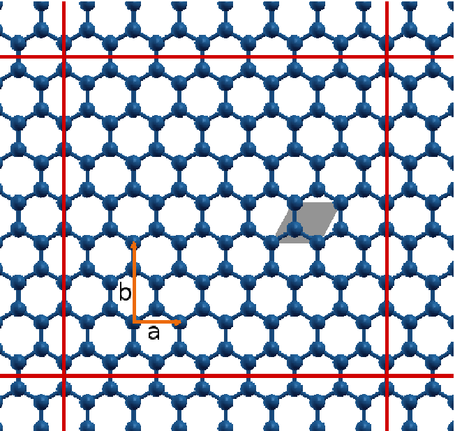
Figure 1: (Color online) The adopted slab model supercell for graphene, composed by $7\times 4$ conventional rectangular cells containing 4-atoms, each equivalent to two primitive unit cells of graphene (in gray). Solid: the unit vectors of the conventional cell, of length $a=244$ pm and $b=a\sqrt{3}\simeq 422$ pm. The size of the full supercell (delimited by the solid lines) in the $x-y$ plane is $1714$ pm $\times~{}1690$ pm.

Plane waves require periodic boundary conditions in all space directions. In our model, we represent a graphene plane in a $(x-y)$-periodically repeated $1714\times 1690$ pm² supercell consisting of $7\times 4$ rectangular conventional unit cells containing four carbon atoms each, see Fig. 1. Within this cell, a complete graphene layer is then represented by $112$ carbon atoms. We represent the graphite surface in the slab approximation, as one or a few stacked graphene layers: to ensure that the interaction between periodic images of the graphene sheet is negligible we interpose at least $1$ nm of vacuum along the $z$ direction. We have selected this cell size as it allows us to create reasonably large nanoholes in the graphene layers, with fairly small interaction between the supercell repeated copies of the nanohole itself, at the price of a manageable computer time. We cover electronic band dispersion the electron bands in the horizontal plane by means of a $5\times 5\times 1$ $\Gamma$-centered k-point mesh. BZ integration of the metallic band energies are performed using a $2\times 10^{-4}$ Ry-wide Gaussian smearing of the fermionic occupations.

2.1 The Nanohole

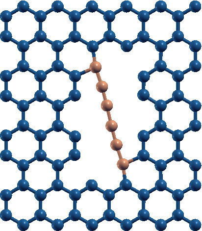
(a) Initial

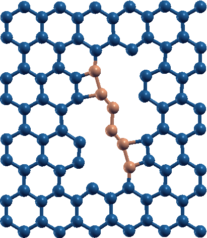
(b) Relaxed

Figure 2: (Color online) Initial and relaxed positions of a small nh with a C₆ polyyne: the lateral nh size is so small that no barrier prevents two polyyne atoms (brown/clear) to bind to the armchair edges.

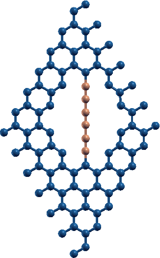
(a) Initial

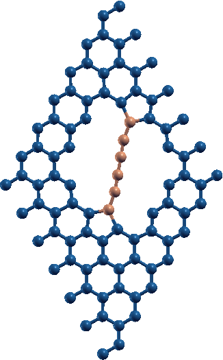
(b) Relaxed

Figure 3: (Color online) Initial and relaxed positions of a small nh with a C₆ polyyne: the lateral nh size is so small that no barrier prevents two polyyne atoms (brown/clear) to bind to the zig-zag edges and form pentagonal rings.

Starting from the perfect graphene foil of Fig. 1, we remove selected atoms in order to form a nh. The size of the nh should be such that inserted spCCs fit and only bind at their ends. If the nh is too small, then spCC atoms would tend to reconstruct the edges of the hole, as illustrated in the examples of Figs. 2 and 3. There, the small spCC-edge distance leads to spontaneous (barrier-free) edge reconstruction with the formation of additional squares or pentagons.

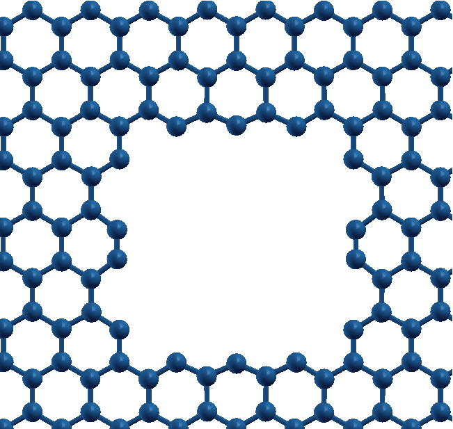
Figure 4: (Color online) A nh of sufficient size to lodge spCCs is obtained by removing $28$ atoms from the perfect graphene of Fig. 1. The rectangular hole has size $975$ pm $\times~{}985$ pm, and is delimited by both zig-zag and armchair edges

We must therefore construct a large enough nh, in particular allowing for a distance of at least $300$ pm between the spCC and the nearest nh edge in order to prevent recombination reactions. Figure 4 shows the minimal nh with such property. Starting from the perfect graphene of Fig. 1, the nh is obtained by removing $28$ atoms forming a rectangular hole of size $975$ pm $\times~{}985$ pm with both zig-zag armchair edges. The size of the nh permits us to investigate the insertion of several spCCs, from C₅ to C₈ atoms long, with various positions relative to the nh edges.

3 spCCs Binding to a Nanohole

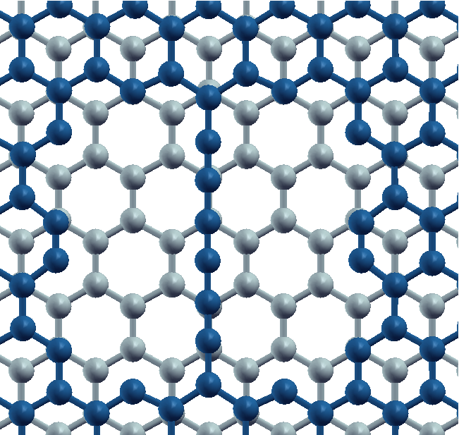
Figure 5: (Color online) A nano-indented graphite surface represented by a perfect graphene foil (pale gray) plus a superposed sheet with a nh (dark blue) as in Fig. 4 stacked in the standard AB arrangement of graphite. A C₆ chain (also dark blue) is connected to the zig-zag edge of the nh. The layer-layer distance equals $332$ pm.

In an experiment [23, 24, 25, 53], spCCs are likely to be bound to extended $sp^{2}$ structures, more reminiscent of graphite than of graphene. Such a configuration could be described for example with one layer of perfect graphene plus a layer with a nh, such as that described above Sect. 2.1. Figure 5 shows this configuration with the insertion of a C₆ polyyne. The upper graphene layer and the polyyne are fully relaxed, while the lower layer is kept frozen in ideal graphitic positions. The equilibrium distance between the two layers, $332$ pm, is very close to the observed interlayer distance of graphite, $335$ pm.

The resulting system composed of over $200$ atoms is computationally quite expensive: indeed, with a modern parallel computer using $32$ Xeon-class processors, it took more than two weeks to obtain a fully relaxed configuration. On the other hand, we verified that the properties of the upper layer do not change significantly without the lower (perfect) sheet, whose effective corrugation is quite small. Indeed, the forces between the two layers are weak long-range forces whose action is mild and almost translationally invariant, compared to the intra-layer forces acting in the nh layer. The DFT-LSDA evaluation of such weak dispersive forces is unreliable anyway. These observations suggest that it makes sense to consider the single layer containing the nh and the C_n spCC inserted into it, and leave the fixed substrate layer out. The relaxation of the positions, performed in the same conditions as above, took about one week only in this 1-layer configuration involving $90$ C atoms rather than 200 ones.

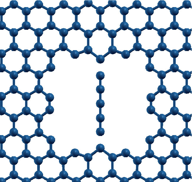
(a) nh-C₅

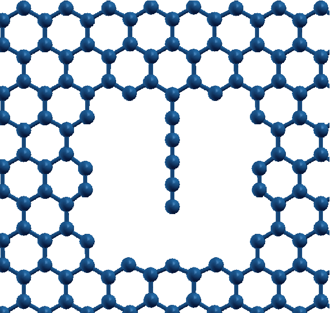
(b) nh-C₅ $1$b

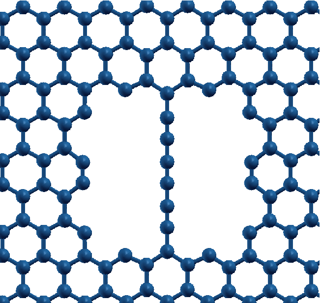
(c) nh-C₆ zig

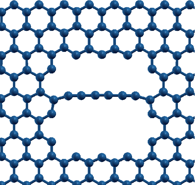
(d) nh-C₆ arm

(e) nh-C₇ straight, top view

(f) nh-C₈

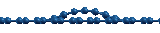
(g) nh-C₇ curved, side view

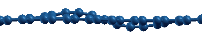
(h) nh-C₇ s-curved, side view

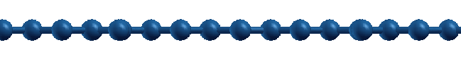
(i) nh-C₇ straight, side view

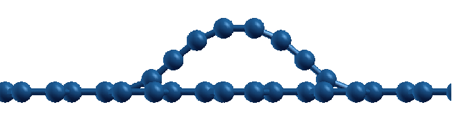
(j) nh-C₈ side view

                0.0                  0.5                  1.0                  1.5                     nm

Figure 6: (Color online) The relaxed configurations of the spCC-nanohole structures considered in the present paper and described in Table 1.

Label	Description	BLA	$E_{bond}$	$\sigma_{p}$	$\sigma_{v}$	$\sigma_{h}$
[Fig.]		[pm]	[eV]
nh-C5 [Fig. 6(a)]	A C5 chain stretched across the nh bonding weakly to both zig-zag edges (bond lengths: $170$ pm).	$7$	$\ 4.2$	✓	✓	✓
nh-C5 $1$b [Fig. 6(b)]	The C5 chain bonded to one zig-zag edge of the nh; all bond lengths of the spCC are similar to the lengths of cumulenic double bonds ($\simeq 127$ pm).	$1$	$\ 6.2$	✓	✓
nh-C6 zig [Fig. 6(c)]	A weakly stretched C6 chain bonded to the zig-zag nh edge.	$10$	$12.9$	✓	✓	✓
nh-C6 arm [Fig. 6(d)]	The C6 chain joining opposite armchair nh edges.	$12$	$\ 8.2$	✓	✓
nh-C7 curved [Fig. 6(g)]	A C7 connected to the zig-zag edges, and buckling out of the graphene plane (maximum spCC height $\simeq 120$ pm).	$3$	$12.0$		✓	✓
nh-C7 s-curved [Fig. 6(h)]	A C7 connected to the zig-zag edges, buckling in a s shape, with the central atom in the same plane as graphene.	$3$	$11.9$	*	✓	*
nh-C7 straight [Figs. 6(e), 6(i)]	A compressed straight C7 joining the zig-zag edges.	$2$	$11.8$	✓	✓	✓
nh-C8 [Figs. 6(f), 6(j)]	A C8 curved chain. The maximum height of the spCC equals $297$ pm.	$6$	$12.5$		✓	✓
wnh-$2$C6 [Fig. 7]	Two C6 spCCs inserted in a wider nh joining the zig-zag edges. The lateral distance between the spCCs equals $491$ pm.	$11$	n.c.	✓	✓	✓

Table 1: (Color online) Summary of the individual configurations considered for the spCCs bound to the nh. For the relaxed configurations we report the resulting BLA and total bonding energy $E_{bond}$, corresponding to the formation of the (usually two) bonds between the spCC and the nh. The relevant symmetry planes ($\sigma_{p}$ is the reflection across the graphene layer plane, $\sigma_{v}$ is the vertical plane through the spCC, $\sigma_{h}$ is the horizontal plane through the middle of the spCC) are marked for the configurations for which they apply.
^∗Individual $\sigma_{p}$ and $\sigma_{h}$ are not symmetries for nh-C₇ s-curved, but their product $\sigma_{p}\sigma_{h}$ is.

In our calculations, we consider several spCCs, from C₅ to C₈, placed in different positions inside the nh. We identify such compounds as nh-C_n, with further specification when different local minima are considered. Their relaxed configurations are depicted in Fig. 6. Table 1 summarizes the structural properties of the configurations considered, comparing in particular their bond-length alternation (BLA) [63] and the spCC-graphene bonding energy, defined as the total energy of the empty nh plus that of the isolated spCC minus the total energy of the bonded spCC-nh configuration under consideration.

For the selected nh size, C_n chains of different length can fit more or less easily inside the nh. Short chains such as C₅ or C₆ may fit at the price of a tensile stress, while longer spCCs can be forced inside the nh with a compressive strain, which could be eased by buckling [34, 64, 65].

Strain influences directly the spCC BLA: a tensile strain leads to stretching more the weaker bonds, thus producing an enhanced BLA, typical of polyynic spCC (in nh-C₆ arm, whose BLA reaches $12$ pm). Likewise, a BLA $\simeq 10$ pm is obtained for nh-C₆ zig due to the nh size being approximately $5\%$ larger than the equilibrium length of the spCC. In contrast, a compressive strain leads to a more cumulenic-type structure, e.g. nh-C₇ straight has BLA $\simeq 2$ pm. As was observed in a slightly different context [34], very small BLA variations are induced by lateral atomic displacements.

The linear size of the hole is approximately $95\%$ of the equilibrium length of the C₇ chain: different stable shapes of the spCC in nh-C₇ can be stabilized by the compressive strain [64]. We study three equilibrium geometries of the spCC: straight, single-curvature buckling, and s-curved buckling. The compressive strain depresses the BLA, so that for the three of them the BLA ranges from $2$ to $3$ pm.

The nh-C₅ is so much stretched that if kept in a central symmetric configuration bonding between the spCC and the two edges of the nh is weak, each highly stretched terminal bond contributing only about $\simeq-2$ eV to lowering the total energy. In such a condition we observe an intermediate BLA $\simeq 7$ pm. This configuration is locally stable, but if we displace the spCC significantly ($\simeq 50$ pm) closer to one nh edge than to the other, and then let it relax, we retrieve an energetically favored configuration (nh-C₅ $1$b) with essentially a single strong bond (total energy lowering: $\simeq-6$ eV) between the spCC and the nh. Here the spCC internal bond lengths are practically equal to those of isolated C₅.

Due to the small size of the nh, the C₈ chains can only fit in a curved geometry: the maximum out-of-plane elevation of the spCC equals $297$ pm. The resulting BLA $\simeq 6$ pm is intermediate between cumulenic and polyynic.

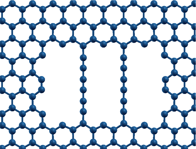
Figure 7: (Color online) Relaxed position of two C₆ spCCs in the wider nh: the hole width is 1504 pm, large enough to prevent the recombination of the two spCCs. This configuration displays no significant novelty relative to the single polyyne nh-C₆ zig configuration.

We also consider a wider nh in which one can insert more than one spCC: in wnh-$2$C₆, the nanohole contains two C₆ spCCs at a distance large enough to keep them separated, see Fig. 7. All properties are essentially equivalent to those of the nh-C₆ zig, therefore we will not further investigate this configuration.

We evaluate the bonding energy of the configurations described here. Due to its stretching, the nh-C₅ has a little value of $E_{bond}\simeq 4$ eV, while for the nh-C₅ $1$b $E_{bond}=6.2$ eV which can be considered a fair estimate of the spCC-graphene edge binding energy according to DFT-LSDA, and matches previous evaluations [25]. For all other configurations $E_{bond}\simeq 12$ eV indicative of the formation of two bonds, at the expense of approximately $1$ eV which accounts for the elastic deformation energy of the spCC and the connected graphene.

Until now the spCC was always connected to zig-zag edges. When a C₆ chain binds to the armchair edges (nh-C₆ arm), the bonding energy is smaller ($E_{bond}\simeq 9$ eV), due to the lower reactivity of the armchair edge relative to the zig-zag one [25, 66]. The BLA assumes a highly dimerized value $12$ pm associated to a tensile strain, like for the nh-C₆ zig isomer.

In the following we shall investigate the electronic properties of selected configurations. In particular, we first focus on the interplay of the magnetic behavior of the nh zig zag edges and of the spCC. We will then move on to describe the DFT-LSDA band structure, the vibrational properties, and the high-temperature stability of nh-C_n configurations.

4 Magnetism

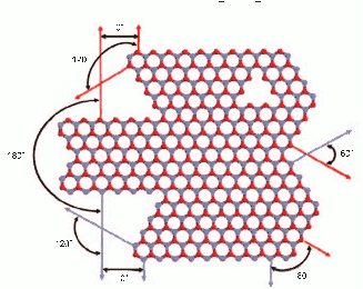
Figure 8: (Color online) Scheme of the geometric relation between adjacent graphene edges. The angle between edges is defined as the angle between the vectors normal to the edge. The edge atoms belong to the same sublattice (either dark/red or clear/gray) when the zig-zag edges are at a relative angle of $0^{\circ}$ or $120^{\circ}$; they instead belong to different sublattice when the relative angle is $60^{\circ}$ or $180^{\circ}$. (Adapted from Ref. [67].)

Zig-zag edges are generally known to be ferrimagnetic [44, 68] due to non-bonding localized edge states. A detailed investigation of the magnetic properties of graphene edge in the context of a nanohole was carried out by Yu et al. [67]. That work focused on zig-zag edges (armchair ones are known to be nonmagnetic [69]), which made it convenient to study diamond- or hexagon-shaped holes with zig-zag edges only. The main conclusion of Ref. [67] regarding consecutive zig-zag edges is that the relative alignment of magnetic moments tends to be ferromagnetic when the edge atoms belong to the same graphene sublattice. This conclusion can be rephrased in terms of the angle between the two consecutive edges, which is defined as the angle between the in-plane outward vectors normal to the edges, as illustrated schematically Fig. 8. Ferromagnetic correlations occur when subsequent zig-zag edges are unrotated ($0^{\circ}$) or rotated by $120^{\circ}$, as would happen in a triangular hole. In the opposite case, the magnetization is antiferromagnetic, as occurs for zig-zag edges rotated by $60^{\circ}$ or $180^{\circ}$ (relevant, e.g. for a diamond or and hexagonal hole).

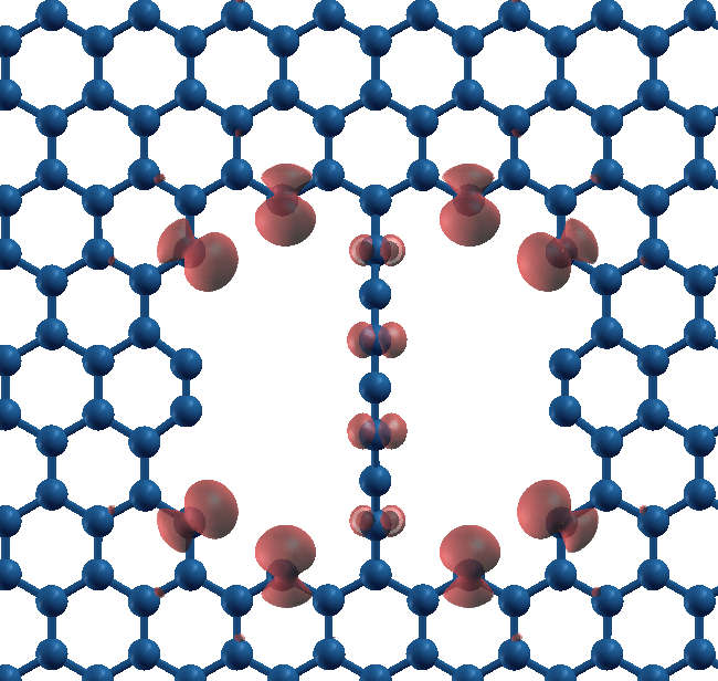
(a) nh-C₇

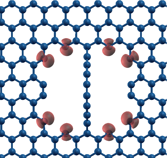
(b) nh-C₈

Figure 9: (Color online) The $0.01\,\mu_{\rm B}/a_{0}^{3}$ magnetic isosurface of the ferromagnetic state of nh-C₇ and of nh-C₈.

Our rectangular nh involves two armchair edges, which are long enough to isolate rather effectively the magnetic moments localized at the two zig-zag edges. In A, we study the magnetic properties of the edge of this nh. Following spCC insertion, all structures described in Sect. 3 preserve a nonzero absolute magnetization, associated to unpaired-spin electrons localized at the zig-zag nh edges. A significant magnetization is shared by the C_n spCCs with odd $n$, while the even-$n$ spCCs are non-magnetic, as illustrated by Fig. 9 for the nh-C₇ and nh-C₈ structures.

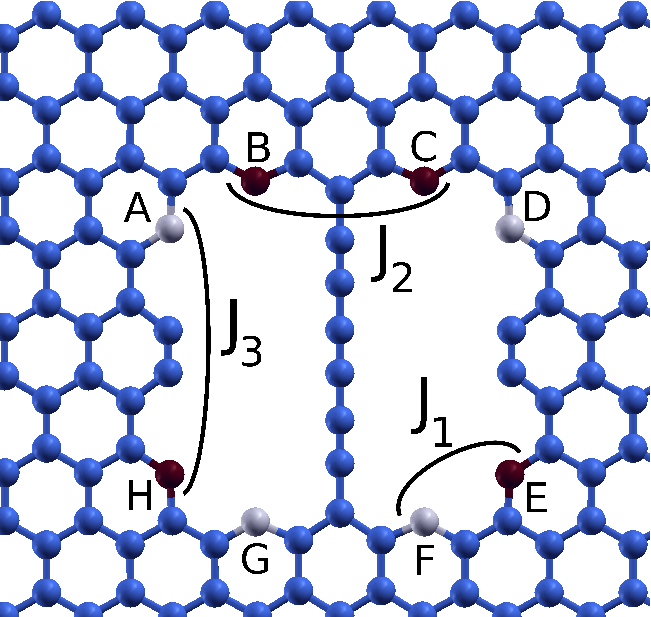
Figure 10: (Color online) To investigate nonferromagnetic structures we consider two fictitious atomic carbon species fixing the spin polarization at the initial stage of the self-consistent calculation. C_↑ (dark/red) and C_↓ (clear/gray) carry positive and negative initial magnetization, respectively. Arcs mark all symmetry-independent nearest-neighbor Ising-type magnetic couplings $J_{ij}$, see Eq. (1).

The ferromagnetic structures of Fig. 9 are induced by the choice of a uniform starting magnetization used to initialize the electronic self-consistent calculation. To investigate other possible magnetic arrangements, we need to start off the self-consistent calculation with different magnetic arrangements of the individual atoms. To do this, we define two fictitiously different atomic species, both with the same chemical nature of C, but with initial magnetizations of opposite sign ($\pm 1$ Bohr magneton). We place these initially magnetically polarized atoms along the zig-zag edges in order to trigger the desired magnetic structure. Figure 10 illustrates one of many possible arrangements of the C_↑ (dark/red) and C_↓ (clear/gray) atoms to initiate the self-consistent electronic-structure calculation.

4.1 C₆-nh

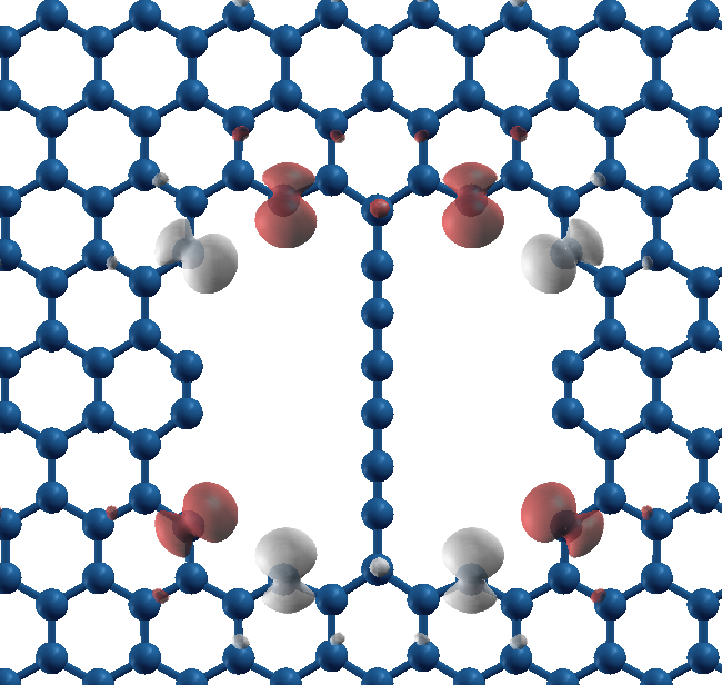
(a) Ground state: $E_{\rm tot}=$
$E_{\rm gs}=-13948.038$ eV
$M_{\rm tot}=0.00$
$M_{\rm abs}=9.31$

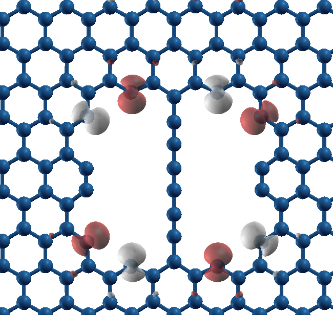
(b) $E_{\rm tot}=E_{\rm gs}+17$ meV
$M_{\rm tot}=0.00$
$M_{\rm abs}=8.21$

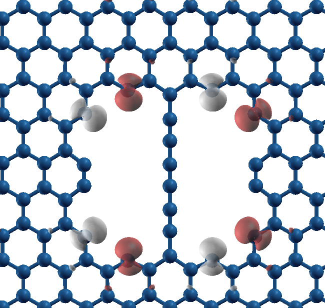
(c) $E_{\rm tot}=E_{\rm gs}+26$ meV
$M_{\rm tot}=0.00$
$M_{\rm abs}=8.03$

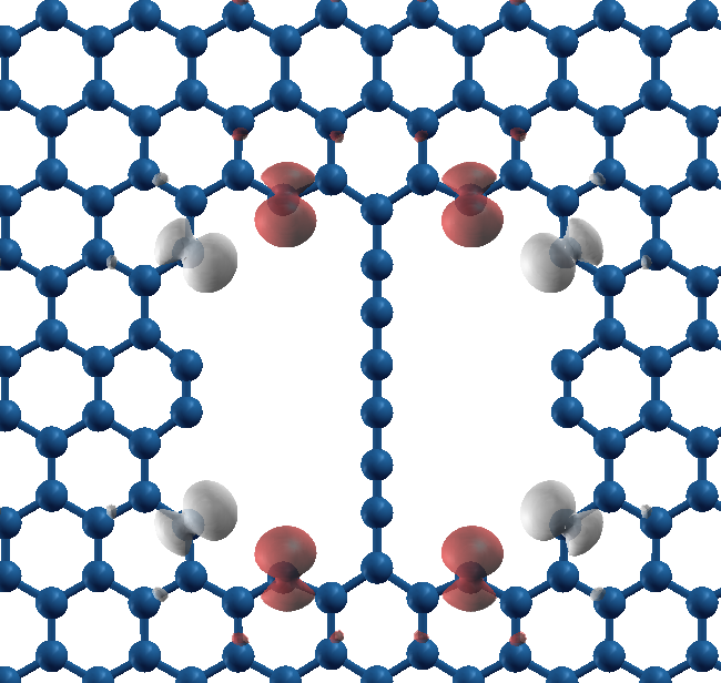
(d) $E_{\rm tot}=E_{\rm gs}+43$ meV
$M_{\rm tot}=0.00$
$M_{\rm abs}=8.38$

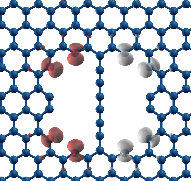
(e) $E_{\rm tot}=E_{\rm gs}+542$ meV
$M_{\rm tot}=0.00$
$M_{\rm abs}=8.67$

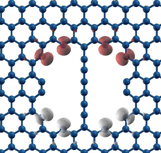
(f) $E_{\rm tot}=E_{\rm gs}+543$ meV
$M_{\rm tot}=0.00$
$M_{\rm abs}=9.19$

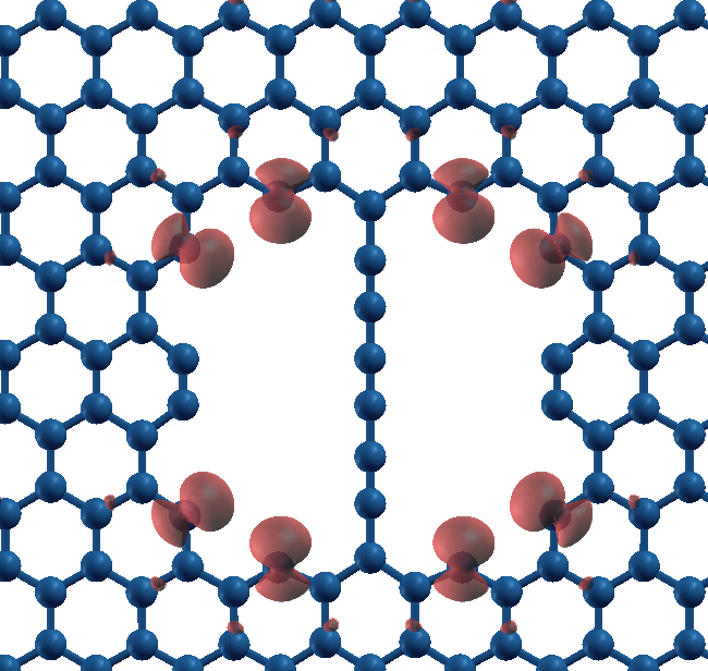
(g) $E_{\rm tot}=E_{\rm gs}+547$ meV
$M_{\rm tot}=8.00$
$M_{\rm abs}=8.66$

Figure 11: (Color online) Magnetization-density isosurfaces at $+0.01\,\mu_{\rm B}/a_{0}^{3}$ (dark/red) and $-0.01\,\mu_{\rm B}/a_{0}^{3}$ (clear/gray), for several different nh-C₆ magnetic structures. Frame (a): the DFT-LSDA ground state. Other frames: magnetically excited states. For each frame we report the relevant excitation energy, total magnetization and integrated absolute magnetization in Bohr magnetons $\mu_{\rm B}$.

We perform several self-consistent calculations for the nh-C₆ structure, considering different starting magnetizations, as shown in Fig. 11, and determine the ground magnetic configuration. In agreement with Ref. [67], the ground-state configuration, Fig. 11(a), has atoms of the the same magnetization in the same graphene sublattice (e.g. atoms labeled B, C, H, E in Fig. 10), and magnetization changes sign in passing from one sublattice to the other. The edge atoms bonded to even-$n$ C_n spCCs show little magnetism, mainly induced by the ferromagnetic interaction with neighboring atoms along the same zig-zag edge.

This ground-state magnetic configuration is relaxed completely, and the resulting total energy $E_{\rm gs}$ is taken as reference. Keeping fixed this fully relaxed ground atomic configuration, we repeat single self-consistent DFT-LSDA evaluations of the total energy, $E_{\rm tot}$, integrated magnetization $M_{\rm tot}=\int M_{z}(\vec{r})\,d^{3}\vec{r}$, and integrated absolute value of magnetization $M_{\rm abs}=\int|M_{z}(\vec{r})|\,d^{3}\vec{r}$, which we report next to each structure in Fig. 11. The resulting individual magnetic configurations, violating the opposite-sublattice rule, are low-lying excitations, which we obtain in the DFT-LSDA simulations by changing appropriately the initial magnetizations of selected atoms. Relaxation of one of these configurations shows very small displacements, not larger than 6 pm.

The excitation energies of such states can be described approximately within a Ising-model scheme. The $z$ component $S_{i}$ of the spin degree of freedom accounting for the magnetization at site $i$ interacts with neighboring spins $S_{j}$, with an energy

$$H_{\rm spin}=-\sum_{<i,j>}J_{ij}S_{i}S_{j}\,.$$ (1)

According to the values of the absolute magnetization reported in Fig. 11(a), it is appropriate to assume that each edge atom carries one Bohr magneton, i.e. one unpaired spin $1/2$, thus $S_{i}=\pm 1/2$. Accordingly, it makes sense to fit Ising-model energies only to configurations with an absolute magnetization significantly close to $8\,\mu_{\rm B}$. To avoid parameter proliferation, we neglect interactions between non-nearest-neighbor magnetic atoms.

Figure 10 identifies the $3$ independent Ising interaction parameters $J_{k}$ allowed by symmetry: $J_{1}$ for the interactions between unpaired spins in different sublattices on edges rotated by $60^{\circ}$ ($J_{1}=J_{AB}=J_{CD}=J_{EF}=J_{GH}$); $J_{2}$ for the interactions within the same zig-zag edge, but “isolated” by the spCC ($J_{2}=J_{BC}=J_{FG}$); and $J_{3}$ for the interactions across the armchair edge, representing opposite sublattices, or edges rotated by $180^{\circ}$ ($J_{3}=J_{AH}=J_{DE}$). We write the energy of a configuration as the sum of the magnetic energy $E_{\rm spin}$, approximated by the Ising expression (1), plus $E_{0}$, including covalency and all other interactions establishing the mean value of the total energy, averaged over all possible spin orientations. Specifically, for the nh-C₆ zig structure, we have:

$$E_{\rm spin}= - J_{1}\left(S_{A}S_{B}+S_{C}S_{D}+S_{E}S_{F}+S_{G}S_{H}\right)$$

$$- J_{2}\left(S_{B}S_{C}+S_{F}S_{G}\right)-J_{3}\left(S_{A}S_{H}+S_{D}S_{E}\right)\,,$$

so that, given the ground configuration of Fig. 11(a), we have $E_{\rm gs}=E_{0}+E_{\rm spin}=E_{0}+J_{1}+(J_{3}-J_{2})/2$.

Ising Parameter	Value [meV]	Standard deviation [meV]
$E_{0}-E_{\rm gs}$	$281$	$5$
$J_{1}$	$-259$	$5$
$J_{2}$	$-4$	$10$
$J_{3}$	$-17$	$10$

Table 2: (Color online) The interaction parameters of the Ising Model, Eq. (1), fitted on the DFT-LSDA values of the total energy of the magnetic configurations of nh-C₆ zig listed in Fig. 11.

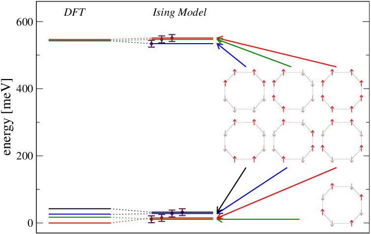
Figure 12: (Color online) Comparison of the DFT-LSDA energy levels of the magnetic structures of Fig. 11 (left) with the spectrum (right) obtained using the Ising model, based on parameteres fitting the DFT values.

We estimate the Ising-model parameters by means of a linear fit of the DFT energies with expression (4.1). Table 2 reports the best-fit values of $E_{0}$ and $J_{k}$: all the exchange energies $J_{k}$ turn out negative, reflecting antiferromagnetic interactions. The most significant value is $J_{1}$, reflecting the strong antiferromagnetic coupling of adjacent unpaired spins on edge atoms belonging to opposite sublattices. $J_{1}$ is over one order of magnitude greater than the weakly antiferromagnetic coupling $J_{3}$ across an armchair edge section. Given the fit standard deviation, the small value of $J_{2}$ is compatible with null coupling. The obtained small negative value is the result of a strong cancellation between the energy-order reversed configurations of panels 11(c), 11(d), and the regularly ordered states of panels 11(a), 11(b), the latter matching the ordering Ref. [67] as expected. Indeed the Ising-model ground state and first-excited level turn out almost degenerate and actually in reversed order due to the small positive value of $J_{2}$, as illustrated in Fig. 12.

In Fig. 12, we compare the energies of the different configurations of Fig. 11 obtained by DFT calculation with those obtained using the fitted Ising model. A remarkable feature of the DFT excitation spectrum is the tiny splitting of the levels of panels 11(e)-11(g), which is hardly compatible with a simple nearest-neighbor Ising model. Eventually Fig. 12 shows that the simple Ising model fails to describe the fine structure of the magnetic excitation of the edge atoms in the considered geometry. Only the significant $J_{1}$ energy, fixing the rough structure of the spectrum, is determined with fair accuracy. Of course one could easily modify the model to include e.g. second-neighbor interactions, to fit the detailed level structure, but that would take any predictive power out of the model.

4.2 C₇-nh

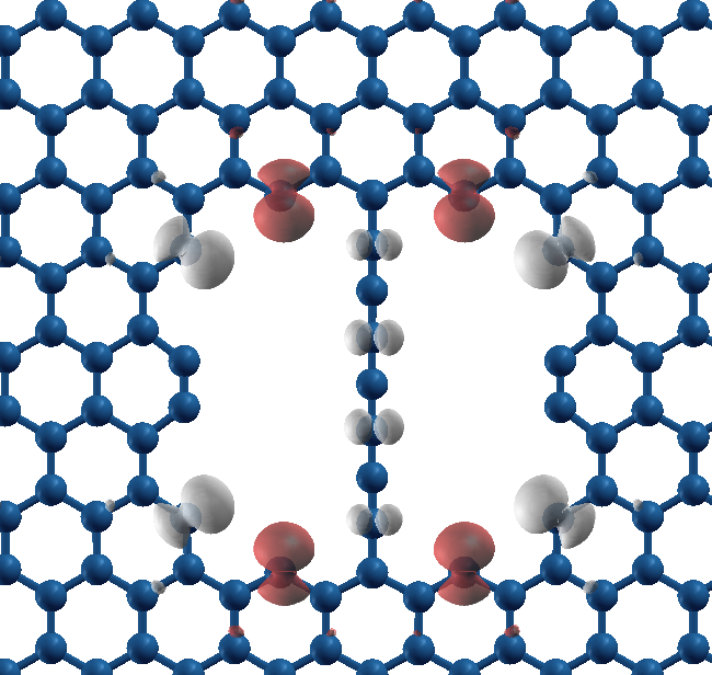
(a) Ground State
$E_{tot}=E_{\rm gs}=-14102.247$ eV
$M_{tot}=-0.80$
$M_{abs}=8.97$

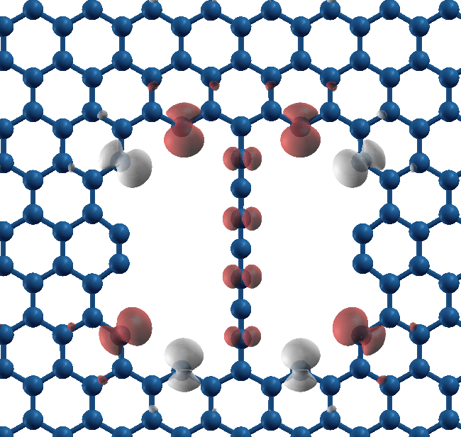
(b) $E_{tot}=E_{\rm gs}+60$ meV
$M_{tot}=-1.20$
$M_{abs}=9.63$

Figure 13: (Color online) Magnetization isosurfaces at $+0.01\,\mu_{B}/a_{0}^{3}$ (dark/red) and $-0.01\,\mu_{B}/a_{0}^{3}$ (clear gray) for two magnetic structures of nh-C₇ straight.

One may attempt a similar analysis for the odd-$n$ spCCs, e.g. nh-C₇. As Fig. 9(a) shows, odd-$n$ spCCs are magnetic, thus quite different from the even-$n$ ones. This leads to two consequences for odd spCCs attached to nh: first the spin values at different sites are different, and second the number of spin interactions to be considered is greater. This would leave little significance to a Ising model description.

It is possible to at least identify the ground magnetic configuration, like we did for even-$n$ chains. Figure 13 shows two different magnetic configuration of the nh-C₇ straight structure. The ground-state configuration is the one of Fig. 13(a), which follows the edge rules of Ref. [67]. The coupling between the spCC and nh edges is antiferromagnetic: this can be seen as a special case of the edge rules if the spCC atoms are seen as graphene atoms belonging to the edge but in the other sublattice relative to the outer zig-zag edge magnetic atoms. This coupling is so strong that it prevails over the weak antiferro long-range $J_{3}$-type coupling. One can estimate this magnetic coupling energy between the end spCC atom and one of the nearest zig-zag edge atoms to approximately $\approx 100$ meV. The intra-spCC interaction is distinctly antiferromagnetic.

5 Electronic Properties

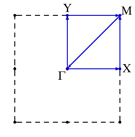
(a) k-point path

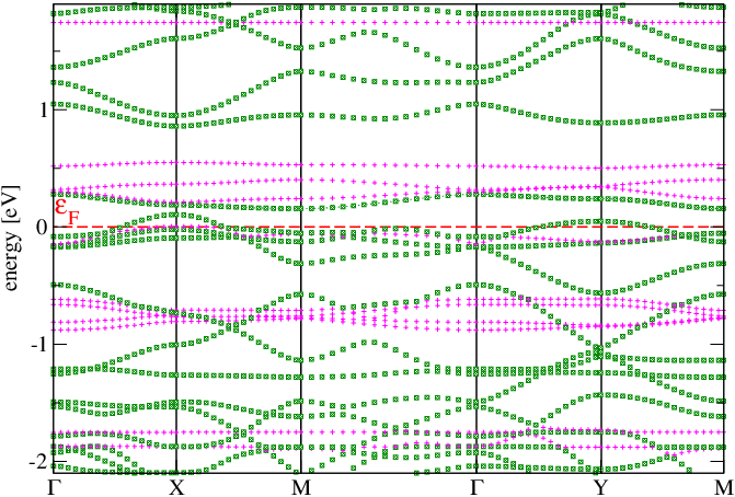
(b) nh bands

Figure 14: (Color online) (a): The Brillouin-zone (dashed) with the $\Gamma-X-M-\Gamma-Y-M$ k-point path adopted for all band-structure calculations of the present paper. (b) Spin-majority Kohn-Sham band structure of the relaxed nh superlattice of Fig. 4, in the ferromagnetic configuration of Fig. 26(f): magenta crosses stand for HE bands localized on the hole-edge; green squares represent delocalized BU states. The plot focuses a $4$ eV-wide energy region around the Fermi level (red dashed) for better readability.

The magnetic properties described in the previous section are determined by the electronic structure. Before analyzing the nanohole-spCC system, it is useful to examine the simpler bands of a empty nh. We will track the the bands along the Brillouin-zone path shown in Fig. 14(a). We sample the ${\bf k}$-space path with points separated by $1.75\times 10^{-13}$ m^-1.

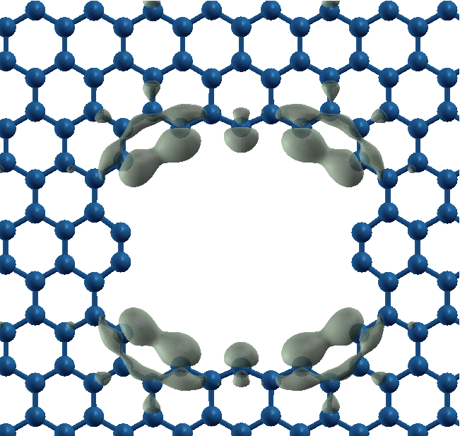
(a) A HE state

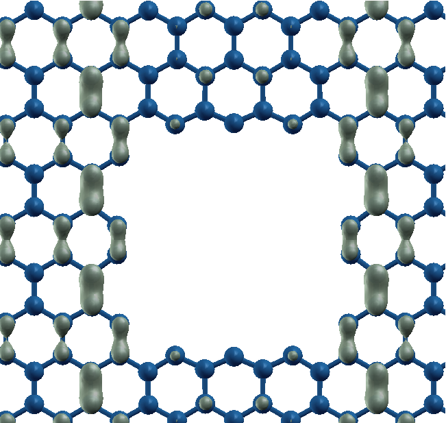
(b) A BU state

Figure 15: (Color online) Examples of ${\bf k}=0$ electronic states of the nh. (a): a localized HE state; (b): a BU state. In Fig. 14(b), these states are located at the $\Gamma$-point crossing at $-0.81$ eV and $1.36$ eV, respectively.

Figure 14(b) displays the band structure near the Fermi energy for the empty nh superlattice of Fig. 4. One can identify two kinds of bands, with different spatial localization properties of their wave functions: (i) States localized at the hole edge (HE), such as the one depicted in Figs. 15(a). We use magenta crosses to track these HE states in the bands-structure plots, such as Fig. 14(b). (ii) States like the one in Fig. 15(b) localized primarily on the bulk graphene atoms, with a weak component on the edge atoms. We label these states as BU, and identify them with green squares in band-structure plots.

HE bands are generally flat, with little dispersion. The small but nonzero bandwidth of HE states is due to the residual interaction between the nh and its periodic images. A HE band touches the Fermi energy near $X$, and is therefore only partly filled, thus becoming the responsible of the edge magnetism discussed in Sect. 4.

Liu et al. in their investigation of the band structures of a different graphene nanohole [70], discovered the opening of band gaps for nanoholes with either armchair or zig-zag edges. In contrast, our graphene with a isolated nh exhibits no band gap at the Fermi energy, and retains the (semi)metallic character of graphene. Specifically, a BU metallic band crosses $\epsilon_{F}$ and shows a modest but distinct dispersion, with sizeable empty hole pockets near the $X$ and $Y$ points.

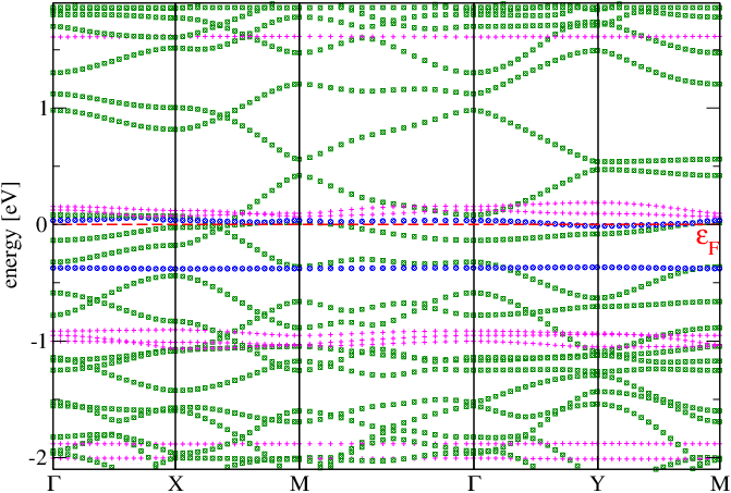
(a) nh-C₅

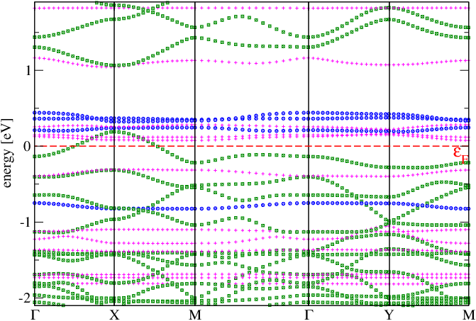
(b) nh-C₅ $1$b

Figure 16: (Color online) Spin-majority band structures of (a) nh-C₅, represented in Fig. 6(a), and of (b) nh-C₅ $1$b, Fig. 6(b).

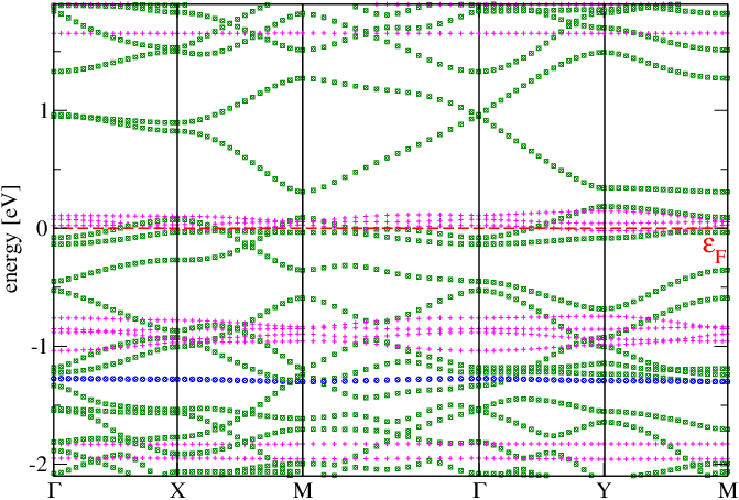
(a) nh-C₆ zig majority spin

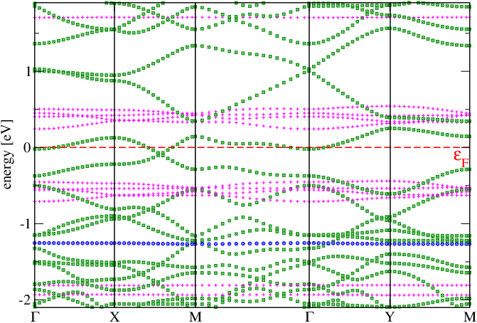
(b) nh-C₆ zig minority spin

Figure 17: (Color online) Band structure for the majority (a) and minority (b) spin components of the ferromagnetic state of nh-C₆ zig, depicted in Fig. 6(c).

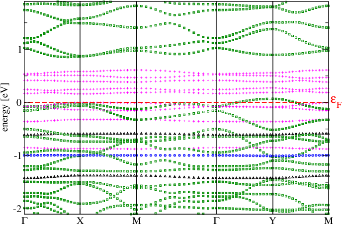
(a) nh-C₆ arm

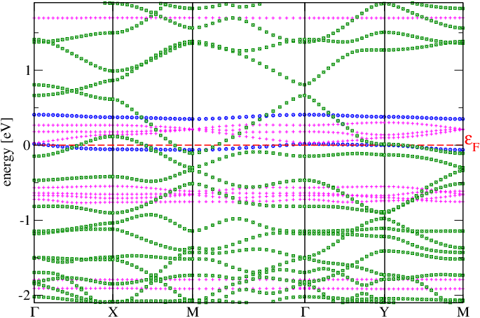
(b) nh-C₇

Figure 18: (Color online) Spin-majority band structures of (a) the nh-C₆ arm nanostructure, depicted in Fig. 6(d), and (b) nh-C₇, Fig. 6(e).

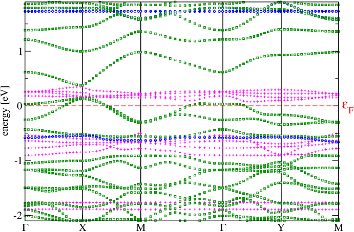
(a) nh-C₈

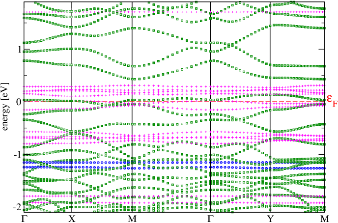
(b) nh-$2$C₆

Figure 19: (Color online) Spin-majority band structures of nh-C₈, see Fig. 6(f), and of nh-$2$C₆, see Fig. 7.

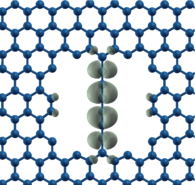
(a) A CB state

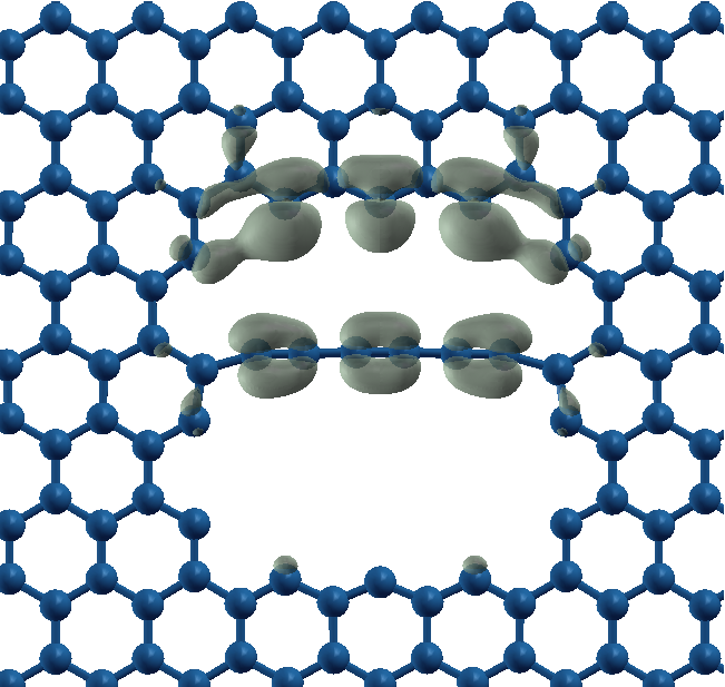
(b) A CHE state

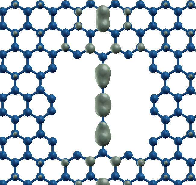
(c) A resonant bulk state

Figure 20: (Color online) Like in Fig. 15, but for nh-C₆ zig and nh-C₆ arm. (a): a typical CB state localized mainly on the polyyne – the $\Gamma$ state at energy $-1.16$ eV in Fig. 17(a); (b): a CHE state, localized jointly on the polyyne and the nh edge – the $\Gamma$ state at energy $-0.50$ eV in Fig. 18(a); (c): a bulk state showing a significant extension on the polyyne – the $\Gamma$ state at energy $-0.46$ eV in Fig. 17(a).

Coming to the nh-C_n systems, Figs. 16, 17, 18, and 19 report details of the computed DFT-LSDA bands for the relaxed structures of Figs. 6 and 7. Also in these band structures we identify HE (magenta crosses) and BU (green squares) bands. In addition, band states significantly localized on the spCC atoms (CB) are identified by blue circles. One such state is depicted in Fig. 20(a). Occasional resonances of localized spCC and nh-edge states lead to hybrid localized states involving both, e.g. the one of Fig. 20(b). We identify such “CHE” states only in nh-C₆ arm, and label them by black triangles in Fig. 18(a). Graphene bulk states often hybridize with the spCC molecular orbitals, thus acquiring a significant spCC components, as illustrated for example in Fig. 20(c). Our sample is too small to distinguish clearly between entirely localized states at the spCC/nh edge (whose bands would be perfectly flat in a realistically wide sample) and only partly localized hybrid states.

Essentially all structures display a metallic behavior, due to one or several bulk bands crossing the Fermi energy. The different bonded spCCs affect the graphene nh bands quite considerably, by both shifting them and deforming them especially near the Fermi energy. In particular, the positions of several localized states at the nh edge change depending on the spCC state, and moreover spCC-specific localized states occur. For even-$n$ spCCs, the CB states are energetically quite distant from the Fermi level, while odd-$n$ spCCs exhibit a more metallic behavior, with spCC states quite close to the Fermi energy, and significant hybridization with the extended bulk states, consistently with results of Ref. [25, 71].

The comparison of the spin majority and minority bands in Fig. 17 shows that magnetism affects the bulk bands only weakly. Magnetism appears to be associated to an energy shift of a few localized HE and (for odd spCCs) CB states near the Fermi level. The resulting effective exchange energy is $\simeq 0.3$ eV.

We perform several calculations of the nh-C₇ structure for each of the considered spCC shapes: curved – Fig. 6(g), s-curved – Fig. 6(h), and straight – Fig. 6(i). All these geometries show basically identical band structures, e.g. the one reported in Fig. 18(b). Likewise, no special effect of the spCC curvature is apparent in the bands of nh-C₈, Fig. 19(a). Finally, the congestion of the bands near the Fermi level in Fig. 19(b) is a consequence of the larger cell, and greater number of atoms and of electrons of this specific configuration. The general considerations (even-$n$ spCC bands away from the Fermi energy, magnetism related to HE bands near the Fermi energy) apply also in this more intricate configuration.

6 Vibrational spectra

We perform phonon calculation for a few stable structures of Sect. 3. We evaluate the phonon frequencies and eigenvectors of using standard density-functional perturbation theory, as implemented in the Quantum Espresso code [60, 72]. For comparison, the theoretical C-C stretching modes of polyynes C_nH₂ ($n=8-12$) evaluated with the same method match the experimental frequencies [73] to within 40 cm^-1. The size of the system is too large to evaluate the full dynamical matrix: although in principle possible, it would require a huge investment of computer time.

We focus specifically on spCC “optical” stretching modes, which are prominent and characteristic in the experimental spectra of $sp-sp^{2}$ carbon in the spectral region near 2000 cm^-1, while all other vibrations (the “acoustic” spCC stretching modes, all bending modes, all graphene vibrations) overlap and lump together in a continuum extending from 0 to 1600 cm^-1 [23, 25]. We verified that the spCC stretching modes are influenced very little by faraway ligand atoms [74]. Accordingly, we only compute and diagonalize the part of the dynamical matrix at $\Gamma$ relative to displacements of the atoms of the spCC, plus its first and second neighbors in the graphene sheet. The error in the vibrational frequency induced by this approximation can be estimated $\simeq 1$ cm^-1.

Structure name	Raman frequencies [cm-1]	IR frequencies [cm-1]
nh-C5	$1323$, $1368$	$1332$
nh-C6 zig	$1777$, $\mathbf{1878}$	$\mathbf{1939}$

Table 3: Wavenumber of Raman and IR spCC stretching frequencies calculated for the nh-C_n structures. The most intense Raman and IR frequencies are highlighted in bold.

By analyzing the displacement pattern of the normal modes of the even-$n$ spCCs, it is straightforward to identify the “$\alpha$” modes characterized by the strongest Raman and IR absorption [25, 54, 55, 75]. We take advantage of this pattern recognition to avoid a computationally expensive explicit evaluation of the Raman and IR intensities. Table 3 reports the computed frequencies of the spCC stretching modes, with the most intense Raman and IR mode highlighted. Note that the wavenumbers of the frequencies are significantly lower than the characteristic stretching-frequencies of free spCCs ($1950-2300~{}\rm{cm^{-1}}$). The reason is the tensile strain to which the spCCs are subjected by binding to the nh edges. In nh-C₅, the length of the chain, including the bonds between the spCC and the nanohole, is $15\%$ longer than the isolated spCC; this elongation leads to frequencies much softer than typical polyyne ones. The chain length in nh-C₆ zig is only $5\%$ longer than isolated length, and the frequencies come much closer to the typical frequencies of free spCCs.

The results of the present section do not imply that spCCs in a context of nanostructured $sp$-$sp^{2}$ carbon material should vibrate at much different frequencies from their molecular counterparts [54]. Quite on the contrary, previous calculations and experiments confirm that fully relaxed spCCs terminated by $sp^{2}$-type material exhibit very similar frequencies to those of molecular spCCs [25, 54, 55]. The results of the present calculations suggest instead that unrelaxed tensile strain in nanostructured $sp$ - $sp^{2}$ carbon material is likely to induce significant frequency shifts of the spCC modes. Depending on the method of production of spCC-containing material (e.g. cluster beam formation/deposition [23] vs. atomic wires stretched out from pulled graphene sheets [27, 28]), whenever a sizeable tensile strains remain frozen in the sample, one is to observe a corresponding distribution of the observed vibrational frequencies, quite independent of the frequency shifts associated to different lengths and terminations of the spCCs [55].

7 High-temperature stability

All studied configurations are local minima of the adiabatic potential energy, i.e. metastable allotropes of carbon. Given sufficiently long time, the spCCs are expected to degrade, for example by recombining with the nh edge and extend energetically favored $sp^{2}$ graphene. This possibility is however very remote at low temperature, because in this interconversion process the energy barriers to be crossed are quite substantial.

Since several detailed types of $sp\to sp^{2}$ processes are possible, a full study of the spCC degradation is beyond the scope of the present paper. We content ourselves with a semi-quantitative estimate of the thermal stability and the degradation mechanisms of spCCs bonded to carbon $sp^{2}$ nanostructures by running comparably long high-temperature molecular-dynamics (MD) simulations, and monitor the eventuality of spCC decomposition as a function of the simulated temperature.

As, due to the size dependency of statistical fluctuations, the longer the spCCs the higher is the chance of chain breaking. We therefore prefer to simulate a larger version of the model of Sect. 3, namely a C₁₀ chain bound to a nh large enough for it to fit loosely. Also the graphene plane is represented by four, rather than three hexagonal rings separating the nh periodic replicas. The resulting nh-C₁₀ structure involves 184 atoms and 736 electrons. Even using Car-Parrinello dynamics, it would be a formidable task to simulate several sufficiently long runs to expect a significant chance to observe spCC dissociation at a temperature comparable to experiment. For the present task therefore we abandon the ab-initio DFT-LSDA method for the treatment of the electronic degrees of freedom, and replace it with a tight-binding (TB) model [76]. We adopt the TB scheme of Xu et al. [77], which has been applied successfully to investigate several low-dimensional carbon systems [78, 79, 80, 81], as it reproduces well the experimental bulk equilibrium distance $d_{\rm graph}=1.4224$ Å of graphite, and the bulk structure and elastic properties of $sp^{3}$ diamond. Since all interatomic interactions vanish at a cutoff distance $r_{c}=2.6$ Å, which is shorter than the interlayer spacing of graphite, 3.35 Å [82], we focus on a single-layer model like we did for the DFT-LDA model above.

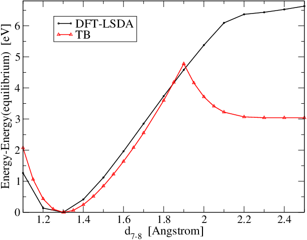
Figure 21: (Color online) Comparison of the total energy variation for a C₁₄ linear chain as a function of the (constrained) length $d_{7-8}$ of its central bond (between atoms 7 and 8), as obtained with DFT-LSDA and with TB.

To validate the TB force field for spCCs, we compute the total energy of a C₁₄ linear chain as a function of the length $d_{7-8}$ of its central bond (between atoms 7 and 8), which we keep fixed while all other bonds are allowed to relax. Figure 21 compares this total energy, referred to its value at full relaxation, as obtained with DFT-LSDA and with TB. The two models exhibit significant differences, in particular the TB model has a level crossing to a dissociative regime above 1.9 Å, while nothing of the sort occurs in the DFT-LDA band-structure calculation, which takes care of level degeneracies by selecting a spin-1 magnetic state. This problem with the TB model is characteristic of unsaturated conditions, while, in close-shell electronic configurations, dissociation is more regular. In general, the TB model is likely to be more “fragile” than a more realistic DFT-LDA. In turn the latter is also expected to be less strongly bounded than real spCCs, due to missing long-range attractive Van-der-Waals polarization correlation effects. We must then conclude that all quantitative stability evaluations based on the TB model are underestimates of the actual stability in experiment. Periodic boundary conditions (matching the zero-temperature lattice parameter of graphene) suppress long wavelength fluctuations, resulting in a stabilization of the thermal fluctuations, which in the thermodynamical limit would make the 1D - 2D structure unstable.

We run microcanonical (constant-energy) TB molecular dynamics (TBMD) simulations, since the temperature fluctuations are small enough ($\simeq 10\%$) in a sample of this size for temperature to be considered a fairly well defined quantity. The advantage of the microcanonical ensemble is that no thermostat artifacts, and in particular no dissipative term as in Langevin or Nosé-Hoover thermostats, can affect the atomic dynamics, allowing for a full account of local fluctuations to produce whatever bond breaking they may lead to. A disadvantage of the constant-energy MD is that, if a significant bonding breakdown of a part of the nanostructure occurs, the corresponding potential-energy increase occurs at the expense of the kinetic energy, thus the system may artificially cool down, thus hindering further decomposition. In practice, this problem has little importance for the system size considered. We use a time step of 0.5 fs, small enough to guarantee a rigorous global energy conservation within 0.02 eV, or 0.001%.

We run extended simulations of the model nh-C₁₀ structure at different temperatures, starting with a sampling of initial conditions. We generate starting configurations by beginning with the fully relaxed configuration and running three successive equilibration runs (0.1 ps, 0.1 ps and 0.5 ps), with randomized initial velocities, taken from a Gaussian distribution matching the Boltzmann distribution at the target temperature. In the figures we indicate the resulting temperature, with an error bar appropriate to the determination of the average along the whole simulation, (thus not estimating the instantaneous temperature fluctuations, which are much larger). In the determination of this average temperature, we drop the first 100 fs, to minimize the systematic oscillations induced by starting with initial random velocities with little correlation to the forces.

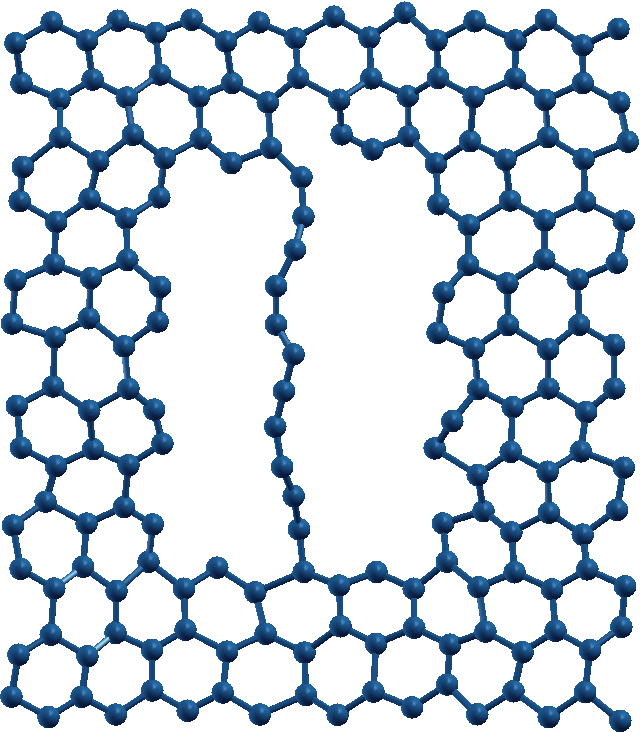
(a) $t=0$ ps

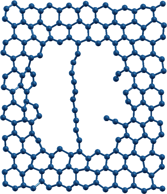
(b) $t=1.5$ ps

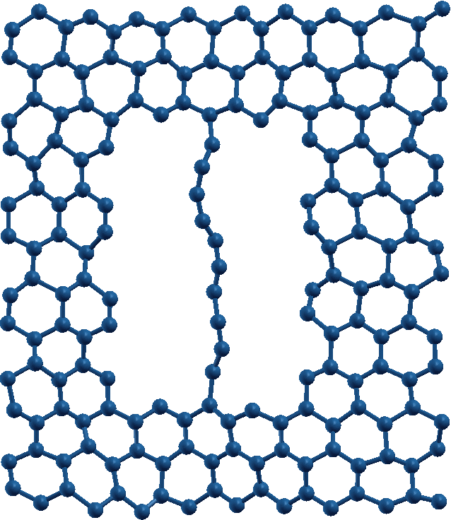
(c) $t=2.5$ ps

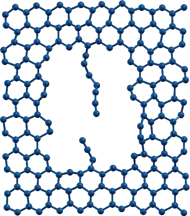
(d) $t=2.7$ ps

Figure 22: (Color online) Successive snapshots of a sample TBMD simulation at a temperature $T=(3991\pm 10)$ K of nh-C₁₀.

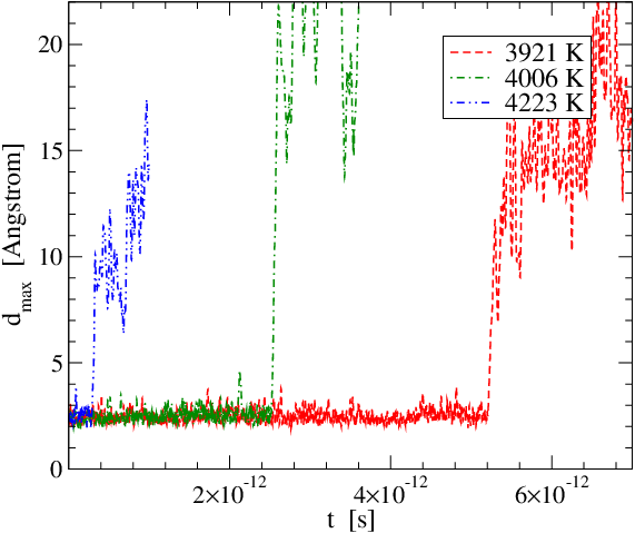
Figure 23: (Color online) The time dependence of the longest bond length $d_{\rm max}$, Eq. (3), of the C₁₀ chain in four simulations at different temperature.

Figure 22 displays successive frames of an example simulation illustrating that edge reconstruction processes – Fig. 22(b) – often occur before the earliest spCC breakdown event – Fig. 22(d). To monitor these breakdown events, a clear indicator is the longest C-C bond length relative to the 11 bonds of the C₁₀ chain and of the chain ends to the attached nh edge atoms:

$$d_{\rm max}=\max_{i=0,1,..10}d_{\rm C_{i}-C_{i+1}}\,.$$ (3)

Figure 23 reports the time dependency of $d_{\rm max}$ following 4 independent simulations carried out at different temperature, with different initial states. Chain breakdown, as happens between frames 22(c) and 22(d), is signaled by the rapid increase of one of the bond lengths beyond $5$ Å. The spCC breakdown may be followed by recombination of the chain into the nh edge, or even expulsion of a section of the spCC into vacuum.

As suggested by Fig. 23, spCC breakdown occurs, on average, earlier and earlier for increasing temperature. By repeating the numerical simulations for different initial conditions but similar temperature we estimate an average decay rate by averaging the inverse times before decay. The average decomposition rate time $\bar{k}$ is an increasing function of temperature. In simulations done at substantially lower temperature than the ones considered in Fig. 23, one would need to wait too long to observe decomposition, while at much higher temperature decomposition occurs immediately after start.

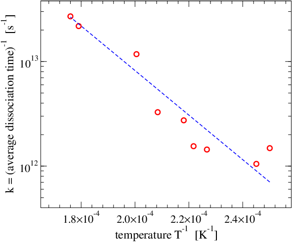
Figure 24: (Color online) Circles: the average inverse time before the breakdown of the C₁₀ spCC, as a function of inverse temperature. Dashed line: a Arrhenius fit, Eq. (4).

If one can assume that one type of process (bond breaking) dominates over all decomposition channels, the decomposition rate ${\bar{k}}$ is expected to be in the Arrhenius form

$${\bar{k}}=A\exp\left(-\frac{E_{a}}{k_{\rm B}T}\right)\,.$$ (4)

We estimate the attempt frequency $A$ and the effective energy barrier $E_{a}$ of the TBMD model by fitting the Arrhenius plot in Fig. 24. The value $E_{a}=4.2$ eV matches the TB breakup of Fig. 21: this effective activation barrier is surely an underestimation of the actual barrier against breakup. The estimated attempt rate $A=1.5\times 10^{17}$ s^-1, although probably slightly overestimated, reflects the high number of breakup channels available for decomposition of the spCC [83]. If we assume the computed values for $E_{a}$ and $A$, we extrapolate thermal decay rates of spCCs in $sp^{2}$ carbon of the order of ${\bar{k}}=7.5\times 10^{-5}$ s^-1 at 1000 K, and ${\bar{k}}=1.5\times 10^{-54}$ s^-1 at room-temperature (300 K). Overall, the calculations of the present section confirm a substantial stability of spCCs in the solid state and in vacuum. In the lab, whenever $sp-sp^{2}$ carbon is not kept in vacuum, chemical decay mechanisms are therefore likely to overcome the thermal ones.

8 Discussion and conclusion

The present work collects extensive investigation of the geometry, electronic structure, magnetic properties, and dynamical stability of spCCs attached to $sp^{2}$ graphitic fragments. When a spCC binds to zig-zag graphene edges, its polyynic character is attenuated to a value intermediate between those typical of cumulenes and polyynes. The attachment of a spCC to the graphene edge is very stable: we predict stabilization energies near $6$ eV per bond between each chain end and the $sp^{2}$ regions. Thermal excitations typically break bonds along the spCC with similar probability to those formed with the graphene edge, which indicates a very solid attachment.

Odd spCCs in the nh display a metallic behavior, with at least one band pinned to the Fermi energy, while even spCCs have little overlap with the states at the Fermi level [50, 51, 84, 85]. The partly filled states of odd-$n$ spCCs are associated to nonzero magnetization related to a spin triplet state of the $\pi$ bonds. Even-$n$ spCCs are instead insulating and non-magnetic, and in this context only the magnetic moments of the graphene edge contribute to the magnetism of the nh-C_2m structures, and only the bulk graphene states provide conducting bands.

We compute also the vibrational modes, and specifically the optical C$\equiv$C stretching modes which emerge as a characteristic signature of spCCs in Raman and IR spectroscopies. Our calculations show that the vibrational frequencies can be quite substantially red-shifted when spCCs are kept under tensile stress. Indeed, the weaker stability and correspondingly faster decomposition rate of strained spCCs is likely to play a significant role in the overall blue shift of the $sp$-carbon peak in the Raman spectrum of the decaying spCCs in cluster-assembled $sp$-$sp^{2}$ film [25].

Appendix A Magnetism at the edge of the empty nh

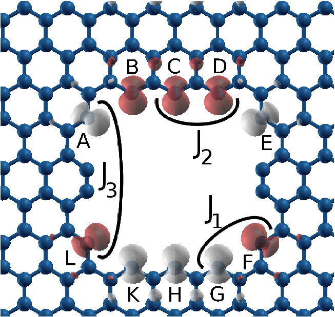
Figure 25: (Color online) Magnetization-density isosurfaces at $+0.01\,\mu_{B}/a_{0}^{3}$ (dark/red) and $-0.01\,\mu_{B}/a_{0}^{3}$ (clear gray) for the magnetic ground state of the unpaired-spin electrons localized at the zig-zag edges of the empty nh. Letters label the spin-carrying atomic sites. Arcs mark all symmetry-independent nearest-neighbor Ising-type magnetic couplings $J_{i}$, see Eq. (1).

As magnetism is intrinsic of the zig-zag graphene edge, thus even a empty nanohole exhibits a range of magnetic states similar to those arising in the presence of even-$n$ spCCs. The zig-zag edge atoms involved in magnetism are clearly identified in Fig. 25. Also here, each atomic site A–L carries a magnetization close to $1\,\mu_{\rm B}$. As illustrated in Fig. 25, even though the number of spin-carrying atoms is larger than in the case of Sect. 4.1, only three independent nearest-neighbor interactions need to be considered. Two of them, $J_{1}$ and $J_{3}$, represent interaction between two edges belonging to different sublattices (where we expect an anti-ferromagnetic character). In contrast, the coupling $J_{2}$ accounts for the interaction of spins within the same edge, and is therefore expected to be ferromagnetic, according to Ref. [67].

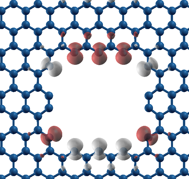
(a) Ground State
$E_{\rm tot}=E_{\rm gs}=-13017.539$ eV
$M_{\rm tot}=0.00$
$M_{\rm abs}=11.76$

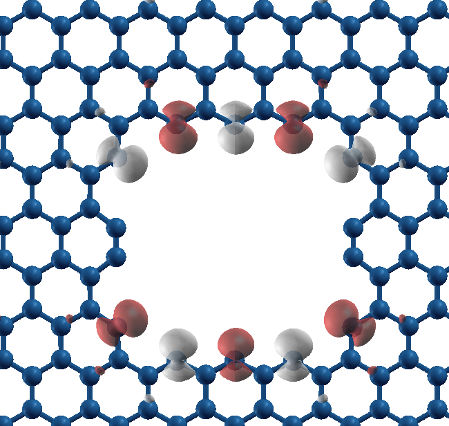
(b) $E_{\rm tot}=E_{\rm gs}+52$ meV
$M_{\rm tot}=0.00$
$M_{\rm abs}=10.05$

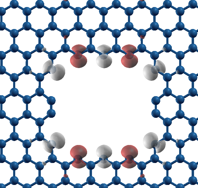
(c) $E_{\rm tot}=E_{\rm gs}+72$ meV
$M_{\rm tot}=-2.00$
$M_{\rm abs}=9.71$

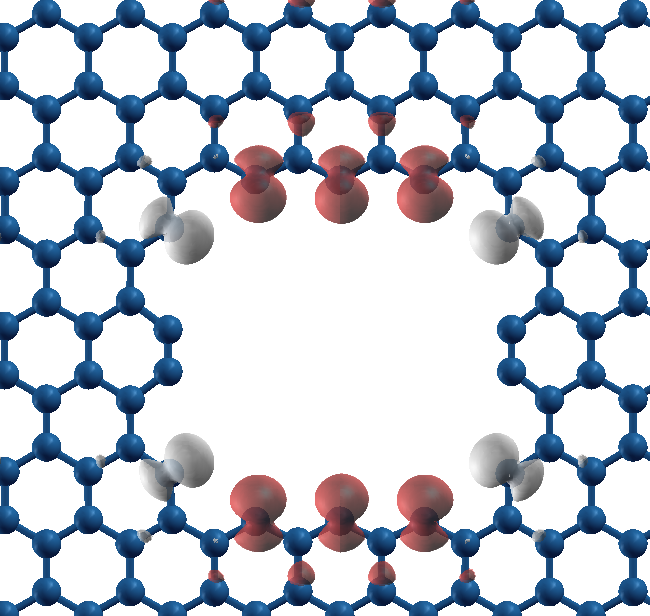
(d) $E_{\rm tot}=E_{\rm gs}+86$ meV
$M_{\rm tot}=2.00$
$M_{\rm abs}=10.77$

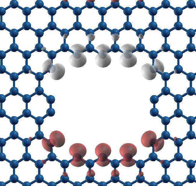
(e) $E_{\rm tot}=E_{\rm gs}+513$ meV
$M_{\rm tot}=0.00$
$M_{\rm abs}=11.52$

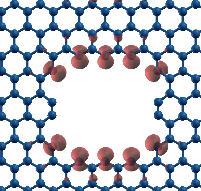
(f) $E_{\rm tot}=E_{\rm gs}+565$ meV
$M_{\rm tot}=10.00$
$M_{\rm abs}=10.77$

Figure 26: (Color online) Magnetic positive (dark/red) $+0.01\,\mu_{\rm B}/a_{0}^{3}$ and negative (clear/gray) $-0.01\,\mu_{\rm B}/a_{0}^{3}$ isosurfaces for the empty nanohole structures.

Ising Parameter	Value [meV]	Standard deviation [meV]
$E_{0}-E_{\rm gs}$	$300$	$12$
$J_{1}$	$-248$	$12$
$J_{2}$	$10$	$12$
$J_{3}$	$-53$	$19$

Table 4: (Color online) The individual Ising-model parameters computed for the nh magnetic configurations.

As done in Sect. 4.1 for the nh-C₆ structures, we make a linear fit of all considered magnetic configurations (shown in Fig. 26), to evaluate the values of the $J_{i}$ and of $E_{0}$. In the Ising model, the total energy is written as:

$$E_{\rm tot}=E_{0}+E_{\rm spin}=E_{0} - J_{1}\left(S_{A}S_{B}+S_{D}S_{E}+S_{F}S_{G}+S_{K}S_{L}\right)+$$ (5)

$$- J_{2}\left(S_{B}S_{C}+S_{C}S_{D}+S_{G}S_{H}+S_{H}S_{K}\right)+$$

$$- J_{3}\left(S_{A}S_{L}+S_{E}S_{F}\right)\,.$$

The result of the linear fit of the energies of the magnetic configurations of Fig. 26 is reported in Table 4. Like in nh-C₆, $J_{1}$ is much larger than the other antiferromagnetic coupling $J_{3}$. Indeed, the $J_{1}$ interaction is very similar to the one obtained in the calculations with the nh-C₆ structure, see Table 2. Moreover, like in the nh-C₆ case, given the relevant error bar the weakly ferromagnetic $J_{2}$ is in fact compatible with a null value, which is somewhat surprising for neighboring atoms along the same zig-zag edge.

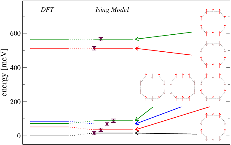
Figure 27: (Color online) A comparison of the DFT-LSDA magnetic energy levels of the structures of Fig. 26, with those obtained based on the Ising model, Eq. (5), fitted on the DFT-LSDA energies for the empty nh.

Figure 27 compares the DFT-LSDA energy levels and those obtained using the fitted Ising model. Here the fit agrees better than in the nh-C₆ case, but clearly the role of the $J_{2}$ coupling is contradictory, which explains its small value.

References

References

- [1] Polyynes: Synthesis, Properties, and Applications, edited by F. Cataldo (CRC, Taylor&Francis, London, 2005).
- [2] Since “polyyne” indicates an alternating single-triple-bond carbon chain, we use the more generic “ carbon chain” to include also undimerized species, such as cumulenes or odd- Cn chains.
- [3] A. El Goresy and G. Donnay, Science 161, 363 (1968).
- [4] H. Kroto, Carbon 30, 1139 (1992).
- [5] W. W. Duley, and A. Hu, Astrophys. J. 698, 808 (2009).
- [6] F. P. Bundy, W. A. Bassett, M. S. Weathers, R. J. Hemley, H. K. Mao, and A. F. Goncharov, Carbon 34, 141 (1996).
- [7] R. H. Baughman, Science 312, 1009 (2006).
- [8] H. Matsuda, H. Nakanishi, and M. Kato, J. Polym. Lett. Ed. 22, 107 (1984).
- [9] Y. P. Kudryavtsev, Progress of Polymer Chemistry, 87, Nauka (Moscow, 1969).
- [10] F. Cataldo, D. Capitani, Materials Chem. Phys. 59, 225 (1999).
- [11] W. Mohr, J. Stahl, F. Hampel, and J. A. Gladysz, Chem. Eur. J. 9, 3324 (2003).
- [12] X. Zhao, Y. Ando, Y. Liu, M. Jinno, and T. Suzuki, Phys. Rev. Lett. 90, 187401 (2003).
- [13] Y. Liu et al., Phys. Rev. B 68, 125413 (2003).
- [14] K. Inoue, R. Matsutani, T. Sanada, and K. Kojima, Carbon 48, 4209 (2010).
- [15] C. A. Rice, V. Rudnev, R. Dietsche, and J. P. Maier, Astron. J. 140, 203 (2010).
- [16] M. Kijima, T. Toyabe, and H. Shirakawa, Chem. Commun. 19, 2273 (1996).
- [17] R. B. Heimann, S. E. Evsyukov, and L. Kavan, Carbyne and Carbynoid Structures (Kluwer, Dordrecht, 1999).
- [18] M. Tsuji, S. Kuboyama, T. Matsuzaki, and T. Tsuji, Carbon 41, 2141 (2003).
- [19] F. Cataldo, Tetrahedron Lett. 45, 141 (2004).
- [20] K. Yamada, H. Kunishige, and A. B. Sawaoka, Naturwiss 78, 450 (1991).
- [21] K. Ohmura, M. Kijima, and H. Shirakawa, Synth. Metals 84, 417 (1997).
- [22] M. Kijima, Recent Res. Devel. Pure Appl. Chem. 1, 27 (1997).
- [23] L. Ravagnan, F. Siviero, C. Lenardi, P. Piseri, E. Barborini, and P. Milani, Phys. Rev. Lett. 89, 285506 (2002).
- [24] L. Ravagnan, P. Piseri, M. Bruzzi, S. Miglio, G. Bongiorno, A. Baserga, C. S. Casari, A. Li Bassi, C. Lenardi, Y. Yamaguchi, T. Wakabayashi, C. E. Bottani, and P. Milani, Phys. Rev. Lett. 98, 216103 (2007).
- [25] L. Ravagnan, N. Manini, E. Cinquanta, G. Onida, D. Sangalli, C. Motta, M. Devetta, A. Bordoni, P. Piseri, and P. Milani, Phys. Rev. Lett. 102, 245502 (2009).
- [26] H. E. Troiani, M. Miki-Yoshida, G. A. Camacho-Bragado, M. A. L. Marques, A. Rubio, J. A. Ascencio, and M. Jose-Yacaman, Nano Lett. 3, 751 (2003).
- [27] C. Jin, H. Lan, L. Peng, K. Suenaga, and S. Iijima, Phys. Rev. Lett. 102, 205501 (2009).
- [28] A. Chuvilin, J. C. Meyer, G. Algara-Siller, and U. Kaiser, New J. Phys. 11, 083019 (2009).
- [29] I. M. Mikhailovskij, E. V. Sadanov, T. I. Mazilova, V. A. Ksenofontov, and O. A. Velicodnaja, Phys. Rev. B 80, 165404 (2009).
- [30] M. G. Zeng, L. Shen, Y. Q. Cai, Z. D. Sha, and Y. P. Feng, Appl. Phys. Lett. 96, 042104 (2010).
- [31] W. A. Chalifoux and R. R. Tykwinski, C. R. Chimie 12, 341 (2009).
- [32] E. Hobi Jr., R. B. Pontes, A. Fazzio, and A. J. R. da Silva, Phys. Rev. B 81, 201406 (2010).
- [33] B. Akdim and R. Pachter, ACSNano 5, 1769 (2011).
- [34] Y. H. Hu, J. Phys. Chem. C 115, 1843 (2011).
- [35] L. Ravagnan, T. Mazza; G. Bongiorno, M. Devetta, M. Amati, P. Milani, P. Piseri, M. Coreno, C. Lenardi, F. Evangelista and P. Rudolf, Chem. Commun. 47, 2952 (2011).
- [36] E. Erdogan1, I. Popov, C. G. Rocha, G. Cuniberti, S. Roche, and G. Seifert, Phys. Rev. B 83, 041401 (2011).
- [37] T. L. Makarova, B. Sundqvist, R. Höhne, P. Esquinazi, Y. Kopelevich, P. Scharff, V. A. Davydov, L. S. Kashevarova, and A. V. Rakhmanina, Nature (London) 413, 716 (2001).
- [38] P. Esquinazi, A. Setzer, R. Höhne, C. Semmelhack, Y. Kopelevich, D. Spemann, T. Butz, B. Kohlstrunk, and M. Lösche, Phys. Rev. B 66, 024429 (2002).
- [39] J. M. D. Coey, M. Venkatesan, C. B. Fitzgerald, A. P. Douvalis, and I. S. Sanders, Nature 420, 156 (2002).
- [40] P. Esquinazi, D. Spemann, R. Höhne, A. Setzer, K.-H. Han, and T. Butz, Phys. Rev. Lett. 91, 227201 (2003).
- [41] H. Ohldag, T. Tyliszczak, R. Höhne, D. Spemann, P. Esquinazi, M. Ungureanu, and T. Butz, Phys. Rev. Lett. 98, 187204 (2007).
- [42] D. J. Klein and L. Bytautas, J. Phys. Chem A 103, 5196 (1999).
- [43] Y. W. Son, M. Cohen and S. Louie, Nature 444, 347 (2006).
- [44] O. V. Yazyev, and M. I. Katsnelson, Phys. Rev. Lett. 100, 047209 (2008).
- [45] B. Uchoa, V. N. Kotov, N. M. R. Peres, and A. H. Castro Neto, Phys. Rev. Lett. 101, 026805 (2008).
- [46] L. Pisani, B. Montanari, and N. M. Harrison, New J. Phys. 10, 033002 (2008).
- [47] Z. Zanolli and J.-C. Charlier, Phys. Rev. B 81, 165406 (2010).
- [48] Y. W. Son, M. L. Cohen, and S. G. Louie, Phys. Rev. Lett. 97, 216803 (2006); Nature 444, 347 (2006).
- [49] L. Yang, M. L. Cohen, and S. G. Louie, Phys. Rev. Lett. 101, 186401 (2008).
- [50] B. Standley, W. Bao, H. Zhang, J. Bruck, C. N. Lau, and M. Bockrath, Nano Lett. 8, 3345 (2008).
- [51] Y. Li, A. Sinitskii, and J. M. Tour, Nature Mat. 7, 966 (2008).
- [52] S. Das Sarma, Am. Scientist 89, 516 (2001).
- [53] C. S. Casari, A. Li Bassi, L. Ravagnan, F. Siviero, C. Lenardi, P. Piseri, G. Bongiorno, C. E. Bottani, and P. Milani, Phys. Rev. B 69, 075422 (2004).
- [54] F. Cataldo, L. Ravagnan, E. Cinquanta, I. E. Castelli, N. Manini, G. Onida, and P. Milani, J. Phys. Chem. B 114, 14834 (2010).
- [55] E. Cinquanta, L. Ravagnan, I. E. Castelli, F. Cataldo, N. Manini, G. Onida, and P. Milani, submitted to J. Chem. Phys.
- [56] W. E. Pickett, Comput. Phys. Rep. 9, 115 (1989).
- [57] A. D. Becke, J. Chem. Phys. 98, 5648 (1993).
- [58] J. P. Perdew, K. Burke, and M. Ernzerhof, Phys. Rev. Lett. 77, 3865 (1996).
- [59] X. Xu and W. A. Goddard III, J. Chem. Phys. 121, 4068 (2004).
- [60] P. Giannozzi, S. Baroni, N. Bonini, M. Calandra, R. Car, C. Cavazzoni, D. Ceresoli, G. L. Chiarotti, M. Cococcioni, I. Dabo, A. Dal Corso, S. de Gironcoli, S. Fabris, G. Fratesi, R. Gebauer, U. Gerstmann, C. Gougoussis, A. Kokalj, M. Lazzeri, L. Martin-Samos, N. Marzari, F. Mauri, R. Mazzarello, S. Paolini, A. Pasquarello, L. Paulatto, C. Sbraccia, S. Scandolo, G. Sclauzero, A. P. Seitsonen, A. Smogunov, P. Umari, and R. M. Wentzcovitch, J. Phys.: Condens. Matter 21, 395502 (2009).
- [61] D. Vanderbilt, Phys. Rev. B 41, 7892 (1990).
- [62] F. Favot and A. Dal Corso, Phys. Rev. B 60, 11427 (1999).
- [63] The BLA measures the degree of dimerization and, excluding the terminal bonds, can be defined as , with , , and (taken as integer part of these fractions).
- [64] I. E. Castelli and N. Manini, arXiv:1106.0689.
- [65] S. Cahangirov, M. Topsakal, and S. Ciraci, Phys. Rev. B 82, 195444 (2010).
- [66] S. Okada, Phys. Rev. B 77, 041408 (2008).
- [67] D. Yu, E. M. Lupton, M. Liu, W. Liu, and F. Liu, Nano Res. 1, 56 (2008).
- [68] M. Fujita, K. Wakabayashi, K. Nakada, and K. Kusakabe, J. Phys. Soc. Jpn. 65, 1920 (1996).
- [69] K. Kusakabe and M. Maruyama, Phys. Rev. B 67, 092406 (2003).
- [70] W. Liu, Z. F. Wang, Q. W. Shi, J. Yang, and F. Liu, Phys. Rev. B 80, 233405 (2009).
- [71] Z. Zanolli, G. Onida, and J.-C. Charlier, ACS Nano 4, 5174 (2010).
- [72] S. Baroni, S. de Gironcoli, A. Dal Corso, and P. Giannozzi, Rev. Mod. Phys. 73, 515 (2001).
- [73] H. Tabata, M. Fujii, S. Hayashi, T. Doi, and T. Wakabayashi, Carbon 44, 3168 (2006).
- [74] I. E. Castelli, Structural and Magnetic Properties of -Hybridized Carbon, diploma thesis, (University Milan, 2010), http://www.mi.infm.it/manini/theses/castelliMag.pdf.
- [75] F. Innocenti, A. Milani, and C. Castiglioni, J. Raman Spectrosc. 41, 226 (2010).
- [76] L. Colombo, Rivista Nuovo Cimento 28, 1 (2005).
- [77] C. H. Xu, C. Z. Wang, C. T. Chan, and K. M. Ho, J. Phys.: Condens. Matter 4, 6047 (1992).
- [78] A. Canning, G. Galli, and J. Kim, Phys. Rev. Lett. 78, 4442 (1997).
- [79] Y. Yamaguchi, L. Colombo, P. Piseri, L. Ravagnan, and P. Milani, Phys. Rev. B 76, 134119 (2007).
- [80] E. Cadelano, P. L. Palla, S. Giordano, and L. Colombo, Phys. Rev. Lett. 102, 235502 (2009).
- [81] F. Bonelli, N. Manini, E. Cadelano, and L. Colombo, Eur. Phys. J. B 70, 449 (2009).
- [82] R. Zacharia, H. Ulbricht, and T. Hertel, Phys. Rev. B 69, 155406 (2004).
- [83] See Supplementary Material, Document No. ??, for a few movies illustrating several typical decomposition mechanisms.
- [84] Ph. Avouris, Z. Chen. and V. Perebeinos, Nature Nanotec. 2, 605 (2007).
- [85] G. P. Zhang, X. W. Fang, Y. X. Yao, C. Z. Wang, Z. J. Ding, and K. M. Ho, J. Phys.: Condens. Matter 23, 025302 (2011).