Lattice Planar QED in external magnetic field

Abstract:

We investigate planar Quantum ElectroDynamics (QED) with two degenerate staggered fermions in an external magnetic field on the lattice. Our preliminary results indicate that in external magnetic fields there is dynamical generation of mass for two-dimensional massless Dirac fermions in the weak coupling region. We comment on possible implications to the quantum Hall effect in graphene.

1 Introduction

Understanding the properties of the vacuum of gauge theories is still an interesting field, potentially rich of surprises and unexpected applications.

It is well recognised today that relativistic field models can be used as effective theories to describe the low-energy excitations in condensed matter systems; in particular, they can be applied to a wide class of planar systems (see for example Ref. [1], part VI).

Recently much attention has been devoted to the application of the lattice approach to describe some properties of a single sheet of carbon atoms arranged in the well known honeycomb structure called “graphene” (among the first papers that appeared we want to remind Ref. [2] and Ref. [3]).

The vacuum structure of lattice gauge theories can be understood probing it by an external background field $\vec{A}^{\text{ext}}$. In this paper, we show that the presence of an external magnetic field induces a dynamical symmetry breaking in the particular case of QED in $2+1$ dimensions with dynamical fermions.

We will also discuss how our results can be applied to describe some striking properties, observed in experimental studies, of graphene at large external magnetic fields.

2 The magnetic field background on the lattice

The introduction of a magnetic background can be done defining on the lattice a gauge-invariant effective action $\Gamma(\vec{A}^{\text{ext}})$ by using the Schrödinger Functional (SF) [4]. The Euclidean SF in Yang-Mills theories without matter is defined by

$$Z[A^{f},A^{i}]=\langle A^{f}|e^{-HT}\mathcal{P}|A^{i}\rangle\ ,$$ (1)

i.e. it is the propagation kernel for going from some field configuration $A^{i}$, at time $x_{4}=0$, to some other configuration $A^{f}$, at $x_{4}=T$; the operator $\mathcal{P}$ projects onto the physical states.

The lattice SF is given by $Z[U^{f},U^{i}]=\int DUe^{-S}$, where $S$ is the Wilson action modified to take in account the boundaries: $U(x)_{x_{4}=0}=U^{i}$ and $U(x)_{x_{4}=T}=U^{f}$. We define the lattice effective action for a background field $\vec{A}^{\text{ext}}$ as

$$\Gamma(\vec{A}^{\text{ext}})=-\frac{1}{T}\ln{\left(\frac{\tilde{Z}[U^{\text{ext}}]}{\tilde{Z}[0]}\right)}\ ,\quad\mbox{where }\tilde{Z}[U^{\text{ext}}]=Z[U^{\text{ext}},U^{\text{ext}}]\ .$$ (2)

Remarkably, it turns out that $\Gamma(\vec{A}^{\text{ext}})$ is invariant under lattice gauge transformations of the external link $U^{\text{ext}}$. Since in this definition $U^{f}=U^{i}$, we have periodic conditions in the time direction and, due to the lack of free boundaries, the lattice action is now the familiar Wilson action.

Moreover, it is possible to show that

$$\Gamma(\vec{A}^{\text{ext}})\to E_{0}(\vec{A}^{\text{ext}})-E_{0}(\vec{0})\ ,\quad(\mbox{when }T\to\infty)\ ,$$ (3)

where $E_{0}(\vec{A}^{\text{ext}})$ is the vacuum energy in presence of the external background field. Therefore $\Gamma(\vec{A}^{\text{ext}})$ is the lattice gauge-invariant effective action for the background field $\vec{A}^{\text{ext}}$. In other words to study a theory with an external background field we have to simulate on the lattice the original action (i.e. the one without any external field), but introducing proper constraints.

In our case we are interested in $U(1)$ in a uniform external magnetic field $H$, therefore, after imposing spatial and temporal boundary conditions, we have to constrain the spatial lattice links belonging to a fixed time slice (for example $x_{4}=0$) to

$$U_{1}^{\text{ext}}(\vec{x})=1\ ,\quad U_{2}^{\text{ext}}(\vec{x})=\cos{(gHx_{1})}+i\sin{(gHx_{1})}\ ,$$ (4)

where $g$ is the coupling constant. The same constraints are imposed at the spatial boundaries of the other time slices, i.e. we require that fluctuations over the background field vanish at infinity. The temporal links are not constrained, which is in coherence with the correct definition of the thermal partition functional [5].

We can see that, since the lattice has the topology of a torus, the magnetic field turns out to be quantized:

$$a^{2}gH=\frac{2\pi}{L_{t}}n_{\text{ext}}\ ,\quad(n_{\text{ext}}=0,1,\dots)\ ,$$ (5)

where $L_{t}$ is the temporal lattice extension. A different approach to the problem we have tackled, where also a different way to introduce the external magnetic field is implemented, can be found in Ref. [6].

This paper is based on the study of QED with $N_{f}=2$ flavours of 4-component fermions using the staggered fermion approach; this means that we need to simulate $N=1$ staggered fermions fields $\chi,\bar{\chi}$ with the Euclidean action [7]:

$$S=S_{G}+\sum_{i=1}^{N}\sum_{n,k}\overline{\chi}_{i}(n)M_{n,k}\chi_{i}(k)\ ,$$ (6)

and fermion matrix given by

$$M_{n,k}[U]=\sum_{\nu=1,2,3}\frac{\eta_{\nu}(n)}{2}\left\{[U_{\nu}(n)]\delta_{k,n+\hat{\nu}}-[U_{\nu}^{\dagger}(k)]\delta_{k,n-\hat{\nu}}\right\}+m\ \delta_{n,k}\ ,$$ (7)

where $\eta_{\nu}(n)=(-1)^{n_{1}+\ldots+n_{\nu-1}}$. Moreover, we choose the compact formulation of QED,

$$S_{G}[U]=\beta\sum_{n,\mu<\nu}{\left[1-\frac{1}{2}\left(U_{\mu\nu}(n)+U_{\mu\nu}^{\dagger}(n)\right)\right]}\ ,$$ (8)

where $U_{\mu\nu}(n)$ is the “plaquette variable” and $\beta=1/(g^{2}a)$, $a$ being the lattice spacing.

Note that the introduction of the fermions in the theory does not change anything about the way we introduce the external field $\vec{A}^{\text{ext}}$ [8].

3 Dynamical symmetry breaking

It is now a general result that a constant magnetic field leads to the generation of a fermion dynamical mass [9] in a wide class of $2+1$ and $3+1$ dimensional theories; this phenomenon is known as magnetic catalysis [10].

In the QED in three dimensions it is possible to determine, at first order in perturbation theory, the value of the chiral condensate in presence of the magnetic field $H$ (in cgs units) [11]:

$$\langle\overline{\Psi}\Psi\rangle\;=\;-\,2\,N_{f}\,|m|c^{2}\,\frac{\hslash ceH}{2\pi}\sum_{n=1}^{\infty}\frac{1}{\sqrt{2n\hslash ceH+m^{2}c^{4}}}\ .$$ (9)

After regularisation of the integral and in the limit of small gap $\Delta_{0}=mc^{2}$, we get:

$$\langle\overline{\Psi}\Psi\rangle\;\simeq\;\,-\,\frac{\hbar ceH}{2\pi}N_{f}\frac{\zeta(\frac{1}{2})}{\sqrt{\pi}}\frac{\Delta_{0}}{\sqrt{\frac{\hslash ceH}{2\pi}}}\ .$$ (10)

4 Monte Carlo Simulations

Our simulations have been performed in the weak coupling regime with $\beta=2.0$, on volumes $L^{3}$, with $L=12,16,24$, for masses in the range $0.005<m_{0}<0.05$ and for several values of the strengths of the magnetic field $n_{\text{ext}}$, namely, $n_{\text{ext}}=1,2,3$. The Monte Carlo simulation code is based on the Hybrid Monte Carlo algorithm.

From Eq. (10) we can point out the natural dimensionless quantities to be used in the plot of our results:

$$y=\frac{\langle\overline{\Psi}\Psi\rangle}{\frac{eH}{2\pi}}\quad\mbox{and}\quad x=\frac{m_{0}}{\sqrt{\frac{eH}{2\pi}}}\ .$$ (11)

In Fig. 1 we plot our data all together, regardless of possible finite volume effects that are nevertheless smaller than statistical errors.

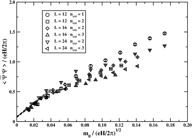
Figure 1: Scaled chiral condensate versus the scaling variable $x$. The continuum line is the linear fit of the data in the scaling region $0<x\lesssim 0.04$.

We see that the continuum scaling law is satisfied for $0<x\lesssim 0.04$. This allows us to extract the chiral condensate in the chiral limit, $x\rightarrow 0$, by the following linear relation:

$$y\;=\;a_{0}\,+\,a_{1}\,x\ .$$ (12)

The best fit of the data to Eq. (12), in the scaling region, gives

$$a_{0}\,=\,0.07668\,\pm\,0.00930\;\;,\qquad a_{1}\,=\,11.20\,\pm\,0.48\ .$$ (13)

As a consequence, we see that in the chiral limit the external magnetic field does induce a non-zero chiral condensate. From Eq. (11) and the result in Eq. (13), restoring cgs units, we find:

$$\langle\overline{\Psi}\Psi\rangle\;=\;\frac{\hbar ceH}{2\pi}\left(0.07668\,\pm\,0.00930\right)\,.$$ (14)

The non-zero value of the chiral condensate can be interpreted as the generation of a dynamical fermion mass $m_{\text{dyn}}$ with gap $\Delta_{0}=m_{\text{dyn}}c^{2}$. To extract $\Delta_{0}$ we use Eq. (10) combined with Eq. (14):

$$\Delta_{0}\;\simeq\;\,-\,\frac{\sqrt{\pi}}{N_{f}\zeta(\frac{1}{2})}\sqrt{\frac{\hslash ceH}{2\pi}}\left(0.07668\,\pm\,0.00930\right)\,.$$ (15)

5 Application to graphene

The graphene is a single sheet of carbon atoms characterised by a honeycomb lattice described by two interpenetrating triangular Bravais lattices. The unit cell is instead a rhombus containing two carbon atoms. The reciprocal lattice comes out to be a hexagonal as well but, between the six corners of the Brillouin zone, only two points are inequivalent (i.e. not connected by a reciprocal lattice vector) and are labelled by $K$ and $K^{\prime}$, called “valleys”.

A simple tight-binding model [12] shows that the dispersion relation $E(\mathbf{k})$ goes to zero at $K$ and $K^{\prime}$. Everywhere else in momentum space $E(\mathbf{k})\neq 0$ and we have two graphene bands, conduction and valence, lying symmetrically above and below the Fermi energy at $E=0$. Therefore, the Fermi level is placed between the two symmetrical bands, with zero excitation energy needed to excite an electron from just below the Fermi energy to just above the six points of the corners of the Brillouin zone.

Moreover, the dispersion relation turns out to be linear near the $K$ and $K^{\prime}$ points: $E(\mathbf{k})=\pm\hslash v_{F}|\mathbf{k}|$, where $v_{F}$ is the Fermi velocity. As discussed in Ref. [13], this yields an effective Hamiltonian made of two copies of Pauli spinors which satisfy the massless two-dimensional Dirac equation with the speed of light replaced by the Fermi velocity.

When graphene is immersed in a transverse magnetic field $H$ the energy levels are quantised into non-equidistant Landau levels:

$$E_{n}=\mbox{sign}(n)\sqrt{2\hslash eH|n|\frac{v_{F}^{2}}{c}},\quad n=0,\pm 1,\ldots\ .$$ (16)

The presence of the “anomalous” Landau level at zero energy leads to half-integer Quantum Hall (QH) effect; the Hall resistance is given by $R_{xy}=h/(e^{2}\nu)$, where the quantised filling factor $\nu$ is:

$$\nu=\pm g_{s}(N+\frac{1}{2})=\pm 2,\pm 6,\pm 10,\dots\ .$$ (17)

The factor $g_{s}=4$ takes into account the spin and valley degeneracy and $\pm$ stands for electron and holes, respectively.

Recently, it has been shown [14] that for very strong magnetic field ($H\gtrsim 20\,T$) new QH states appear corresponding to $\nu=0,\pm 1,\pm 4$. This means that the $n=0$ Landau level is totally resolved into $\nu=0,\pm 1$ plateaus, while the fourfold degeneracy in the $n=\pm 1$ Landau levels is only partially resolved into $\nu=\pm 4$ leaving a twofold degeneracy [14].

The new plateaus at $\nu=0,\pm 4$ can be explained by Zeeman spin splitting; $\nu=\pm 1$ can be explained if there is some kind of generation of a gap $\Delta_{0}$, i.e. a valley symmetry breaking in $n=0$ Landau level [14, 15].

In Ref. [15] the authors determine experimentally the $\Delta E(\nu=1)$ dependence from the magnetic field: they find for it a $\sqrt{H}$ behaviour.

We have fitted the experimental data from Ref. [15] to

$$\Delta E(\nu=1)=2\,\left(\Delta_{0}(H)\,-\,\frac{g}{2}\mu_{B}\,H\right)\ ,$$ (18)

where $\mu_{B}$ is the Bohr magneton, $g=2$ and $\Delta_{0}(H)\sim\sqrt{H}$ (note that the second term takes into account the Zeeman effect); we find:

$$\Delta_{0}(H)\,=\,(13.57\,\pm 0.28)\;{\rm K}\times k_{B}\;\sqrt{H(T)}\ ,$$ (19)

where $k_{B}$ is the Boltzmann factor and $H(T)$ stands for the magnetic field expressed in Tesla.

It is believed that the generation of the gap is driven by the electron-electron interaction (for a review see Ref. [16]); in this picture, the value of the gap is expected to be of the order:

$$\Delta_{0}(H)\approx\frac{e^{2}}{\epsilon}\sqrt{\frac{eH}{\hslash c}}\approx 163K\times k_{B}\sqrt{H(T)}\ ,$$ (20)

i.e. this result is one order of magnitude bigger than the experimental result of Eq. (19).

On the other hand, in Ref. [11] it is supported that the origin of the gap is related to a dynamical generation related to the presence of the magnetic field; this means that we can derive the value of the gap by our numerical results.

The implied hypothesis here is that the Coulomb interaction between the electrons can be neglected because the dominant effect is the magnetic catalysis; this is the reason why we can apply planar QED directly to describe the graphene, although in the literature the Coulomb interaction is always considered as a $3d$ field acting on $2d$ fermions.

To apply our results to graphene, we must simply replace the speed of light $c$ with the Fermi velocity $v_{F}$ in Eq. (15) [11]:

$$\Delta_{0}\;\simeq\;\,-\,\frac{\sqrt{\pi}}{N_{f}\zeta(\frac{1}{2})}\sqrt{\frac{\hslash\frac{v_{F}^{2}}{c}eH}{2\pi}}\left(0.07668\,\pm\,0.00930\right)\ .$$ (21)

It is worth mentioning that the small gap approximation, which we are using here, is correct when it is satisfied the following relation:

$$\frac{\Delta_{0}}{\sqrt{H(T)}}\ll\sqrt{2\hslash v_{F}^{2}e/c}\approx 420K\times k_{B}\ ;$$ (22)

the experimental value found in Eq. (19) is actually small compared with that in Eq. (22), therefore we can consider the small gap approximation valid in this context.

Finally, using the experimental value for the Fermi velocity ($v_{F}\approx 1.0\times 10^{8}$cm/s) in Eq. (21), we get :

$$\Delta_{0}(H)\,=\,(5.52\,\pm 0.67)\;{\rm K}\times k_{B}\;\sqrt{H(T)}\ .$$ (23)

This result can be compared directly with Eq. (19). Since the two values are of the same order of magnitude, our result also confirm our hypothesis that the Coulomb interaction between electrons is actually negligible in presence of an external magnetic field.

6 Conclusion

Our nonperturbative Monte Carlo simulations have shown that the external magnetic field gives rise to a spontaneous breaking of the chiral symmetry. We think that it is possible to apply our results to describe the breaking of the valley symmetry in graphene under strong magnetic field and we determine the numerical value of the gap that compares quite well with the experimental value.

References

- [1] A. Zee, “Quantum field theory in a nutshell,” Princeton, UK: Princeton Univ. Pr. (2010) 576 p.
- [2] S. Hands, C. Strouthos, Phys. Rev. B78 (2008) 165423. [arXiv:0806.4877 [cond-mat.str-el]].
- [3] J. E. Drut, T. A. Lahde, [arXiv:0807.0834 [cond-mat.str-el]].
- [4] P. Cea, L. Cosmai, Phys. Rev. D60 (1999) 094506. [hep-lat/9903005].
- [5] P. Cea, L. Cosmai, JHEP 0508 (2005) 079. [hep-lat/0505007].
- [6] J. Alexandre, K. Farakos, S. J. Hands, G. Koutsoumbas, S. E. Morrison, Phys. Rev. D64 (2001) 034502. [hep-lat/0101011].
- [7] R. Fiore et al., Phys. Rev. D72 (2005) 094508. [hep-lat/0506020].
- [8] P. Cea, L. Cosmai, M. D’Elia, JHEP 0402 (2004) 018. [hep-lat/0401020].
- [9] P. Cea, L. Tedesco, J. Phys. G G26 (2000) 411-429. [hep-th/9909029].
- [10] V. P. Gusynin, V. A. Miransky, I. A. Shovkovy, Phys. Rev. Lett. 73 (1994) 3499-3502. [hep-ph/9405262].
- [11] P. Cea, [arXiv:1101.5703 [cond-mat.mes-hall]].
- [12] P.R. Wallace, Phys. Rev. 71 (1947) 622.
- [13] G.W. Semenoff, Phys. Rev. Lett. 53 (1984) 5449.
- [14] Y. Zhang et al., Phys. Rev. Lett. 96, 136806 (2006).
- [15] Z. Jiang et al., Phys. Rev. Lett. 99, 106802 (2007).
- [16] V. N. Kotov, B. Uchoa, V. M. Pereira, A. H. C. Neto, F. Guinea, [arXiv:1012.3484 [cond-mat.str-el]].