Adiabatic quantum algorithm for search engine ranking

Abstract

We propose an adiabatic quantum algorithm for generating a quantum pure state encoding of the PageRank vector, the most widely used tool in ranking the relative importance of internet pages. We present extensive numerical simulations which provide evidence that this algorithm can prepare the quantum PageRank state in a time which, on average, scales polylogarithmically in the number of webpages. We argue that the main topological feature of the underlying web graph allowing for such a scaling is the out-degree distribution. The top ranked $\log(n)$ entries of the quantum PageRank state can then be estimated with a polynomial quantum speedup. Moreover, the quantum PageRank state can be used in “q-sampling” protocols for testing properties of distributions, which require exponentially fewer measurements than all classical schemes designed for the same task. This can be used to decide whether to run a classical update of the PageRank.

Introduction.—Quantum mechanics provides computational resources that can be used to outperfom classical algorithms Nielsen and Chuang (2004). Problems for which a polynomial or exponential quantum speed-up is achievable have been sought in quantum computation since its inception, and their ranks are swelling slowly Bacon and van Dam (2010). Yet, while ranking the results obtained in response to a user query is one of the most difficult tasks in searching the web Manning et al. (2008), so far no efficient quantum algorithms have been proposed for this task old .

Here we present an adiabatic quantum algorithm Farhi et al. (2000) which prepares a state containing the same ranking information as the PageRank vector. The latter is a central tool in data mining and information retrieval, at the heart of the success of the Google search engine Brin and Page (1998); Manning et al. (2008); Langville and Meyer (2006); Bonato (2008); Berkhin (2005). The best available classical algebraic and Markov Chain Monte Carlo (MCMC) techniques used to evaluate the full PageRank vector require a time which scales as $O(n)$ and $O(n\log n)$, respectively, where $n$ is the number of pages, i.e., the size of the web-graph. We investigate the size of the gap of the adiabatic Hamiltonian numerically using a wide range of web-graph sizes ($n\in\{2^{2},\dots,2^{14}\}$), and present evidence that our quantum algorithm prepares the PageRank state in a time which scales on average as $O[\textrm{polylog}(n)]$. We argue that while extraction of the full PageRank vector cannot in general be done more efficiently than when using the aforementioned classical algorithms, there are particular graph-topologies and specific tasks of relevance in the use of search engines for which the quantum algorithm, combined with other known quantum protocols Aharonov and Ta-Shma (2003); Bravyi et al. (2011); Brassard et al. ; Buhrman et al. (2001), may provide a polynomial, or even exponential speedup. We discuss the underlying graph structure which we believe is responsible for this potential speedup, and provide evidence that it is the power law distribution of the out-degree nodes that plays the key role. A proof of this fact would be very interesting.

Model of the web-graph.—The PageRank algorithm, introduced by Brin & Page Brin and Page (1998), is probably the most prominent ranking measure using the query-independent hyperlink structure of the web. The PageRank vector is the principal eigenvector of the so-called Google matrix, which encodes the structure of the web-graph via its adjacency matrix. The humongous size of the World Wide Web (WWW), with its ever growing number of pages and links, makes the evaluation of the PageRank vector one of the most demanding computational tasks ever Berkhin (2005). In practice PageRank is evaluated over real data providing the structure of the actual WWW. On the other hand the use of models of the web-graph has proved to be useful in testing new ideas concerning structure measures and dynamical properties of the web Bonato (2008). To accurately capture the WWW graph a good candidate model network should be (i) sparse (the number of edges is proportional to the number of nodes), (ii) small-world (the network diameter scales logarithmically in the size of the network), and (iii) scale-free (the in- and out-degree probability distributions obey a power law). To analyze the scaling properties of our algorithm we used two well known models of the web-graph: the preferential attachment model Barabasi and Albert (1999), and the copying model Kleinberg et al. (1999). These models are based on two different network evolution mechanisms, both of which yield sparse random graphs with small-world and scale-free (power-law) features.

We implemented a version Bollobás et al. (2001) of the preferential attachment model that provides a scale-free network with $N(d)\propto d^{-3}$, where $N(d)$ is the number of nodes of degree $d$.

The copying model Kleinberg et al. (1999) improves upon the preferential attachment model by exploiting only local structure to generate a power-law degree distribution, and providing for random graphs with $N(d)\propto d^{(2-p)/(1-p)}$, where $p$ is a probability sup .

Google matrix and PageRank.—PageRank can be seen as the stationary distribution of a random walker on the web-graph, which spends its time on each page in proportion to the relative importance of that page Langville and Meyer (2006).

To model this define the transition matrix $P_{1}$ associated with the adjacency matrix $A$ of the graph

$$P_{1}(i,j)=\left\{\begin{array}[]{ll}1/d(i)&\mbox{if $(i,j)$ is an edge of $A$};\\ 0&\mbox{else},\end{array}\right.$$ (1)

where $d(i)$ is the out-degree of the $i$th node.

Since the out-degree of a node might be $0$, a walker that follows only links can become trapped in a node with no out-links. Equivalently, if $P_{1}$ has a row of all $0$’s then it is not stochastic. To overcome this problem one modifies $P_{1}$ by replacing every zero row with the vector $\vec{e}/n$ whose entries are all $1/n$. Call this new stochastic matrix $P_{2}$. However, there is still the possibility of “importance sinks,” meaning subgraphs with in-links but no out-links, i.e., $P_{2}$ needs to be made irreducible com . To accomplish this one defines the Google matrix $G$ as

$$G:=\alpha P_{2}^{T}+(1-\alpha)E,$$ (2)

where $E\equiv|\vec{v}\rangle\langle\vec{e}|$.

The “personalization vector” $\vec{v}$ is a probability distribution with all positive entries; the typical choice is $\vec{v}=\vec{e}/n$. The parameter $\alpha$ is the probability that the walker follows the link structure of the web-graph at each step, rather than hop randomly between graph nodes according to $\vec{v}$. Google reportedly uses $\alpha=0.85$, which we also use in this work. The matrix $E$ makes $G$ irreducible and aperiodic, and hence the Perron-Frobenius theorem ensures the existence of a unique eigenvector with all positive entries associated to the maximal eigenvalue $1$. This eigenvector is precisely the PageRank $\vec{p}$ Langville and Meyer (2006). Moreover, the modulus of the second eigenvalue of $G$ is upper-bounded by $\alpha$ gap . This is important for the convergence of the power method, the standard computational technique employed to evaluate $\vec{p}$. It uses the fact that for any probability vector $\vec{p}_{0}$

$$\vec{p}=\lim_{k\rightarrow\infty}G^{k}\vec{p}_{0}.$$ (3)

The power method computes $\vec{p}$ with accuracy $\nu$ in a time $O[sn\log({\nu})/\log(\alpha)]$, where $s$ is the sparsity of the graph (maximum number of non-zero entries per row of the adjacency matrix). The rate of convergence is determined by $\alpha$. The other technique used in the evaluation of PageRank is MCMC, where a direct simulation of rapidly mixing random walks is used to estimate the PageRank at each node. The typical running time is $O[n\log(n)]$ Bahmani et al. (2010).

Adiabatic quantum computation.—Even though classical PageRank computation time scales modestly with the problem size $n$, in practice its evaluation for the actual WWW already takes weeks, a time which can only be expected to grow if current computational methods remain the norm, given the rapid pace of expansion of the web. Furthermore, it is often desirable to have multiple personalization vectors, which means that more than one PageRank needs to be evaluated for each WWW graph instance. Considering also the fact that the web-graph is an evolving dynamic entity, it is clear that it is important to speed up the computation of the PageRank in order to provide up-to-date results from the ranking algorithm.

We now show how adiabatic quantum computation (AQC) Farhi et al. (2000, 2001); Roland and Cerf (2002); Young et al. (2008); Dickson and Amin (2011) might be able to help in the optimization of the resources needed to provide an up-to-date PageRank.

Small-scale experiments with the potential to pave the way toward laboratory realization of AQC, involving $8$ superconducting flux qubits, have recently been reported Johnson et al. (2011). In AQC one encodes the solution to a difficult problem in the ground state of a related problem Hamiltonian $H^{(p)}$. The latter is arrived at by slowly modifying an initial Hamiltonian $H^{(i)}$, for which the ground state is—by construction—easy to obtain. The adiabatic evolution is generated by $H(s)=(1-s)H^{(i)}+sH^{(p)}$. If the modification from the initial to the final Hamiltonian is done slowly enough, and the parameter $s(t):0\mapsto 1$ has a smooth time dependence, where the time $t\in[0,T]$, then the quantum adiabatic theorem guarantees that the state of the system will be the ground state for all $t$ with high probability Teufel (2003). More precisely, in order for the final system state $|\psi(T)\rangle=\mathcal{T}e^{-i\int_{0}^{T}H{[}s(t){]}dt}|\psi(0)\rangle$ to have fidelity

$$f:=|\langle\psi(T)|\pi\rangle|\gtrsim 1-\eta^{a}$$ (4)

with respect to the the desired ground state $|\pi\rangle$ of $H^{(p)}$, the total adiabatic evolution time should satisfy

$$T\gtrsim{a}\frac{\Lambda^{b-1}}{\eta\delta^{b}},$$ (5)

where $\Lambda=\max_{s}\|dH/ds\|$ (the norm is the largest eigenvalue) and $\delta=\min_{s}\Delta(s)$, where $\Delta(s)$ is the instantaneous energy gap of $H(s)$ between the ground and first excited state. The values of the integer exponents $a$ and $b$ in Eqs. (4) and (5) depend upon the differentiability and analyticity properties of $H(s)$, and the boundary conditions satisfied by its derivatives; typically $b\in\{1,2,3\}$ Jansen et al. (2007), while $a$ can be tuned between $1$ and arbitrarily large integer values, equal to the number of vanishing derivates of $H(s)$ at the boundaries $s=0$ and $s=1$ ad .

Adiabatic quantum PageRank algorithm.— Since $G$ is not reversible we cannot directly apply the standard technique of mapping it to a discriminant matrix without a priori knowledge of the stationary state Szegedy (2004); Aharonov and Ta-Shma (2003); Krovi et al. (2010). Instead, let us consider the following non-local problem Hamiltonian associated with a generic Google matrix $G$ (note that we use $H$ and $h$ for local and non-local Hamiltonians, respectively):

$$h^{(p)}=h(G)\equiv\left(\mathbb{I}-G\right)^{\dagger}\left(\mathbb{I}-G\right).$$ (6)

Since $h(G)$ is positive semi-definite, and $1$ is the maximal eigenvalue of $G$ associated with $\vec{p}$, it follows that the ground state of $h(G)$ is given by $|\pi\rangle\equiv\vec{p}/\|\vec{p}\|_{2}$. The initial Hamiltonian has a similar form, but it is associated with the Google matrix $G_{c}$ of the complete graph pag

$$h^{(i)}=h(G_{c})\equiv\left(\mathbb{I}-G_{c}\right)^{\dagger}\left(\mathbb{I}-G_{c}\right).$$ (7)

The ground state of $h^{(i)}$ is $|\psi(0)\rangle=\sum_{j=1}^{n}|j\rangle/\sqrt{n}$, a fully delocalized, uniform quantum superposition state. The basis vectors $|j\rangle$ span the $n$-dimensional Hilbert space of $\log n$ qubits. The interpolating adiabatic Hamiltonian is

$$h(s)=(1-s)h^{(i)}+sh^{(p)}.$$ (8)

Equations (6)-(8) completely characterize the adiabatic quantum PageRank algorithm, apart from the interpolation function $s(t)$, which can be optimized using differential geometric or variational methods to simultaneously minimize the adiabatic evolution time $T$ and the adiabatic error $\varepsilon:=\sqrt{1-f^{2}}$ Rezakhani et al. (2009, 2010, 2010). By simulating the dynamics generated by $h(s)$ we can estimate the parameters in Eq. (5) sim .

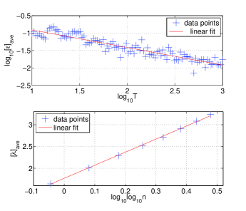
Figure 1: (color online) Top panel: The typical adiabatic error $[\varepsilon]_{\textrm{ave}}$ scales approximately as $T^{-0.48}$. Results are for a system of size $n=16$ (we checked different sizes obtaining similar results), averaged over 100 random web-graph realizations. Bottom panel: $[\lambda]_{\textrm{ave}}$ scales as $\log\log n$, with a prefactor which is approximately 3. Results were averaged over $1000$ random web-graph realizations. See text for more details.

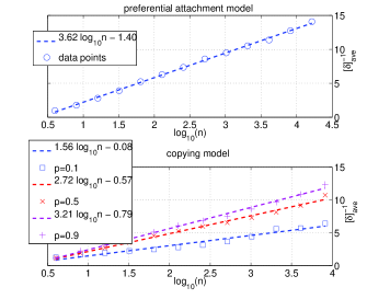
Figure 2: (color online) Scaling of the inverse of the average minimum gap, $1/[\delta]_{\rm ave}$, for the preferential attachment model (top panel), and copying model (bottom panel). We checked numerically that the same logarithmic scaling holds for the averaged inverse gap $[1/\delta]_{\rm ave}$, with the latter slightly larger than $1/[\delta]_{\rm ave}$ for all graph sizes $n$ sup . Note that for the copying model the parameter $p$, relative to the in-degree distribution, affects only the prefactor of the scaling.

Simulation results.—Figures 1 and 2 summarize our numerical simulations on the USC high-performance cluster clu . Figure 1 shows the results for the preferential attachment model, providing information on the adiabatic error $\varepsilon$ and the scaling of $\lambda\equiv\|dh/ds\|=\|{h}^{(p)}-{h}^{(i)}\|$ [corresponding to the numerator in Eq. (5)], with respect to the number of web-graph nodes. In these simulations we made no attempt to minimize the error by optimizing $s(t)$. From the upper panel we can conclude that the adiabatic run-time $T$ scales as the inverse square of the adiabatic error $\varepsilon$. The bottom panel shows the ensemble average of $\lambda$. The fit clearly shows that for the preferential attachment model $\lambda$ exhibits a double logarithmic scaling as a function of $n$. We checked numerically that similar results hold also for the copying model (not shown).

Figure 2 displays the scaling of the minimum gap with respect to system size, also averaged over $1000$ random web-graph realizations. The top panel displays the results for the preferential attachment model. The bottom panel is for the copying model, for which we considered different values of the parameter $p$. In both models the random graphs were generated so that they have both in- and out-degree power-law distributions. More specifically, we mixed (i.e., added the adjacency matrices of) graphs $\mathcal{G}_{A}$, with only in-degree power-law distributions, with graphs $\mathcal{G}_{B}$ with only out-degree power-law distributions. For the simulations reported here, the maximum out-degree for $\mathcal{G}_{B}$ is approximately $3$ times greater than the maximum in-degree for $\mathcal{G}_{A}$. Our simulation results, which cover nearly four orders of magnitude of graph sizes, indicate that, for the class of graphs we have considered, the inverse of the average gap is proportional to $\log(n)$.

Putting together the above observations, namely that for a typical graph instance $\lambda\sim{\rm poly}(\log\log n)$, $\delta\sim 1/{\rm poly}(\log n)$, $T\sim\varepsilon^{-c}$ (with $c\approx 2$, see Figure 1), we can conclude from Eq. (5) that the typical run-time of the adiabatic quantum PageRank algorithm scales as

$$T\sim\varepsilon^{-2}(\log\log n)^{b-1}(\log n)^{b},$$ (9)

where $b$ is some small positive integer that depends on the details of the network topology (see Fig. 2). We checked this result by simulating the adiabatic evolution of the system allowing for a run-time $T=\epsilon^{-2}(\log\log n)^{b-1}(\log n)^{b}$, with both $b=2$ and $b=3$ for small graphs (up to 20 nodes), with a fixed small $\epsilon$. For each evolving random graph we found that the final calculated adiabatic error $\varepsilon$ is always upper bounded by $\epsilon$.

Mapping to a local Hamiltonian.—Since the Google matrix $G$ is not sparse, the physical implementation of the $\log n$-qubits Hamiltonian in Eq. (8) can, in general, require many-body interactions with arbitrarily high locality. This problem is similar to one that arises, e.g., in the quantum adiabatic implementation of Grover’s search algorithm Roland and Cerf (2002). A general technique to overcome the non-locality problem is the use of so-called perturbation gadgets, which requires the introduction of ancillary qubits Jordan and Farhi (2008). However, a more direct alternative is to map the dynamics generated by Eq. (8) from the $n$-dimensional Hilbert space into the $n$-dimensional single particle excitation subspace of an effective $2^{n}$-dimensional Hilbert space with $n$ qubits. This correspondence has been used recently in a different context to study the quantum dynamics of biomolecular systems Giorda et al. (2011), and it has also been considered from an experimental perspective Mostame et al. (2011). The new effective adiabatic Hamiltonian is given by

$$H(s)=\sum_{i=1}^{n}h(s)_{ii}\sigma_{i}^{+}\sigma_{i}^{-}+\sum_{i<j}^{n}h(s)_{ij}\left(\sigma_{i}^{+}\sigma_{j}^{-}+\sigma_{j}^{+}\sigma_{i}^{-}\right),$$ (10)

where $h(s)_{ij}$ is the $(i,j)$th matrix element of $h(s)$ as given in Eq. (8), and $\sigma_{i}^{\pm}$ is the Pauli raising or lowering matrix for the $i$th qubit (or web-graph node) sto . The spectral properties of $H(s)$ in the single particle excitation subspace are the same as those of $h(s)$ sup . This implies that the estimate (9) also holds for $H(s)$, and hence one could envision programming $H(s)$ of Eq. (10) onto physical systems such as excitonic quantum dots or flux qubits, where two-qubit coupling has been shown to be sign- and magnitude-tunable Hime et al. (2006); van der Ploeg et al. (2007); Harris et al. (2010). Provided this programming step can be executed in time at most $O(\log n)$, updating the matrix elements $h(s)_{ij}$ is efficient DWa .

At the conclusion of the adiabatic evolution generated by the Hamiltonian in Eq. (10), the PageRank vector $\vec{p}=\{p_{i}\}$ is encoded into the quantum PageRank state $|\pi\rangle=\sum_{i=1}^{n}\sqrt{\pi_{i}}|i\rangle$ of an $n$-qubit system, where $|i\rangle$ is the vector with $1$ in the $i$th entry, and $0$’s in all the others. The probability of finding the only allowed excitation at site $i$ is $\pi_{i}=p_{i}^{2}/\|\vec{p}\|_{2}^{2}$. One can estimate ${\pi_{i}}$ by repeatedly sampling the expectation value of the operator $\sigma^{z}_{i}$ in the final state. The number of measurements $M$ needed to estimate $\pi_{i}$ is given by the Chernoff-Hoeffding bound Hoeffding (1963), allowing us to approximate $\pi_{i}$ with an additive error $e_{i}$ and with $M={\rm poly}(e_{i}^{-1})$. We now discuss tasks for which the quantum ranking algorithm offers a speedup.

Ranking the top.—The fact that the amplitudes of the quantum PageRank state are $\{\sqrt{\pi_{i}}\}$, rather than $\{\sqrt{p_{i}}\}$, is in fact a virtue: we can show that $\forall i$ the total quantum cost is $O[n^{2\gamma_{i}-1}\textrm{polylog}(n)]$ for estimating the rank $\pi_{i}$ with additive error $e_{i}\sim\pi_{i}$, while the corresponding classical cost is at best $O[n^{\gamma_{i}}\log(n)]$ gai . Thus for this task there is a polynomial quantum speedup whenever $\gamma_{i}<1$; our simulations show that this is indeed the case for the top-ranked $\log(n)$ pages.

Comparing successive PageRanks.—Another context for useful applications is “q-sampling” Aharonov and Ta-Shma (2003). Since the classical PageRank algorithm is so costly when applied to the WWW, one would like to develop criteria for when to run it, e.g., after a relevant perturbation to the graph. The adiabatic quantum algorithm can provide, in time $O[{\textrm{polylog}}(n)]$, the pre- and post-perturbation states $|\pi\rangle$ and $|\tilde{\pi}\rangle$ as input to a quantum circuit implementing the SWAP-test Buhrman et al. (2001). To obtain an estimate of the fidelity $|\langle\pi|\tilde{\pi}\rangle|^{2}$ we need to measure an ancilla $O(1)$ times, the number depending only on the desired precision. Whenever some relevant perturbation of the previous quantum PageRank state is observed, one can decide to run the classical algorithm again to update the classical PageRank. Deciding whether two probability distributions—one of which is known—are close, classically requires approximately $\sqrt{n}$ samples Bravyi et al. (2011); Batu et al. (2001). Related quantum algorithms for testing properties of distributions Valiant (2008) have recently been proposed and analyzed Bravyi et al. (2011).

Discussion.—Why do we observe a “large” gap that scales as $O(1/{\rm poly}(\log n))$? The out-degree distribution seems to be the key feature activating the polylogarithmic behavior sup . In support of this claim we have also analyzed two other classes of random graphs: one with only in-degree power-law distribution, the other with only out-degree power-law distribution. In the former we found that the average inverse gap scales polynomially in the system size (“small” gap), while in latter we found the “large” gap, polylogarithmic scaling. On the other hand when the out-degrees are equal to the in-degrees (as for undirected graphs) the gap scaling is again polynomial. The scaling for intermediate cases is determined by the presence or absence of sufficiently many nodes linking to a relevant portion of the graph: the simulations we have reported here show that graphs with approximately three times more out-going than in-coming links in the most connected nodes exhibit the polylogarithmic scaling. Establishing the exact connection between the in- and out-degree distributions and gap scaling is an interesting open problem for future research.

It would also be interesting to formulate a quantum circuit version of our PageRank algorithm. Perhaps the results obtained in Harrow et al. (2009) concerning the efficient solution of linear systems of equations could be used for this purpose.

Acknowledgments.—The authors are particularly grateful to Aram Harrow for insightful comments. Thanks also to Scott Aaronson, Richard Cleve, Hartmut Neven and Robert Kosut for useful discussions. This work was supported by NSF grants No. PHY-969969 and No. PHY-803304 to PZ and DAL. Additional support was provided to DAL by the NASA Ames Research Center, the Lockheed Martin Corporation URI program, and the Google Research Award program.

Appendix A Supplemental material

A.1 Preferential attachment model and copying model

The idea behind the preferential attachment model algorithm is that new vertices are more likely to attach to existing vertices with high degree. In our simulations we implemented the algorithm proposed in Bollobás et al. (2001), where some ambiguities of the original preferential attachment model Barabasi and Albert (1999) were resolved. This algorithm provides a scale-free network having a power-law degree distribution with a fixed exponent equal to $3$: $N(d)\propto d^{-3}$, where $N(d)$ is the number of nodes of degree $d$. A drawback of the preferential attachment model is that global knowledge of the degree of all nodes is required. Moreover, the exponent of the power-law degree distribution is not controllable. The copying model introduced in Kleinberg et al. (1999) overcomes these drawbacks. It exploits only local structure to generate a power-law degree distribution. To do so one starts from a small fixed initial graph of constant out-degree, and at each time step a pre-existing vertex is chosen uniformly at random. This node is called the copying vertex. For each neighbor of the copying vertex, a link is added from a new added vertex to that neighbor with probability $1-p$, while with probability $p$ a link is added from the new added vertex to a uniformly random chosen one. The parameter $p$ allows to obtain random graphs with power-law degree distributions with exponents given by ${(2-p)}/{(1-p)}$.

A.2 Equivalence of non-local and local single-excitation Hamiltonians

Here we show that the spectrum of the $N$-level Hamiltonian (acting on an $N$-dimensional Hilbert space)

$$h=\sum_{i=1}^{N}h_{ii}|i\rangle\langle i|+\sum_{i<j}h_{ij}(|i\rangle\langle j|+|j\rangle\langle i|),$$ (11)

is the same as the spectrum of the following spin Hamiltonian (acting on the Hilbert space of $N$ qubits), when restricted to the single excitation manifold,

$$H=\sum_{i=1}^{N}h_{ii}\sigma^{+}_{i}\sigma^{-}_{i}+\sum_{i<j}^{N}h_{ij}(\sigma^{+}_{i}\sigma^{-}_{j}+\sigma^{+}_{j}\sigma^{-}_{i})$$ (12)

where $\sigma_{k}^{\pm}$ are Pauli ladder operators acting on the $k$th qubit.

Since the Hilbert space of the $N$-qubit Hamiltonian is restricted to the single excitation manifold it is spanned by $N$ basis vectors which can be put into one-to-one correspondence with the basis vector of the Hilbert space of the $N$-level Hamiltonian

$$|i\rangle\leftrightarrow|\uparrow\rangle_{i}\equiv|\downarrow_{1}\cdots\downarrow_{i-1}\;\uparrow_{i}\;\downarrow_{i+1}\cdots\downarrow_{N}\rangle.$$ (13)

Choosing the following representation for the Pauli matrices acting on qubit $j$,

$$\sigma^{x}_{j}=|\uparrow\rangle\langle\downarrow|_{j}+|\downarrow\rangle\langle\uparrow|_{j}$$

$$\sigma^{y}_{j}=i\left(|\downarrow\rangle\langle\uparrow|_{j}-|\uparrow\rangle\langle\downarrow|_{j}\right)$$

$$\sigma^{z}_{j}=|\uparrow\rangle\langle\uparrow|_{j}-|\downarrow\rangle\langle\downarrow|_{j}$$

$$\sigma^{+}_{j}=\frac{\sigma^{x}_{j}+i\sigma^{y}_{j}}{2}=|\uparrow\rangle\langle\downarrow|_{i}$$

$$\sigma^{-}_{j}=\frac{\sigma^{x}_{j}-i\sigma^{y}_{j}}{2}=|\downarrow\rangle\langle\uparrow|_{i},$$ (14)

one can derive Eq. (12) from Eq. (11) using Eq. (13). The spectrum does not change in this construction since we are simply relabeling the bases of two isomorphic Hilbert spaces.

Another way of seeing this is to note that when the Hamiltonian in Eq. (12) is not restricted to the single excitation manifold and one has to diagonalize it, if the excitation numbers are conserved quantities, then one can first reduce the Hamiltonian into blocks labeled by the number of excitations and subsequently diagonalize each single block. The block labeled by a single excitation is equivalent to Eq. (11) via the mapping in Eq. (13).

A.3 Role of the out-degrees

The WWW graph is characterized by a power-law distribution for both for the in- and out-degrees of the nodes. Here we provide numerical evidence supporting the fundamental role played by the out-degrees in activating the polylogarithmic scaling of the average inverse gap, as a function of system size $n$ (the number of vertices in the graph).

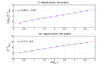
Figure 3: (color online) Top panel: The average inverse minimum gap scaling for random graphs with only in-degree power-law distribution. Bottom panel: The average inverse minimum gap scaling for random graphs with only out-degree power-law distribution. 1000 realizations.

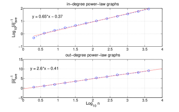
Figure 4: (color online) The inverse of the average minimum gap scaling for undirected preferential attachment random graphs. Top panel: log-log plot. Bottom panel: semi-log plot. Linear fits are poor in both cases. Averaged over 1000 realizations.

In order to distinguish the effect of the in-degrees from that of the out-degrees we consider preferential attachment graphs constructed in such a way that only one power-law is present. Starting with preferential attachment networks with only in-degree power-law distribution, Fig. 3 (top panel) shows the typical behavior of the inverse minimum gap. In this case the scaling is sub-linear, though not logarithmic: $[\delta^{-1}]_{\textrm{ave}}\sim n^{0.65}$. Also shown in Fig. 3 (bottom panel) is the scaling for the reverse graphs, obtained by reversing the direction of each edge. This corresponds to networks in which only the out-degrees are power-law distributed. Remarkably, in this case we find the fit $[\delta^{-1}]_{\textrm{ave}}\sim(\log_{10}n)^{2.7}$. In Fig. 4 we plot the same data considering the inverse of the average minimum gap, instead of the average of the inverse minimum gap. As expected qualitatively the scaling is the same, with small quantitative discrepancies.

Fig. 5 shows what happens when we consider preferential attachment graphs with identical in- and out-degrees. In this case the graph is equivalent to an undirected graph, and we find non-logarithmic, sub-linear scaling. We display both the double-logarithmic and the semi-logarithmic plots in order to make the distinction clear.

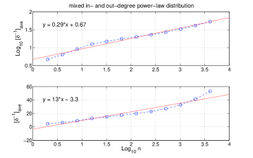
Figure 5: (color online) The average inverse minimum gap scaling for undirected preferential attachment random graphs. Top panel: log-log plot. Bottom panel: semi-log plot. Linear fits are poor in both cases. Averaged over 1000 realizations.

We note that the quantum adiabatic algorithm can still be useful even in the case of networks with only in-degree power-law distribution, for the preparation not of the pagerank state, but of the so-called inverse pagerank Gyongyi et al. (2004) (used for spam detection). The latter is the pagerank of the reverse graph. The results of the simulations in Figs. 3-5 suggest that, typically, when the algorithm is unable to prepare the pagerank in polylogarithmic time, it can still prepare the inverse pagerank in polylogarithmic time.

References

- Nielsen and Chuang (2004) M. A. Nielsen and I. L. Chuang, Quantum Computation and Quantum Information (Cambridge University Press, 2004).
- Bacon and van Dam (2010) D. Bacon and W. van Dam, Commun. ACM, 53, 84 (2010).
- Manning et al. (2008) C. D. Manning, P. Raghavan, and H. Schütze, Introduction to Information Retrieval (Cambridge University Press, New York, NY, 2008).
- (4) Several recent papers have reported a physics approach to the properties of the Google matrix and the PageRank vector, e.g., Perra et al. (2009); Giraud et al. (2009); Georgeot et al. (2010). The focus of this research is mainly on localization phenomena occurring on the web graph, and unlike our work, it does not fully address computational complexity issues.
- Farhi et al. (2000) E. Farhi, J. Goldstone, S. Gutmann, and M. Sipser, eprint quant-ph/0001106 (2000).
- Brin and Page (1998) S. Brin and L. Page, Computer Networks and ISDN Systems, 30, 107 (1998).
- Langville and Meyer (2006) A. N. Langville and C. D. Meyer, Google’s PageRank and Beyond: The Science of Search Engine Rankings (Princeton University Press, 2006).
- Bonato (2008) A. Bonato, A Course on the Web Graph (American Mathematical Society, Boston, MA, USA, 2008).
- Berkhin (2005) P. Berkhin, Internet Mathematics, 2, 73 (2005).
- Aharonov and Ta-Shma (2003) D. Aharonov and A. Ta-Shma, in Proceedings of the 35th annual ACM symposium on theory of computing, STOC ’03 (ACM, New York, NY, USA, 2003) pp. 20–29.
- Bravyi et al. (2011) S. Bravyi, A. Harrow, and A. Hassidim, IEEE Transactions on Information Theory, 57, 3971 (2011).
- (12) G. Brassard, P. Höyer, and M. Mosca, in Quantum Information Science and its Contributions to Mathematics, p.53 (AMS Contemporary Mathematics Series Millennium Volume, Washington, D.C., 2002), arXiv:quant-ph/0005055 .
- Buhrman et al. (2001) H. Buhrman, R. Cleve, J. Watrous, and R. de Wolf, Phys. Rev. Lett., 87, 167902 (2001).
- Barabasi and Albert (1999) A. L. Barabasi and R. Albert, Science, 286, 509 (1999).
- Kleinberg et al. (1999) J. M. Kleinberg, R. Kumar, P. Raghavan, S. Rajagopalan, and A. S. Tomkins, in Computing and Combinatorics (Proceedings of the 5th Annual International Conference, COCOON’99, 1999) p. 1.
- Bollobás et al. (2001) B. Bollobás, O. Riordan, J. Spencer, and G. Tusnády, Random Structures and Algorithms, 18, 279 (2001).
- (17) See Supplemental Material for details on the preferential attachment and copying models, a discussion of the equivalence of the non-local and local single-excitation Hamiltonians, and additional simulation result.
- (18) An irreducible stochastic matrix implies that there exists a directed path from each node to any other node.
- (19) This result only requires both and to be row-stochastic, and to have rank 1 Nussbaum (2003).
- Bahmani et al. (2010) B. Bahmani, A. Chowdhury, and A. Goel, Proc. VLDB Endow., 4, 173 (2010).
- Farhi et al. (2001) E. Farhi, J. Goldstone, S. Gutmann, J. Lapan, A. Lundgren, and D. Preda, Science, 292, 472 (2001).
- Roland and Cerf (2002) J. Roland and N. J. Cerf, Phys. Rev. A, 65, 042308 (2002).
- Young et al. (2008) A. P. Young, S. Knysh, and V. N. Smelyanskiy, Phys. Rev. Lett., 101, 170503 (2008).
- Dickson and Amin (2011) N. G. Dickson and M. H. S. Amin, Phys. Rev. Lett., 106, 050502 (2011).
- Johnson et al. (2011) M. W. Johnson, M. H. S. Amin, S. Gildert, T. Lanting, F. Hamze, N. Dickson, R. Harris, A. J. Berkley, J. Johansson, P. Bunyk, E. M. Chapple, C. Enderud, J. P. Hilton, K. Karimi, E. Ladizinsky, N. Ladizinsky, T. Oh, I. Perminov, C. Rich, M. C. Thom, E. Tolkacheva, C. J. S. Truncik, S. Uchaikin, J. Wang, B. Wilson, and G. Rose, Nature, 473, 194 (2011).
- Teufel (2003) S. Teufel, Adiabatic Perturbation Theory in Quantum Dynamics (Springer-Verlag, Berlin, 2003).
- Jansen et al. (2007) S. Jansen, M.-B. Ruskai, and R. Seiler, J. Math. Phys., 48, 102111 (2007).
- (28) See, e.g., Theorem 1 in Ref. Lidar et al. (2009) for a complete statement, including prefactors omitted in Eqs. (4) and (5).
- Szegedy (2004) M. Szegedy, Annual IEEE Symposium on Foundations of Computer Science, 32 (2004).
- Krovi et al. (2010) H. Krovi, M. Ozols, and J. Roland, Phys. Rev. A, 82, 022333 (2010).
- (31) When the initial Hamiltonian is chosen to be “classical”, i.e., with a ground state equal to , the th node of the web graph, instead of , our simulations show that it takes a time sublinear in , though super-logarithmic, to generate the final ground state.
- Rezakhani et al. (2009) A. T. Rezakhani, W.-J. Kuo, A. Hamma, D. A. Lidar, and P. Zanardi, Phys. Rev. Lett., 103, 080502 (2009).
- Rezakhani et al. (2010) A. T. Rezakhani, D. F. Abasto, D. A. Lidar, and P. Zanardi, Phys. Rev. A, 82, 012321 (2010a).
- Rezakhani et al. (2010) A. T. Rezakhani, A. K. Pimachev, and D. A. Lidar, Phys. Rev. A, 82, 052305 (2010b).
- (35) We used the Krylov subspace method Hochbruck and Lubich (1997) to propagate the Schrödinger equation subject to the Hamiltonian , and exact numerical diagonalization to extract the spectral gap.
- (36) The University of Southern California High Performance Cluster (USC-HPC), or Linux Computing Resource, consists of 785 dual-core/dual-processor nodes and 5 x 16 processors, 64GB, large memory servers, interconnected with Ethernet and 2GB Myrinet backbone, and a 1,990 quad-core or hex-core/dual processor nodes cluster with Ethernet and a 10GB Myrinet backbone.
- Jordan and Farhi (2008) S. P. Jordan and E. Farhi, Phys. Rev. A, 77, 062329 (2008).
- Giorda et al. (2011) P. Giorda, S. Garnerone, P. Zanardi, and S. Lloyd, eprint arXiv:1106.1986 (2011).
- Mostame et al. (2011) S. Mostame, P. Rebentrost, D. I. Tsomokos, and A. Aspuru-Guzik, eprint arXiv:1106.1683 (2011).
- (40) We note that is not stoquastic Bravyi and Terhal (2009), in that for all it has both positive and negative off-diagonal matrix elements in the standard basis.
- Hime et al. (2006) T. Hime, P. A. Reichardt, B. L. T. Plourde, T. L. Robertson, C.-E. Wu, A. V. Ustinov, and J. Clarke, Science, 314, 1427 (2006).
- van der Ploeg et al. (2007) S. H. W. van der Ploeg, A. Izmalkov, A. M. van den Brink, U. Hübner, M. Grajcar, E. Il’ichev, H.-G. Meyer, and A. M. Zagoskin, Phys. Rev. Lett., 98, 057004 (2007).
- Harris et al. (2010) R. Harris, M. W. Johnson, T. Lanting, A. J. Berkley, J. Johansson, P. Bunyk, E. Tolkacheva, E. Ladizinsky, N. Ladizinsky, T. Oh, F. Cioata, I. Perminov, P. Spear, C. Enderud, C. Rich, S. Uchaikin, M. C. Thom, E. M. Chapple, J. Wang, B. Wilson, M. H. S. Amin, N. Dickson, K. Karimi, B. Macready, C. J. S. Truncik, and G. Rose, Phys. Rev. B, 82, 024511 (2010).
- (44) Efficient updating of coupling coefficients is indeed possible. For example, the Rainier chip developed by D-Wave Inc. supports such updating Johnson et al. (2010).
- Hoeffding (1963) W. Hoeffding, J. of the American Statistical Association, 58, 13 (1963).
- (46) We have observed numerically that , where , and that . Let denote the additive error corresponding to , and the additive error corresponding to . It follows from the Chernoff-Hoeffding inequality that the number of samples from the distribution , where (output of the quantum algorithm) or (PageRank) required for a given, fixed additive estimation error, is proportional to the inverse of the additive error: , . Assuming and it follows that , while . The total cost required to prepare the sample in the quantum case is, as we have shown, , while it is at best for classical MCMC for a stochastic matrix with constant gap, as is the case for the Google matrix. Thus, the fact that we have a speedup for estimation of the top- pages is due to the fact that we prepare the distribution rather than . Of course, if the classical algorithm were modified to prepare rather than —presumably by an appropriate modification of —the quantum algorithm could correpondingly be modified to prepare the distribution , etc.
- Batu et al. (2001) T. Batu, L. Fortnow, E. Fischer, R. Kumar, R. Rubinfeld, and P. White, FOCS’01: Proc. 42nd IEEE Symp. Found. Comput. Sci., 442 (2001).
- Valiant (2008) P. Valiant, in Proceedings of the 40th annual ACM symposium on theory of computing, STOC ’08 (ACM, New York, NY, USA, 2008) pp. 383–392.
- Harrow et al. (2009) A. W. Harrow, A. Hassidim, and S. Lloyd, Phys. Rev. Lett., 103, 150502 (2009).
- Perra et al. (2009) N. Perra, V. Zlatić, A. Chessa, C. Conti, D. Donato, and G. Caldarelli, Europhys. Lett., 88, 48002 (2009).
- Giraud et al. (2009) O. Giraud, B. Georgeot, and D. L. Shepelyansky, Phys. Rev. E, 80, 026107 (2009).
- Georgeot et al. (2010) B. Georgeot, O. Giraud, and D. L. Shepelyansky, Phys. Rev. E, 81, 056109 (2010).
- Nussbaum (2003) R. Nussbaum, (2003), arXiv:math/0307056 .
- Lidar et al. (2009) D. A. Lidar, A. T. Rezakhani, and A. Hamma, J. Math. Phys., 50, 102106 (2009).
- Hochbruck and Lubich (1997) M. Hochbruck and C. Lubich, SIAM Journal on Numerical Analysis, 34, 1911 (1997).
- Bravyi and Terhal (2009) S. Bravyi and B. M. Terhal, SIAM J. Comput., 39, 1462 (2009).
- Johnson et al. (2010) M. W. Johnson, P. Bunyk, F. Maibaum, E. Tolkacheva, A. J. Berkley, E. M. Chapple, R. Harris, J. Johansson, T. Lanting, I. Perminov, E. Ladizinsky, T. Oh, and G. Rose, Superconductor Science and Technology, 23, 065004 (2010)
- Bollobás et al. (2001) B. Bollobás, O. Riordan, J. Spencer, and G. Tusnády, Random Structures and Algorithms, 18, 279 (2001).
- Barabasi and Albert (1999) A. L. Barabasi and R. Albert, Science, 286, 509 (1999).
- Kleinberg et al. (1999) J. M. Kleinberg, R. Kumar, P. Raghavan, S. Rajagopalan, and A. S. Tomkins, in Computing and Combinatorics (Proceedings of the 5th Annual International Conference, COCOON’99, 1999) p. 1.
- Gyongyi et al. (2004) Z. Gyongyi, H. Garcia-Molina, and J. Pedersen, (2004), in Proceedings of the 30th International Conference on Very Large Data Bases, Volume 30.