Susy Theories and QCD: Numerical Approaches.

Abstract

We review on-shell and unitarity methods and discuss their application to precision predictions for LHC physics. Being universal and numerically robust, these methods are straight-forward to automate for next-to-leading-order computations within Standard Model and beyond. Several state-of-the-art results including studies of $W$/$Z$+3-jet and $W$+4-jet production have explicitly demonstrated the effectiveness of the unitarity method for describing multi-parton scattering. Here we review central ideas needed to obtain efficient numerical implementations. This includes on-shell loop-level recursions, the unitarity method, color management and further refined tricks.

This article is an invited review for a special issue of Journal of Physics A devoted to “Scattering Amplitudes in Gauge Theories”.

1 Introduction

The physics program at the Large Hadron Collider (LHC) relies heavily on the ever increasing theoretical control over modeling high-energy proton collisions. The detailed theoretical understanding not only increases the reach in new physics and particle searches, but also allows to study the fundamental dynamics and properties of particles. Formulating new observables for addressing specific physics questions is a typical task which relies on quantitative reliable theoretical input. In the long run, high statistics measurements combined with precision prediction from theory will allow systematic probes of fundamental particle theory at ever deeper levels.

The theory of Quantum Chromodynamics (QCD) concisely describes the collisions of protons, however, the dominant dynamics differ depending on observables and the regions of phase-space [1, 2, 3, 4, 5]. Here we have in mind proton collisions with large momentum transfer that are typical for the production of heavy particles. These include the Higgs, top, new particles within theories of supersymmetry as well as more conventional Standard Model processes at large scattering angles. To a good approximation such scattering processes factorize into the long-distance dynamics of quarks and gluons within protons, short distance hard interactions between these partons and, finally, the formation of hadrons and observable jets from the emerging partonic states and remaining proton fragments. Monte Carlo event generators deal with all aspects of the multi-layered simulation of the proton collisions. For some purposes, i.e. sufficiently inclusive observables, it is accurate to use a simpler, purely partonic description of events. To this end one combines final-state partons into observable jets, consistently ignoring corrections from showering and hadronization. Numerical methods are commonly used for the evaluation of differential cross sections, being well suited for comparisons to experimental data.

The hard scattering process is a central stage in the simulation of proton collisions. It is described through scattering amplitudes which are accessible through first principle computations in quantum field theory. The complexity of scattering process allows only a perturbative approach, based on the expansion in the strong coupling $\alpha_{S}(\mu_{R}^{2})$. A first step towards a theoretical understanding of QCD is the evaluation of cross sections at leading order (LO) in the strong coupling $\alpha_{S}(\mu_{R}^{2})$. Many tools [6, 7, 8, 9, 10] are available to generate predictions at leading order. Some of the methods applied incorporate higher-multiplicity leading-order matrix elements into parton-showering programs [11, 12], using matching (or merging) procedures [13, 14].

The truncation of the perturbative expansion introduces an explicit dependence on the unphysical renormalization scale $\mu_{R}$ leading to a theoretical uncertainty. QCD cross sections can have strong sensitivity on higher-order corrections, motivating the challenging quest for perturbative corrections. Next-to-leading (NLO) order predictions significantly reduce renormalization- and factorization-scale dependence – a feature that becomes more significant with increasing jet multiplicity (see e.g. [15]). In addition, NLO corrections take into account further physics effects including initial state radiation, parton merging into jets and a more complete account of partonic production channels. Fixed-order results at NLO can also be matched to parton showers [16] with the prospect of complete event generation at next-to-leading-order in the strong coupling. The value of a first principle understanding of scattering processes in addition to the increased quantitative control motivates the quest for cross sections at NLO and sometimes beyond this [17, 18].

In this contribution we will describe loop-level on-shell [19, 20, 21] and unitarity methods [22, 23]. Our main focus will be on generalized unitarity [24, 25, 26] and its extensions for the numerical computation [27, 28, 21, 29] of hard scattering matrix elements. In addition, we will discuss numerical on-shell loop-level recursions [21]. The central strategy of these approaches is to make maximal use of universal physical principles and mathematical structures in order to describe complex multi-particle processes including quantum corrections. Numerical algorithms based on unitarity and on-shell methods are efficient, numerically stable and can be automated for generic scattering processes. The rapid recent developments in this field have already led to many new studies of complex scattering processes at the LHC [30, 31, 32, 33, 34, 35, 36, 37, 38]. Several further implementations of unitarity methods have been reported [39, 40, 41, 38, 42]. For related analytic approaches see the chapter in this review by Britto [43].

For processes at the LHC with complicated final states, computations can be very challenging. In principle, one can use the traditional Feynman diagram representation of amplitudes for numerical evaluation. However, even at leading order, the number of Feynman diagrams grows more than factorial as the number of final-states increases. Computation times scale accordingly and refined approaches are needed.

At leading order recursive approaches allow to reduce the growth in complexity. Two central strategies are commonly used for numerical computations: Off-shell recursion relations [44, 45, 46], based on Dyson-Schwinger equations, optimise the reuse of recurring groups of Feynman graphs. In contrast, on-shell recursions [47, 48] take advantage of the remarkable simplicity of the physical scattering amplitudes (see e.g. [49]). The simplicity arises in part from symmetry properties of tree amplitudes [50, 51, 52] that are present in QCD-like theories; see the chapter in this review by Brandhuber, Spence and Travaglini [53]. For most practical purposes the efficiency of the two approaches is comparable, depending on the explicit realization of the algorithms.

At next-to-leading-order additional challenges arise, in particular, for the virtual corrections due to the loop-momentum integration. NLO cross sections are built from several ingredients: virtual corrections, computed from the interference of tree-level and one-loop amplitudes; real-emission corrections; and a mechanism for isolating and integrating the infrared singularities in the latter. Automated approaches [54, 55, 56] to deal with these issues are available based on subtraction methods [57, 58, 59]. Recursive methods are effective for computations of real-emission corrections. Such methods, however, are not directly applicable to virtual corrections. Traditional methods evaluate the loop integrals of Feynman diagrams (see e.g. [60, 61, 62]), and have to overcome two central challenges: growth of the number of Feynman diagram expressions and the evaluation of tensorial loop integrals, while maintaining gauge invariance. Means to deal with tensor integral reductions [63, 64] as well as strategies to recycle substructures have been shown to reduce complexity inherent in Feynman diagram approaches [65, 61]. For a more complete discussion of important NLO computations along these lines see ref. [66].

The unitarity method [22], in contrast, constructs loop amplitudes from on-shell tree amplitudes; gauge invariance is built in and maintained throughout computations. In addition, complexity arising from large numbers of Feynman diagrams is avoided by recursive methods for tree evaluations. Similarly, loop-level recursions [19, 20, 67, 21] construct amplitudes efficiently using purely on-shell lower-point input. Effective numerically stable implementations of these on-shell methods have been demonstrated by various groups [21, 68, 35, 40, 39, 41, 38, 42]. Beyond this, unitarity approaches have already been applied to state-of-the-art NLO computations [36, 30, 31, 32, 69, 34, 37].

In more detail, numerical unitarity based approaches use a combination of methods. Scattering amplitudes are naturally split into two parts; a part with logarithmic dependence on kinematic invariants and a rational remainder. Typically, unitarity approaches in strictly four dimensions are used for the computation of the logarithmic parts, although, on-shell recursions [20] may as well be applied in certain cases. At present, there are three main choices for computing the rational remainder within a process-nonspecific numerical program: on-shell recursion [21], $D$-dimensional unitarity [23, 29], and a refined Feynman-diagram approach [70, 38]. We will discuss here numerical unitarity approaches in four and $D$ dimensions following refs. [21, 29] as well as numerical loop-level on-shell methods [21].

Several recent developments allow us to use a purely numerical approach at loop level. A key tool is generalized unitarity [24, 25] which imposes multiple unitarity cuts (more then two propagators) and gives a refined system of consistency relations that is easier to solve. In addition, generalized cuts allow for a hierarchical approach; computing coefficients of four-point integrals, in turn three-point and, finally, two-point etc. integrals from successively cutting four, three and two propagators. (For the related maximal cut technique for multi-loop amplitudes see [71].) Analogous approaches may be applied in $D$ dimensions [23] (see also [72]), where higher point integrals have to be considered. Further simplifications arise from working directly with the loop integrand as opposed to the integrated loop amplitude. The unitarity method then turns into a purely algebraic approach. The starting point for this approach is a generic representation of the loop integrand [27], whose free, process dependent parameters are to be determined by unitarity relations. A particularly useful parametrisation of the loop integrand was given by [27] (see also ref. [28]) and extended in [29] to $D$ dimensions. Importantly, despite the restrictions imposed by on-shell conditions in unitarity cuts, sufficient freedom remains in loop-momentum parametrization in order to uniquely determine all integral coefficients for renormalizable theories and beyond.

Modern on-shell and unitarity methods may be set up to take advantage of refined physical properties and formal structures of scattering amplitudes. We will discuss the uses of structures like spinor helicity [73, 74], analyticity properties, color decomposition [75, 76, 77] and supersymmetry properties [78, 24] in order to make computations efficient. The scattering amplitudes are then decomposed into a fine set of gauge invariant pieces (primitive amplitudes), which are computed individually and eventually assembled into the full matrix element. This approach leads to excellent numerical stability and can be further exploited [32] for caching and efficiency gains through importance sampling (as used in color-expansions). In addition to aiming for efficiency it can be helpful to use methods which are easy to automate within existing frameworks [70, 38] or fulfill further computational constraints [40].

Furthermore, a numerical approach to amplitudes requires attention to numerical instabilities induced by round-off error. A natural way to deal with round-off errors is to setup a rescue system which monitors numerical precision and invokes an alternative computational approach when checks fail. A convenient rescue strategy [79, 21] for unitarity based approaches is the use of higher precision arithmetic. The advantage of a fine split-up of loop amplitudes into gauge invariant subparts is that one can setup a very targeted and thus efficient rescue system.

The present chapter of this review is organized as follows. In section 2 we discuss a representative example for next-to-leading-order multijet computations at hadron colliders pointing out the importance of on-shell and unitarity methods. In section 3 we discuss the key properties of in matrix elements that can be exploited for the computation of loop amplitudes. Finally, numerical unitarity approaches will be discussed in section 4 and loop-level recursions in section 5. We end with conclusions and an outlook.

2 NLO Predictions for Hadron Colliders

As an example, to point out the key features of NLO QCD predictions we will focus on processes of massive vector-boson production in association with jets. In particular, we focus on recent progress due to the use of numerical unitarity approaches.

The production of massive vector bosons in association with jets at hadron colliders has been the subject of theoretical studies for over three decades [80, 81, 82, 83, 84, 85, 86, 87]. These theoretical studies have for example played an important role in the discovery of the top quark [88]. The one-loop matrix elements for $W\,\!+2$-jet and $Z\,\!+2$-jet production were determined [24] via the unitarity method [22] (see also ref. [89]), and incorporated into the parton-level MCFM [90] program. Studies of $W$ production in association with heavy quarks have also been performed [91, 92, 93, 94, 95, 96].

Beyond this, the numerical unitarity approach allowed to include additional final-state objects. Studies of $W\,\!+3$-jet production can be found in [30, 31, 32, 69] and $Z\,\!+3$-jet in [34]. The state-of-the-art in perturbative QCD for hadron colliders are currently parton-level next-to-leading order computations with up to five final-state objects. The first and only such process to be computed so far is $W\,\!+4$-jet production [36]. More generally, several important QCD processes with four final-state objects have been computed to date [97, 35, 98, 37].

Processes of $Z$- and $W$-boson production in association with jets have a particularly rich phenomenology at the electro-weak symmetry breaking scale, being important backgrounds to many searches for new physics and particles, for Higgs physics, and will continue to be important to precision top-quark measurements. Decays of the massive vector-bosons into neutrinos mimic missing energy signals and are of particular importance for supersymmetry searches [99, 100, 101]. The clean leptonic decays of the vector-bosons open a high resolution view of underlying QCD dynamics. Inclusive production cross section provides valuable information about parton distribution functions as well as fundamental parameters of the Standard Model. The signal of vector-boson production in association with jets per se includes physics of jet-production ratios [102] including comparative studies of $W$, $Z$ and photon production. Experimental studies of vector-boson + jet production at the Tevatron were published by the CDF and D0 collaborations [103, 104, 105] as well as at the LHC by the ATLAS collaboration [106].

2.1 Validation & Prediction

Before turning to the theoretical and technical issues it is useful to assess how good the results are by comparing to experimental data. The quantitative impact of NLO corrections can be directly validated against data from Tevatron $p\bar{p}$ collisions.

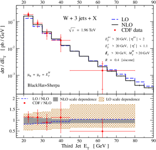
Figure 1: The measured $E_{T}$ distribution of the softest observed jet in inclusive $W\,\!+3$-jet production, compared to the NLO prediction [30, 32]. In the upper panels the NLO distribution is the solid (black) histogram, and CDF data points are the (red) points, whose inner and outer error bars, respectively, denote the statistical and total uncertainties (excluding the luminosity error) on the measurements. The LO predictions are shown as dashed (blue) lines. The lower panel shows the distribution normalized to the full NLO prediction. The scale-dependence bands are shaded (gray) for NLO and cross-hatched (brown) for LO.
Reprinted fig. 1 with permission from [32] p.27. Copyright (2009) by the American Physical Society.

Fig. 1 compares the $E_{T}$ distribution of the third-most energetic jet in CDF data [103] to the NLO and LO predictions for $W\,\!+3$-jet production [30, 32]. (For a similar analysis using a leading color approximation see also [31].) The upper panels of fig. 1 show the distribution itself, while the lower panels show the ratio of the LO value and of the data to the NLO result.The NLO predictions match the data very well, and uniformly with well matching slope. The central values of the LO predictions, in contrast, have different shapes from the data. The change of shape between LO and NLO is attributed to an imprecise scale in the coupling constant, that governs the production of the softest observed jet, in the leading order computation which gets corrected once loop effects are included as discussed in refs. [107, 31].

Scale-dependence bands indicate rough estimates of the theoretical error. Those are obtained by varying the renormalization- and factorization scales by factors of two around a central scale. For such scale variations, the dependence is of the order of $\pm 40\%$ for $W\,\!+3$-jet processes at LO. At NLO, the scale dependence shrinks to $\pm 10\%$, and we obtain a quantitatively reliable answer. A more detailed discussion can be found in refs. [30, 32].

As another example, we consider predictions for the LHC. For the inclusive production of $W+n$ jets, a basic quantity to examine is the $p_{T}$ distribution for the softest observed jet.

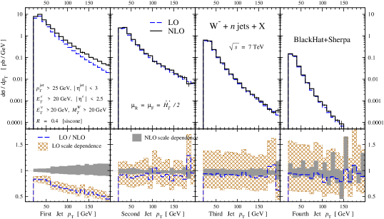
Figure 2: A comparison of the $p_{T}$ distributions of the softest observable jets in $W^{-}$+n-jet ($n=1,2,3,4$) production, respectively. The setup describes the LHC proton-proton collisions at $\sqrt{s}=7$ TeV as published in [36]. In the upper panels the NLO distribution is the solid (black) histogram and the LO predictions are shown as dashed (blue) lines. The lower panels show the LO distribution and LO and NLO scale-dependence bands normalized to the central NLO prediction.

Fig. 2 shows the $p_{T}$ distributions of the softest observed jet in $W^{−}+n$-jet ($n=1,2,3,4$) production at LO and NLO, respectively. For details on our analysis setup we refer to [36]. The predictions are normalized to the central NLO prediction in the lower panels. Comparing the $p_{T}$ distributions successively starting from $W^{−}$+1-jet production, we observe the reduction in differential cross section of about a factor of $\alpha_{S}$ from one panel to the next; each observed jet leads to an additional power in the strong coupling. At the same time the lower panels in fig. 2 show an approximately linear increase in the LO scale variation bands, up to about $\pm 50\%$ for $W\,\!+4$ jets. The scale variation of the NLO result, displayed in the lower panels of fig. 2, is strongly reduced to about $\pm 10\%$ for the present setup.

In summary, in the above examples the advantages of NLO computations over the leading order appear through several quantitative improvements. Firstly, NLO predictions show a greatly reduced dependence on unphysical renormalization and factorization-scales as compared to leading order. The second improvement we pointed out concerns the shapes of distributions. Due to inclusion of radiation from an additional parton as well as a more truthful description of the scale dependence shapes of distributions are modeled better at NLO.

The above results validate our understanding of the $W+n$-jet processes for typical Standard-Model cuts. It will be interesting, and necessary, to explore the size of corrections for observables and cuts used in new-physics searches. A related process that contributes an irreducible background to certain missing energy signals of new physics is $Z\,\!+4$-jet production. We expect that the current setup [36] will allow us to compute NLO corrections to $Z\,\!+4$-jet production, as well as to other complex processes, thereby providing an unprecedented level of theoretical precision for such backgrounds at the LHC.

Parton-level NLO simulations of this kind are first principle predictions whose outcome directly reflect properties of the underlying theory. Although NLO computations are more challenging, in general they yield results with better reliability and agreement with measurements.

2.2 Setup of Complete Computation

The computation of differential distributions is the end product of combining many important ingredients pulled together in a Monte Carlo program; these include parton distribution functions and couplings, phase-space integration, matrix elements, analysis framework etc. Various tools are available to deal with complete NLO computations. One such tool is MCFM [108], which contains an extensive library of analytic matrix elements for NLO computations. Another approach (see [35] and references) uses tools including Helac [7] and CutTools [79] for a numerical approach [27]. Here we will describe another setup [30, 32, 36] based on on-shell and unitarity methods that was used for the computation of $W+n$-jet production in section 2.1.

In addition to LO components of Monte-Carlo programs, at NLO the computations rely on further similarly important ingredients. For the $W+n$-jet production [30, 32, 36] the real-emission and dipole-subtraction terms [58], are provided by the SHERPA package [12]. SHERPA was used to perform phase-space integration. BlackHat was used to compute the real-emission tree amplitudes for $W\,\!+4$jets using on-shell recursion relations [47], along with efficient analytic forms extracted from ${\cal N}=4$ super-Yang-Mills theory [109].

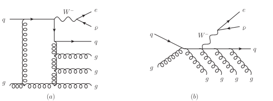
Figure 3: Representative diagrams of matrix elements for $W\,\!+4$-jet production: (a) the eight-point loop amplitudes $qg\rightarrow e\bar{\nu}q^{\prime}ggg$, and (b) the nine-point tree-level amplitudes $qg\rightarrow e\bar{\nu}q^{\prime}gggg$ needed for the real contribution. The $e\bar{\nu}$ pair couples to the quarks via a W boson.

In terms of scattering amplitudes we need the input of up to eight-point one-loop QCD amplitudes as well as up to nine-point tree-level QCD amplitudes; example Feynman diagrams are shown in fig. 3. The squared matrix elements are summed over all initial and final-state partons, parton helicities and color-orderings. For the present computation the $W$-boson is decayed into an observable electron and a neutrino. Amplitudes of this kind can be obtained from QCD amplitudes; with the lepton pair replaced by a quark pair and the $W$-boson exchange related to a gluon exchange. Appropriate dressing with coupling constant and propagator terms are needed. A recent analysis of high multiplicity tree amplitudes of this kind can be found in [109].

3 Structure of One-loop Matrix Elements

The evaluation time of matrix elements is often dominating cross section computations, thus, emphasising the importance of efficient numerical algorithms. Beyond this, matrix elements are objects of fundamental theoretical interest; new physics effects observable at high energy colliders may originate in properties of matrix elements (see e.g. [110]).

Matrix elements are functions of a large number of variables, which characterize particles, polarization states, color quantum numbers, and kinematics. To next-to-leading-order in the strong coupling the parton level cross sections for $(N-2)$ resolved final-state objects, $pp\rightarrow(N-2)$, depend on squared born matrix elements,

$$\sum_{a_{i},h_{i}}{|{\cal A}_{n}^{{\rm tree}}(\{k_{i},h_{i},a_{i}\}|^{2}},\qquad\qquad n=N,N+1\,,$$ (1)

as well as the interference terms,

$$\sum_{a_{i},h_{i}}{{\cal A}_{n}^{{\rm tree}\,*}(\{k_{i},h_{i},a_{i}\}){\cal A}_{n}^{\rm 1\hbox{-}loop}(\{k_{i},h_{i},a_{i}\})}\,+\,c.c.\,,\,\qquad n=N\,,$$ (2)

where $k_{i}$, $h_{i}$, and $a_{i}$ are respectively the momentum, helicity ($\pm$), and color index of the $i$-th external gluon or quark. The shorthand $c.c.$ refers to the complex conjugate part that has to be included. The efficient management of parton and helicity sums is important. For simplicity, we will consider scattering amplitudes involving quarks and gluons only. Much of the methods can be carried over to more general particle spectra.

As inspired by analytic approaches (see e.g.[111]) we disentangle degrees of freedom in order to arrive at a fine set of gauge invariant objects. To this end several structures are used: Color decomposition into color ordered sub amplitudes disentangles color information and kinematics. Use of spinor helicity notation aligns notation of kinematics and polarization vectors. Spinor variables, in addition, lead to a natural way to work in complex momentum space. This in turn allows to exploit analyticity properties of the basic color ordered scattering amplitudes. Use of a standard basis of integral functions will allow a further fine split-up of the loop amplitude into integral functions and their integral coefficients.

Several features motivate us to disentangle matrix elements into a fine set of primitive amplitudes. First of all, do these have cleaner physical and analytic properties than the full matrix elements, as will be discussed in detail below. This can be exploited for the construction of computational algorithms, as will be discussed in detail below. For numerical approaches, a detailed understanding of physical properties (e.g. IR/UV pole structure of primitive amplitudes, or, tensor rank of integrals) allows one to monitor precision and stability of the computation. Furthermore, caching systems built on primitive objects (here, amplitudes) lead to important efficiently gains through reduction of redundant computations. Finally, during numerical phase-space integration, one can introduce importance sampling, computing computationally expensive but numerically small parts on a subset of phase space points.

3.1 Color Decomposition

At tree-level, amplitudes for $SU(N_{c})$ gauge theory with $n$ external gluons can be decomposed into color-ordered partial amplitudes, multiplied by an associated color trace (see e.g. [74]). Summing over all non-cyclic permutations gives the full amplitude,

$${\cal A}_{n}^{\rm tree}(\{k_{i},h_{i},a_{i}\})=\sum_{\sigma\in S_{n}/Z_{n}}\mathop{\rm Tr}\nolimits(T^{a_{\sigma(1)}}\cdots T^{a_{\sigma(n)}})\ A_{n}^{\rm tree}(k_{\sigma(1)}^{h_{\sigma(1)}},\ldots,k_{\sigma(n)}^{h_{\sigma(n)}})\ ,$$ (3)

the coupling is set to one, and $S_{n}/Z_{n}$ is the set of non-cyclic permutations of $\{1,\ldots,n\}$. The $T^{a}$ are the set of hermitian generators of the $SU(N_{c})$ color group. The coefficients of the color structures $\mathop{\rm Tr}\nolimits(T^{a_{1}}\cdots T^{a_{n}})$ define the tree-level color-ordered partial amplitudes, $A_{n}^{\rm tree}(1,2,3,\cdots n)$.

One of the important features of this set of amplitudes is that it forms a closed set under collinear, soft and multi-particle factorization. They have manifest transformation properties under parity transformation and reversal of the ordering of external legs. Similarly, amplitudes with fermions can be decomposed into color-ordered sub-amplitudes [112].

For one-loop amplitudes, one may perform a similar color decomposition to the one at tree-level in eq. (3). In this case, there are up to two traces over color matrices [76],

$${\cal A}_{n}^{\rm 1\hbox{-}loop}\left(\{k_{i},h_{i},a_{i}\}\right)=\sum_{c=1}^{\lfloor{n/2}\rfloor+1}\sum_{\sigma\in S_{n}/S_{n;c}}{\rm Gr}_{n;c}\left(\sigma\right)\,A_{n;c}(\sigma),$$ (4)

where ${\lfloor{x}\rfloor}$ is the largest integer less than or equal to $x$. The leading color-structure factor ${\rm Gr}_{n;1}(1)=N_{c}\ \mathop{\rm Tr}\nolimits\left(T^{a_{1}}\cdots T^{a_{n}}\right)$ is just $N_{c}$ times the tree color factor, and the sub-leading color structures are given by the double trace expressions, ${\rm Gr}_{n;c}(1)=\mathop{\rm Tr}\nolimits\left(T^{a_{1}}\cdots T^{a_{c-1}}\right)\,\mathop{\rm Tr}\nolimits\left(T^{a_{c}}\cdots T^{a_{n}}\right)$. $S_{n}$ is the set of all permutations of $n$ objects, and $S_{n;c}$ is the subset leaving ${\rm Gr}_{n;c}$ invariant.

The leading partial amplitudes $A_{n;1}$ take the form (see e.g. [113]),

$$A_{n;1}^{\rm 1\hbox{-}loop}(1,2,3,\cdots,n)=A_{n}^{\rm g}(1,2,3,\cdots,n)+\frac{n_{f}}{N_{c}}A_{n}^{\rm f}(1,2,3,\cdots,n)\,,$$ (5)

with $A_{n}^{\rm g}$ and $A_{n}^{\rm f}$ being color-ordered sub-amplitudes, or primitive amplitudes. While $A_{n}^{\rm g}$ is fixed to have only gluons propagating in the loop, $A_{n}^{\rm f}$ is restricted to have a Weyl fermion propagating in the loop. The external gluons are color-ordered; the diagrams contributing to the loop amplitudes can be generated from color-ordered Feynman rules, see e.g. ref. [113].

The coefficients of the sub-leading color structures; the sub-leading partial amplitudes, can be expressed in terms of sums [77, 78, 76] of the primitive amplitudes, $A_{n}^{\rm g}$ where different ordering of the external states appear. Beyond the fact that such a decomposition exists, we will not need details of its form here.

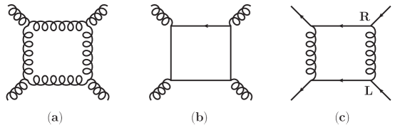
Figure 4: Representative Feynman diagrams for primitive amplitudes with distinct states propagating in the loop: (a) shows a gluon loop of the primitive amplitude $A_{4}^{\rm g}$, (b) a fermion loop of $A_{4}^{\rm f}$ and (c) a mixed fermion/gluon loop of $A_{4}^{\rm LR}$. For the mixed amplitudes (c) we keep track of the routing of the fermion line around the loop; ’$L\,R$’ indicates that the first fermion lines turns left and the second right when entering the loop.

The primitive amplitudes,

$$A_{n}^{\rm g}(1,2,3,\cdots,n)\,\quad\mbox{and}\quad\,A_{n}^{\rm f}(1,2,3,\cdots,n)\,,$$ (6)

form a generating set of amplitudes, such that given these amplitudes, the full one-loop matrix elements can be computed. For fundamental fermions a similar split-up of partial amplitudes is typically more complicated [78, 24]. In addition to the ordering of the external leg the routing around the loop (left- or right-turner) of each of the fermion lines has to be specified. See figure 4 for examples of primitive amplitudes including also external fermion lines.

Primitive amplitudes, have a more transparent analytic structure than full matrix elements, because their external colored legs follow a fixed cyclic ordering. In particular, properties of factorization and branch cut singularities simplify as can be summarized by the following:

1. Only factorization poles and branch cut singularities in adjacent legs appear.

2. Primitive amplitudes and color-ordered tree amplitudes form a closed set under factorization and unitarity cuts.

With the notation specification of ’adjacent legs’ we refer to the fact that factorization poles and unitarity cuts appear only in a specified subset of kinematic invariants $s_{i_{1}\cdots i_{k}}$, with an ordering of momenta identical to the one of external gluons. Closure under factorization means that color ordered amplitudes factorize onto color ordered amplitudes. In particular, for unitarity approaches as well as on-shell recursions, primitive loop amplitudes can be constructed from color-ordered tree amplitudes alone.

For a more complete description of color decomposition we refer the reader to previous reviews [78, 24, 74].

3.2 Structure of Loop Amplitude

Any one-loop amplitude can be written as a sum of terms containing branch cuts in kinematic invariants, $C_{n}$, and a rational remainder $R_{n}$,

$$A_{n}=C_{n}+R_{n}\,.$$ (7)

The cut-containing part $C_{n}$ can in turn be written as a sum over a basis of scalar master integrals [114, 115],

$$C_{n}=\sum_{i_{1}<i_{2}<i_{3}<i_{4}}d^{0}_{i_{1}i_{2}i_{3}i_{4}}\,{\cal I}_{4}^{i_{1}i_{2}i_{3}i_{4}}+\sum_{i_{1}<i_{2}<i_{3}}c^{0}_{i_{1}i_{2}i_{3}}\,{\cal I}_{3}^{i_{1}i_{2}i_{3}}+\sum_{i_{1}<i_{2}}b^{0}_{i_{1}i_{2}}\,{\cal I}_{2}^{i_{1}i_{2}}\,.$$ (8)

The scalar integrals ${\cal I}_{2,3,4}$ – bubbles, triangles, and boxes – are known functions [116]. We omitted tadpole functions, which in dimensional regularization vanish for massless particles circulating in the loop. The explicit dimension dependence is contained in the integral functions with their coefficient functions strictly four dimensional. Feynman diagrams of the integral functions are shown in fig. 5.

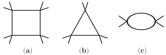
Figure 5: Feynman diagram representation of basis of scalar integrals appearing in the eq. (8): (a) box diagram associated to the 4-point integral, (b) triangle diagram associated to the 3-point integral, and (c) bubble diagram associated to the 2-point integral. Each corner may have one or more external lines attached to it.

The computation of a one-loop amplitude amounts to determining the rational coefficient functions $d^{0}_{i},c^{0}_{j}$ and $b^{0}_{k}$ in addition to the remainder $R_{n}$. Following the spinor-helicity method [73, 81], we can then re-express all external momenta in terms of spinors. The coefficients of these integrals, $d^{0}_{i},c^{0}_{j}$, and $b^{0}_{k}$, as well as the remainder $R_{n}$, are then all rational functions of appropriate spinor and momentum variables.

For the analysis of one-loop amplitudes it is often useful to have two distinct forms of the integrals in mind. One can think of the integral functions as logarithms and polylogarithms of kinematic invariants. As examples we give explicitly a bubble integral function,

$${\cal I}_{2}(s_{12},\hat{\mu}^{2}) = {i\,c_{\Gamma}}\biggl{\{}\frac{1}{\epsilon}+\biggl{(}2+\ln\biggl{(}{\hat{\mu}^{2}\over-s_{12}}\biggr{)}\biggr{\}}+{\cal O}(\epsilon)\,,$$ (9)

exposing discontinuities in kinematic invariants through branch cut singularities of the underlying logarithmic functions. For the kinematic invariants $s_{ij}$ the standard definitions, $s_{ij}=(k_{i}+k_{j})^{2}$, are used. The constant $c_{\Gamma}$ is defined by, $c_{\Gamma}={\Gamma(1+\epsilon)\Gamma^{2}(1-\epsilon)/((4\pi)^{2-\epsilon}\Gamma(1-2\epsilon))}\,.$ The scale $\hat{\mu}$ corresponds to the renormalization and factorization scales which, for convenience, are set to be equal here; $\hat{\mu}=\mu_{R}=\mu_{F}$. The integrals are also viewed as Feynman amplitudes of a scalar field theory,

$${\cal I}_{2}(s_{12},\hat{\mu}^{2}) = \hat{\mu}^{2\epsilon}\int{d^{4-2\epsilon}\ell\over(2\pi)^{4-2\epsilon}}{1\over\ell^{2}(\ell-K_{12})^{2}}\,,$$ (10)

where sums of two momenta are denoted by the shorthand, $K_{ij}=k_{i}+k_{j}$.

3.3 The Loop Integrand

For explicit computations it is useful to consider loop amplitudes before integration, that is to find a universal parametrization  [27, 29] of the loop integrand. In addition to the scalar Feynman diagrams fig. 5, implied from eq. (8), tensorial numerator terms have to included. These tensorial terms describe as well the angular distribution of the virtual particles, which averages out upon integration. The explicit relation between numerator tensors and angular variables will be topic of section 4.3.

A generic form of the loop integrand is given by [27, 29] (see also [28]),

$$A^{{\rm 1\hbox{-}loop},d}_{n}(\ell) = \sum_{i_{1}<\ldots<i_{5}}\frac{\bar{e}_{i_{1}i_{2}i_{3}i_{4}i_{5}}(\ell)}{D_{i_{1}}D_{i_{2}}D_{i_{3}}D_{i_{4}}D_{i_{5}}}+\sum_{i_{1}<i_{2}<i_{3}<i_{4}}\frac{\bar{d}_{i_{1}i_{2}i_{3}i_{4}}(\ell)}{D_{i_{1}}D_{i_{2}}D_{i_{3}}D_{i_{4}}}$$ (11)

$$+\sum_{i_{1}<i_{2}<i_{3}}\frac{\bar{c}_{i_{1}i_{2}i_{3}}(\ell)}{D_{i_{1}}D_{i_{2}}D_{i_{3}}}+\sum_{i_{1}<i_{2}}\frac{\bar{b}_{i_{1}i_{2}}(\ell)}{D_{i_{1}}D_{i_{2}}}\,,$$

where $d$ stands for a given discrete dimension and we restricted external momenta and polarizations to be four-dimensional. If we allow $d$-dimensional polarization vectors and external momenta, higher polygons have to be added in a natural way. The pentagon terms $\bar{e}(\ell)$ should be dropped when working in strictly four dimensions, $d=4$. In the above expression, propagators are denoted by $i/D_{j}=i/(\ell-K_{j})^{2}$; for simplicity, of notation we restrict the discussion on massless internal states. Furthermore, we omitted the single propagator terms $\bar{a}(\ell)$ which drop out of the final results in the absence of massive states. When used with the explicit argument $\ell$ for the loop momentum, $A^{{\rm 1\hbox{-}loop},d}_{n}(\ell)$ denotes the integrand as opposed to the loop amplitude $A^{{\rm 1\hbox{-}loop},d}_{n}$.

The numerators $\bar{e}(\ell),\bar{d}(\ell)$, $\bar{c}(\ell)$, $\bar{b}(\ell)$ and $\bar{a}(\ell)$ are sums of tensors contracted with the loop momentum $\ell^{\mu}$. The tensor-rank is bounded by power-counting. We will refer to these tensors contracted with loop-momentum $\ell$ somewhat imprecisely as numerator tensors. These numerator tensors can be expanded in terms of a basis of tensors in momentum space multiplied by scalar loop-momentum independent coefficients. The scalar coefficients then characterize the loop amplitude. See below in section 3.3.3 for an explicit representation in terms of a basis of tensors and scalar coefficients.

Integrand parametrizations (11) are common in unitarity approaches; for a discussion in the context of multi-loop computations see e.g. refs. [71]. A particularly useful parametrization of the one-loop integrand has been given in [27, 28, 29], as will be discussed further in the following section.

3.3.1 Loop Integration.

With an appropriate representation of the loop integrand the loop integrations can be performed trivially. This is achieved by writing the integrand numerators as a direct sum [27] of terms that integrate to zero and non-vanishing scalar terms. The form of the integrand in eq. (11) then directly relates to the from eq. (8). When we evaluate the known analytic expressions for the basis of integrals, we thus obtain an exact numerical algorithm to go from an off-shell integrand to the integrated loop amplitude. An approach of this kind was used in refs. [27, 21, 28, 29]. We will motivate a canonical form for the loop integrand in this section leaving a more complete discussions to the next. Such a choice can be viewed as an implicit integral reduction procedure.

To have an example in mind, consider the box numerators in the form,

$$\bar{d}_{i_{1}i_{2}i_{3}i_{4}}(\ell) = d^{0}_{i_{1}i_{2}i_{3}i_{4}}+d^{1}_{i_{1}i_{2}i_{3}i_{4}}(n^{1}\cdot\ell)\,.$$ (12)

Here the vector $n^{1}_{\mu}$ is understood to be orthogonal to the external momenta of the box function. (For an explicit definition and properties of $n^{1}_{\mu}$ see later in eq. (17).) The coefficients $d^{0}_{i_{1}i_{2}i_{3}i_{4}}$ and $d^{1}_{i_{1}i_{2}i_{3}i_{4}}$ are the free parameters of the ansatz that have to be determined. The coefficients we eventually need to compute are the coefficients of the scalar term $d^{0}_{i_{1}i_{2}i_{3}i_{4}}$ which correspond to the scalar basis integral coefficients in eq. (8). The tensor coefficient $d^{1}_{i_{1}i_{2}i_{3}i_{4}}$, although necessary at intermediate steps of the computation drops out after integration,

$$\int\frac{d^{4}\ell}{(2\pi)^{4-2\epsilon}}\frac{(n^{1}\cdot\ell)}{D_{i_{1}}D_{i_{2}}D_{i_{3}}D_{i_{4}}}=0\,.$$ (13)

That is, after integration the numerator loop momentum gets replaces by a linear combination of the external momenta $K_{i}$ which are orthogonal to $n^{1}$; giving a vanishing tensor integral.

It is instructive to consider another form of the tensor numerator, including a term with an inverse propagator,

$$\bar{d}_{i_{1}i_{2}i_{3}i_{4}}(\ell) = d^{0}_{i_{1}i_{2}i_{3}i_{4}}+d^{1}_{i_{1}i_{2}i_{3}i_{4}}(n^{1}\cdot\ell)+d^{2}_{i_{1}i_{2}i_{3}i_{4}}D_{i_{1}}\!(\ell)\,.$$ (14)

Clearly the inverse propagator may be cancelled against one of the box propagators turning $d^{2}_{i_{1}i_{2}i_{3}i_{4}}$ into the coefficient of a scalar triangle function. If we were to treat this term at the box level, we obtain tensorial contributions that have to be transcribed into scalar integral functions with some care. Assuming for the moment some prior knowledge about generalized unitarity cuts we can make some further observations. That is, this term actually vanishes on the quadruple cut, leaving the coefficient $d^{2}_{i_{1}i_{2}i_{3}i_{4}}$ unspecified at first. It may then be fixed using the triple-cut equations, although only the sum of the scalar triangle and $d^{2}_{i_{1}i_{2}i_{3}i_{4}}$ may be fixed. The numerical unitarity relations eq. (51) are then not triangular. Then box, triangle and bubble coefficients cannot be solved for consecutively. This is of course obvious in the present example, given that we rewrote a scalar triangle coefficient in box-form. This observation emphasises the need for a good basis of numerator tensors.

A less trivial deformation of the numerator tensors would be to mix in a propagator term with the linear tensor,

$$\bar{d}_{i_{1}i_{2}i_{3}i_{4}}(\ell) = d^{0}_{i_{1}i_{2}i_{3}i_{4}}+d^{1}_{i_{1}i_{2}i_{3}i_{4}}\biggl{(}D_{i_{1}}\!(\ell)+(n^{1}\cdot\ell)\biggr{)}\,.$$ (15)

Here again a scalar triangle contribution is pulled back into the box integral. This time the triangular nature of the cut-equations (see below in eq. (51) for the explicit form of the cut-equations) stays intact and no redundancy is introduced into the numerator tensors. However, one has to pay attention not to drop the coefficient when integrating the tensor box integrals. We can read off the box coefficient directly, $d^{0}_{i_{1}i_{2}i_{3}i_{4}}$, and in addition, we have to include $d^{1}_{i_{1}i_{2}i_{3}i_{4}}$ to the related triangle coefficient.

Terms may be moved around between integral functions in this way, effectively introducing a change of basis of integral functions. As a non-trivial application, a cut completion, that is a subtraction of gram-determinant poles, may be achievable in this way. The form of the numerator tensors has important implication; it allows to keep the unitarity relations triangular, and, keeps the integration of the loop integrand simple.

3.3.2 Numerator Tensors.

In the numerical unitarity approach one is naturally lead to obtain equations for the integrand expression eq. (11). It is then convenient to use an explicit form of the numerators in terms of a basis of tensors. Computing a loop amplitude then amounts to determining the free tensor coefficients.

There are several natural requirements [27] for a good basis of numerator tensors. The first requirement is, that numerator tensors should of course be general enough to parametrize the loop-integrand we are interested in. Typically one uses all tensors up to a given rank, as determined by power-counting. Furthermore, optimally one would like to use a minimal set of tensors. A last requirement is then, that it should be easy to relate the integrand basis back to the integral representation in  eq. (8). It turns out that an optimal tensor basis can be found, which satisfies all the above requirements [27, 28, 29].

For numerator tensors in strictly $d$ dimensions the tensor basis looks particularly simple. (We will discuss the $D$-dimensional generalizations below in section 4.8.) In fact, the result will be a basis of tensors, called spurious numerators in the literature [27], which integrate to zero,

$$0 = \hat{\mu}^{2\varepsilon}\int\frac{d^{4-2\varepsilon}\ell}{(2\pi)^{4-2\varepsilon}}\frac{n_{\mu_{1}\cdots\mu_{k}}\ell^{\mu_{1}}\cdots\ell^{\mu_{k}}}{\ell^{2}(\ell-K_{1})^{2}\cdots(\ell-K_{1}\cdots-K_{n-1})^{2}}\,,\quad k>0\,,$$ (16)

where $n_{\mu_{1}\cdots\mu_{k}}$ stands for a representative basis tensor. Upon integration, the loop-momentum dependent numerators in eq. (11) may thus be dropped and the remaining scalar (rank-zero) terms are directly identified with the integral coefficients in (8).

In order to obtain this basis of tensors it is convenient to introduce the Neerven-Vermaseren basis [115] for vectors in momentum space; a distinct basis for each of the integral functions. Each integral defines a distinguished set of momenta; the momenta $K_{i}^{\mu}$ in eq. (16). Momentum space is decomposed into the direct sum of two subspaces; the physical space parametrized by $K_{i}^{\mu}$ and its complement, spanned by the vectors $n^{i\mu}$ [28],

$$K_{i}\quad\mbox{for}\quad i\in\{1,\cdots,n-1\}\,,\quad\quad n^{i}\quad\mbox{for}\quad i\in\{1,\cdots,d-(n-1)\}\,,$$

$$n^{i}\cdot n^{j}=\delta^{ij}\,,\quad n^{i}\cdot K_{j}=0\,,$$

$$v^{i}\quad\mbox{for}\quad i\in\{1,\cdots,n-1\}\,,\qquad K_{i}\cdot v^{j}=\delta_{i}^{j}\,,\quad n^{i}\cdot v^{j}=0\,,$$ (17)

where we assumed $n\leq d$. For the complementary case $n>d$ momentum space is parametrized solely in terms of a linearly independent set of vectors $K_{i}^{\mu}$.

The vectors $v^{i\mu}$ are dual to the external momenta $K_{i}^{\mu}$ and are part of the physical space, defined by the external momenta $K_{i}^{\mu}$. The vectors $n^{i\mu}$ are an orthonormal basis in transverse space and are orthogonal to the physical space. Depending on the signature that the transverse space inherits from momentum space, the vectors $n^{i\mu}$ have to be chosen purely real or imaginary. A further useful quantity is the metric $g_{\perp}^{\mu\nu}$ of the transverse space,

$$(g_{\perp})^{\mu_{1}\mu_{2}}\equiv\sum_{i=1}^{d-n+1}n^{i\mu_{1}}n^{i\mu_{2}}=g^{\mu\nu}-\sum_{i=1}^{n-1}v^{i\mu}K_{i}^{\nu}\,,$$ (18)

which is naturally related to the metric of momentum space.

A generic numerator tensors can be expressed as tensor products of the vectors (17). A basis of tensors is thus given by,

$$n_{\mu_{1}\cdots\mu_{k}}=K_{\mu_{1}}^{i_{1}}\ldots K_{\mu_{l}}^{i_{l}}\,\,n^{j_{1}}_{\mu_{1}}\ldots n^{j_{m}}_{\mu_{m}}\,,\qquad l+m=k\,.$$ (19)

In fact, the set of all numerator tensors needed is given by the symmetric traceless tensors in the transverse space,

$$n_{\mu_{1}\cdots\mu_{k}}=n^{i_{1}}_{\{\mu_{1}}n^{i_{2}}_{\mu_{2}}\cdots n^{i_{k}}_{\mu_{k}\}}\,,$$ (20)

where the curl-brackets denote the operation of symmetrization and subtraction of traces within transverse space. By trace we mean the contraction,

$$n_{\mu_{1}\mu_{2}\cdots\mu_{n}}g_{\perp}^{\mu_{1}\mu_{2}}=0\,,$$ (21)

of Lorentz indices with the metric tensor in transverse space, $g_{\perp}^{\mu\nu}$. For symmetric tensors it is sufficient to single out two indices for contraction.

Again the case of a vanishing transverse space $n>d$ is special. For this we are left only with the rank-zero scalar numerators. In fact, for this case a further simplification appears; the scalar $n$-point integral can be written in terms of lower-point integrals. To show this one uses identities implied by inserting vanishing Gram determinants, $\Delta_{d+1}(K_{1},\cdots K_{d},\ell)=0$, into $n$-gon integral. Repeated reasoning along these lines leads to reduce $n$-gon integrals to $d$-gons or lower. We refer to a recent discussion on this in [117] for further details.

Examples of symmetric traceless tensors are then, $n^{\{1}_{\mu}n^{2\}}_{\nu}=(n^{1}_{\mu}n^{2}_{\nu}+n^{2}_{\mu}n^{1}_{\nu})/2$, which is traceless due to the orthogonality of the vectors $n^{i}$. A further example is the tensor, $n^{\{1}_{\mu}n^{1\}}_{\nu}=(n^{1}_{\mu}n^{1}_{\nu}-(g_{\perp})_{\mu\nu}/(d-n+1))$, for which the trace was explicitly subtracted.

The form (20) of the spurious terms can be understood in the following way. To start with, it turns out that tensors (19) with components pointing along the physical space, i.e. $l>0$, are redundant. For the simplest case $n^{\mu}=K_{1}^{\mu}$ (with $l=1$) the contraction of $K_{1}$ with the loop momentum $\ell$,

$$\ell\cdot K_{1}=\frac{1}{2}\left[\ell^{2}-(\ell-K_{1})^{2}+K_{1}^{2}\right]\,,$$ (22)

gives rise to inverse propagators $\ell^{2}$ and $(\ell^{2}-K_{1})^{2}$, and a scalar term $(K_{1}^{2})$. Although we started with a rank-one tensor integrand, after the inverse propagators is cancelled, we obtain lower-point integrals and a scalar integral,

$$\frac{K_{1}\cdot\ell}{\ell^{2}(\ell-K_{1})^{2}D_{2}\cdots D_{n}} = \frac{1}{2}\Biggl{[}\frac{1}{(\ell-K_{1})^{2}D_{2}\cdots D_{n}}-\frac{1}{\ell^{2}D_{2}\cdots D_{n}}+\,$$ (23)

$$+\frac{K_{1}^{2}}{\ell^{2}(\ell-K_{1})^{2}D_{2}\cdots D_{n}}\Biggr{]}\,.$$

The tensor integrand we started with is thus redundant, as it can be expresses solely in terms of lower-rank and lower-point terms. A similar reasoning, applied recursively, shows the redundancy of tensors with multiple $K_{i}$-components and enforces $l=0$ in the notation of eq. (19). Tensors including physical directions $K_{i}$ are thus redundant; they either lead to linear combination of lower-point integrals or are expressed as tensors of lower rank. We thus do not need to consider these tensors further, once we account for this.

What remains to be considered are tensors with components purely in the transverse space. Of these only a subset of tensors is linearly independent. In particular, a trace-containing term in the transverse space is related to a trace in physical space in addition to a metric tensor. Thus, a trace-containing term yields inverse propagators and loop-momentum independent terms when contracted with loop momentum,

$$\sum_{i=1}^{d-n+1}n^{i}_{\mu}n^{i}_{\nu}\,\ell^{\mu}\ell^{\nu} = \ell^{2}-\sum_{i=1}^{n-1}(v^{i}\cdot\ell)(K_{i}\cdot\ell)\,,$$ (24)

where we used equation (18). The contractions of $(K_{i}\cdot\ell)$ can be transcribed into inverse propagators and terms independent of loop momentum as in eq. (22). Traces thus lead to lower-point or lower-rank tensors and are thus linearly dependent. The only choice left are traceless, symmetric tensors in the transverse space.

One might still worry that additional hidden relations can be found to relate integrals with distinct tensor numerators of the from (20). No further relations can in fact be found. The independence of the tensor of the same propagator structures can be argued using an explicit on-shell loop-momentum parametrization in eq. (52) as we will discuss further in section 4.3. The independence of tensor integrals (20) with distinct propagator structures is due to their differing factorization properties; e.g. triangle integrals with numerator tensors (20) cannot mimic the quadruple cut divergence of four-point integrals.

Tensor integrals with symmetric traceless numerator tensors integrate to zero. Due to Lorentz- and parity-invariance, see e.g. [27, 118], a generic tensor integral is written in terms of productions of the vectors $K_{i}^{\mu}$ and metric tensors $g_{\mu\nu}$,

$$\hat{\mu}^{2\varepsilon}\int\frac{d^{4-2\varepsilon}\ell}{(2\pi)^{4-2\varepsilon}}\frac{\ell^{\mu_{1}}\cdots\ell^{\mu_{k}}}{\ell^{2}(\ell-K_{1})^{2}\cdots(\ell-K_{1}\cdots-K_{n-1})^{2}}=\,$$

$$\hskip 85.35826pt=K_{i_{1}}^{\{\mu_{1}}\ldots K_{i_{l}}^{\mu_{l}}g^{\mu_{l+1}\mu_{l+2}}\ldots g^{\mu_{k-1}\mu_{k}\}}f(s_{ij})+\cdots\,.$$ (25)

The integrals simply depend on no other vectors and $\epsilon$-tensors are excluded by parity invariance. Upon contraction with a symmetric traceless tensor, $n_{\mu_{1}\cdots\mu_{k}}$ from (20), the left hand side of (25) turns into a tensor integral (16) while the right hand is easily seen to vanishes; $n_{\mu_{1}\cdots\mu_{k}}$ is traceless and the vectors $n^{i\,\mu}$ being orthogonal to $K_{i}^{\mu}$. We thus verified that symmetric traceless numerator tensors (20) lead to vanishing integrals (16).

In summary, the symmetric traceless tensors (20) fulfill all criteria of an optimal basis as discussed in the beginning of this section.

3.3.3 Tensor Basis.

An explicit form of the numerator tensors in eq. (11) in terms of the vectors (17) was given in [28]. For box coefficients we have,

$$\bar{d}_{i_{1}i_{2}i_{3}i_{4}}(\ell) = d^{0}_{i_{1}i_{2}i_{3}i_{4}}+d^{1}_{i_{1}i_{2}i_{3}i_{4}}t_{1},$$ (26)

for triangles,

$$\bar{c}_{i_{1}i_{2}i_{3}}(\ell) = c^{0}_{i_{1}i_{2}i_{3}}+c^{1}_{i_{1}i_{2}i_{3}}t_{1}+c^{2}_{i_{1}i_{2}i_{3}}t_{2}+c^{3}_{i_{1}i_{2}i_{3}}(t_{1}\,t_{1}-t_{2}\,t_{2})$$ (27)

$$+t_{1}\,t_{2}\biggl{(}c^{4}_{i_{1}i_{2}i_{3}}+c^{5}_{i_{1}i_{2}i_{3}}t_{1}+c^{6}_{i_{1}i_{2}i_{3}}t_{2}\biggr{)},$$

and bubbles,

$$\bar{b}_{i_{1}i_{2}}(\ell) = b^{0}_{i_{1}i_{2}}+b^{1}_{i_{1}i_{2}}t_{1}+b^{2}_{i_{1}i_{2}}t_{2}+c^{3}_{i_{1}i_{2}}t_{3}\,$$ (28)

$$+b^{4}_{i_{1}i_{2}}(t_{1}\,t_{1}-t_{3}\,t_{3})+b^{5}_{i_{1}i_{2}}(t_{2}t_{2}-t_{3}\,t_{3})$$

$$+b^{6}_{i_{1}i_{2}}t_{1}\,t_{2}+b^{7}_{i_{1}i_{2}}t_{1}\,t_{3}+b^{8}_{i_{1}i_{2}}t_{2}\,t_{3}\,,$$

respectively. Here we introduced $t_{i}=(n^{i}\cdot\ell)$. The vectors $n_{j}$ differ between the three equations and are defined for each associated propagator structure individually as defined in eq. (17). The coefficients we wish to compute are the $d^{0}_{i_{1}i_{2}i_{3}i_{4}}$, $c^{0}_{i_{1}i_{2}i_{3}}$ and $b^{0}_{i_{1}i_{2}}$ terms which correspond to the scalar basis integral coefficients. The tensorial expressions vanish upon integration but have to be kept at intermediate steps of the computation.

The above representation is not unique; not only may one chose a different basis for the transverse space and thus different basis vectors $n^{j}$. One may also alter the tensor basis used in this parametrization. For example, the above expression uses terms of the form $(t_{1}\,t_{1}\,t_{2})$ which are not traceless. An alternative, traceless symmetric representation would be instead $(t_{1}\,t_{1}\,t_{2}-t_{2}\,t_{2}\,t_{2}/3)$. The difference of the two approaches amounts to moving loop-momentum tensors between bubble- and triangles-functions. Given that both forms integrate to zero, either of the above choices leads directly to the same final result. (For a related discussion see also section 3.3.1.)

3.4 Spinor Helicity

Spinor variables give a unified way to express polarization vectors of gluons, fermion helicity states and kinematics of a scattering process. Furthermore, spinor variables lead to a natural way to work with complex momenta. Complex-valued on-shell momenta are important in order to fully exploit analyticity properties of amplitudes. We will see examples of this in computations of integral coefficients, sections 4.4 and 4.7, and, later in section 5, when we consider on-shell recursions.

We follow the standard spinor helicity notation and conventions as in refs. [73, 74]. As a shorthand notation for the two-component (Weyl) spinors we use,

$$(\lambda_{i})_{\alpha}\equiv[u_{+}(k_{i})]_{\alpha}\,,\qquad({\tilde{\lambda}}_{i})_{\dot{\alpha}}\equiv[u_{-}(k_{i})]_{\dot{\alpha}}\,,\qquad k_{i}^{2}=0\,.$$ (29)

Lorentz-covariant spinor products of left- and right-handed Weyl spinors can be defined using the antisymmetric tensors $\epsilon^{\alpha\beta}$ and $\epsilon^{\dot{\alpha}\dot{\beta}}$,

$$\left\langle j\,l\right\rangle=\epsilon^{\alpha\beta}(\lambda_{j})_{\alpha}(\lambda_{l})_{\beta},\qquad\left[j\,l\right]=\epsilon^{\dot{\alpha}\dot{\beta}}({\tilde{\lambda}}_{j})_{\dot{\alpha}}({\tilde{\lambda}}_{l})_{\dot{\beta}}\,.$$ (30)

These products are antisymmetric, $\left\langle j\,l\right\rangle=-\left\langle l\,j\right\rangle$, $\left[j\,l\right]=-\left[l\,j\right]$.

One can reconstruct the momenta from the spinors, using $u(k)\bar{u}(k)={\raise 0.97221pt\hbox to5.52084pt{\hss/\hss}\hbox to0.0pt{\hss$k$}}$,

$$k_{i}^{\mu}(\sigma_{\mu})_{\alpha\dot{\alpha}}=({\raise 0.97221pt\hbox to5.52084pt{\hss/\hss}\hbox to0.0pt{\hss$k$}}_{i})_{\alpha\dot{\alpha}}=(\lambda_{i})_{\alpha}({\tilde{\lambda}}_{i})_{\dot{\alpha}}\,.$$ (31)

Equation (31) shows that a massless momentum vector, written as a bi-spinor, is simply the product of a left-handed spinor with a right-handed one. In order to specify on-shell momenta we will often use the abbreviation,

$$\ell=\lambda_{i}({{\raise 0.91666pt\hbox to9.20833pt{\hss/\hss}\hbox to0.0pt{\hss$K$}}}\lambda_{j})\,,$$ (32)

where spinorial indices are suppressed and the index contractions are indicated by the parenthesis; $({{\raise 0.91666pt\hbox to9.20833pt{\hss/\hss}\hbox to0.0pt{\hss$K$}}}\lambda_{j})_{\dot{\alpha}}={{\raise 0.91666pt\hbox to9.20833pt{\hss/\hss}\hbox to0.0pt{\hss$K$}}}_{\dot{\alpha}\alpha}\lambda_{j}^{\alpha}$. Spinor products of the above momentum $\ell$ are then given by, $\left\langle n\,\ell\right\rangle=\left\langle n\,i\right\rangle$ and $\left[\ell\,n\right]=\left\langle j|K|n\right]$.

The usual momentum dot products can be constructed from the spinor products using the relation,

$$\left\langle l\,j\right\rangle\left[j\,l\right]=2k_{j}\cdot k_{l}=s_{jl}\,.$$ (33)

We will also use the notation,

$$\left\langle a|K_{i_{1}\ldots i_{m}}|b\right] = \sum_{k=1}^{m}\left\langle a\,i_{k}\right\rangle\left[i_{k}\,b\right]\,,\quad\mbox{and}\quad s_{i_{1}\cdots i_{m}}=K_{i_{1}\cdots i_{m}}^{2}\,.$$ (34)

A further important class of quantities are Gram determinants $\Delta_{n}(K_{1},\cdots,K_{n})$ defined by,

$$\Delta_{n}(K_{1},\cdots,K_{n})\equiv{\rm det}(2\,K_{j}\cdot K_{l})\,.$$ (35)

Gram determinants appear naturally in unitarity cuts; when solving for on-shell momenta negative powers of Gram determinants appear. These then enter the computation of integral coefficients.

Gram determinants can be associated to the linearly independent momenta of integral-functions. The respective integral coefficients typically have inverse powers of these Gram determinants in addition to the ones inherited from reduction of higher-point tensor integrals. For loop-level on-shell recursions, section 5.3.2, we will see that Gram determinants play an important role.

3.4.1 Basic Tree Amplitudes.

When using the spinor-helicity formalism tree-level scattering amplitudes simplify significantly. Further simplifications arises in part from symmetry properties of tree amplitudes [50, 51, 52] that are present in QCD-like theories (see also [53]). Numerical implementations of on-shell recursions may recurse all the way to three-point vertices. More efficiently, they can easily be combined with a library of compact analytic trees. The recursion is stopped and analytic expressions are used whenever available, leading to an efficient numerical algorithm.

One example of simplifications due to the use of spinor helicity variables are the infinite set of vanishing tree-level gluon amplitudes,

$$A_{n}^{\rm tree}(1^{\pm},2^{+},\ldots,n^{+})=0\,,\quad n>3\,,$$ (36)

with all helicities identical, or all but one identical. Parity may of course be used to simultaneously reverse all helicities.

The infinite set of Parke-Taylor amplitudes [119, 120] is another striking example for which the use of spinor helicity formalism yields a particularly simple form,

$$A^{\rm tree}(1^{-},2^{+},\ldots,j^{-},\ldots,n^{+})=i\,{{\left\langle 1\,j\right\rangle}^{4}\over\left\langle 1\,2\right\rangle\left\langle 2\,3\right\rangle\cdots\left\langle n\,1\right\rangle}\ ,\quad n\geq 3\,,$$ (37)

with two negative helicities and the rest positive. The only gluons with negative helicity are in positions $1$ and $j$. Helicities are assigned to particles with the convention that they are outgoing. The parity conjugate amplitudes may be obtained by exchanging the left- and right-handed spinor products in the amplitude, $\left\langle j\,l\right\rangle\leftrightarrow\left[l\,j\right]$.

Furthermore, implicit supersymmetry properties [121] allow to relate fermion, gluon and scalar amplitudes of differing spins. For example, in order to replace the gluons $1$ and $n$ by scalar states,

$$A^{\rm tree}(1^{-}_{s},2^{+},\ldots,j^{-},\ldots,n^{+}_{s})=i\,\frac{\left\langle 1\,n\right\rangle^{2}}{{\left\langle 1\,j\right\rangle}^{2}}{{\left\langle 1\,j\right\rangle}^{4}\over\left\langle 1\,2\right\rangle\left\langle 2\,3\right\rangle\cdots\left\langle n\,1\right\rangle}\ ,\quad n\geq 3\,,$$ (38)

we simply multiply the pure gluon amplitude with an overall factor. Such relations can be used to speed up the sums (1) over final-state particles when using trees with manifest supersymmetry properties . (See e.g. [49, 122] for trees with manifest supersymmetry properties.)

3.4.2 On-shell Momenta.

For real momenta, $\lambda_{i}$ and ${\tilde{\lambda}}_{i}$ are complex conjugates of each other up to a sign depending on the sign of the energy component. For the degenerate but important case of three-point kinematics,

$$k_{!}+k_{2}+k_{3}=0\,,\qquad\mbox{with}\quad k_{i}^{2}=0\,,$$ (39)

only the trivial solution $k_{i}\sim k_{j}$ can be found for real momenta. For these real solutions all spinor products vanish.

However, for complex momenta, it is possible to choose all three left-handed spinors to be proportional, ${\tilde{\lambda}}_{1}=c_{1}{\tilde{\lambda}}_{3}$, ${\tilde{\lambda}}_{2}=c_{2}{\tilde{\lambda}}_{3}$, while the right-handed spinors are not proportional, but obey the relation, $c_{1}\lambda_{1}+c_{2}\lambda_{2}+\lambda_{3}=0$, which follows from momentum conservation, $k_{1}+k_{2}+k_{3}=0$. Then,

$$\left\langle i\,j\right\rangle\neq 0,\quad\mbox{ but}\quad\left[i\,j\right]=0\,.$$ (40)

A second branch of solutions to the on-shell conditions can be found as the conjugate set of momenta, $\lambda_{i}\leftrightarrow\tilde{\lambda}_{i}$.

Such degenerate kinematics are important for unitarity cuts associated to integral functions with massless corners. An explicit computation will be discussed in section 4.4 and section 4.7. For such cases three-point tree amplitudes,

$$A_{3}^{\rm tree}(1^{-},2^{-},3^{+})=i{{\left\langle 1\,2\right\rangle}^{4}\over\left\langle 1\,2\right\rangle\left\langle 2\,3\right\rangle\left\langle 3\,1\right\rangle}\,,$$ (41)

have to be evaluated on solutions to the on-shell conditions (39). They are non-trivial on one set of complex solutions and vanish as $0^{4}/0^{3}$ on the other. The above non-trivial solutions involving complex momenta are then necessary in order to exploit generalized unitarity cuts. The general form of this type of on-shell conditions is discussed below eq. (55).

3.5 Supersymmetric Decomposition

The supersymmetric decomposition of the amplitudes is particularly useful when considering rational terms of scattering amplitudes. In particular, the rational parts of amplitudes with gluon and fermion degrees of freedom circulating in the loop can be related to often easier to compute scalar ones.

From power-counting arguments we known a priori that the supersymmetric amplitudes $A_{n}^{\,{\cal N}=4}$ and $A_{n}^{\,{\cal N}=1\;{\rm chiral}}$ are cut constructible in four dimensions and are free of rational terms [22]. The ${\cal N}=4$ multiplet and the ${\cal N}=1$ chiral matter multiplet are built from a particular combination of gluon, fermion and scalar degrees of freedom. For the case of external gluons, the couplings of the matter particles resembles the one of QCD, leading to the relations,

$$A_{n}^{\,{\cal N}=4} \;\equiv\;A_{n}^{g}\;+\;4A_{n}^{f}\;+\;3A_{n}^{s}\,,$$

$$A_{n}^{\,{\cal N}=1\;{\rm chiral}} \;\equiv\;A_{n}^{f}\;+\;A_{n}^{s}\,,$$ (42)

between supersymmetric amplitudes (lhs) and basic field theory amplitudes (rhs). The superscripts, $g,f$ and $s$, indicate the states circulating in the loop, and stand for gluon, Weyl fermion and a complex scalar, respectively. Although the above relations are for adjoint fermions in the loop, they can be directly related to massless fundamental quark loops [123, 22].

Inverting the above relations (42) one obtains the amplitudes for QCD via

$$A_{n}^{g} = \;A_{n}^{\,{\cal N}=4}-4A_{n}^{\,{\cal N}=1\;{\rm chiral}}\;+\;A_{n}^{s}\,,$$

$$A_{n}^{f} = \;A_{n}^{\,{\cal N}=1\;{\rm chiral}}\;-\;A_{n}^{s}\,.$$ (43)

This then implies that the rational terms within $A_{n}^{g}$ and $A_{n}^{f}$ equal the ones from $\pm A_{n}^{s}$,

$$A_{n}^{g}|_{\rm rational}=A_{n}^{s}|_{\rm rational}\,,\quad A_{n}^{f}|_{\rm rational}=-A_{n}^{s}|_{\rm rational}\,.$$ (44)

With this decomposition we can then compute the cut containing pieces in strictly four dimensions taking into account the full QCD spectrum in the loop. At the same time one may compute the rational part of the QCD amplitudes purely from amplitudes with a complex scalar in the loop.

When computing the rational terms using the $D$-dimensional unitarity approach [23], virtual scalars are much more straightforward to deal with as opposed to gluons or fermions. While the kinematics of internal scalars has to be considered beyond four dimensions, we do not have to worry about $D$-dimensional extension of polarization states of gluons and fermions. Computations are then very similar to having a massive scalar [23, 124, 72] in the loop, however, where the mass is related to the $(D-4)$-dimensional momentum.

Relations of this kind are rather generic and can be found for internal fermions and mixed fermion and gluon amplitudes. For analytic computations this observations were used for example in refs. [78, 24].

4 The Unitarity Method

The modern unitarity method [22] in addition to generalized unitarity [24, 25] are the foundation of powerful approaches for loop computations with phenomenological interest. Many recent generalizations [27, 28, 21, 29], in particular, with a numerical application in mind, have helped to established a standard unitarity algorithm. These numerical unitarity methods were first applied to studies of hadron collider physics in [30, 31, 32, 69, 34], and are by now used by many groups [37]. Beyond this, various other implementations of numerical unitarity approaches have been reported [40, 39, 41, 38, 42].

Below we will focus on key developments of the unitarity method with emphasise on numerical aspects. We will follow aspects of the approaches outlined in [28, 21, 29]. For a discussion of analytic unitarity methods we refer to the chapter in the review by Britto [43] and references therein. A more detailed account of the modern unitarity approach as well as its application for multi-loop computations may be found in the chapters of this review by Bern and Huang [125] and by Carrasco and Johansson [71].

4.1 Unitarity Relations

In terms of the non-forward part $T$ of the S-matrix, $S=(1+i\,T)$, unitarity conditions $SS^{\dagger}=1$, imply the nonlinear equations,

$$-i(T-T^{\dagger})=T^{\dagger}T.$$ (45)

When combined with analyticity properties, as present in field theory, the unitarity condition (45) relates branch cut discontinuities of scattering amplitudes, to integrals of products of scattering amplitudes. (See e.g. refs. [126] for an early account of unitarity and analyticity.) At one-loop order the unitarity relations may be written as,

$${\rm Disc}(s_{i})\,A_{n}^{\rm 1\hbox{-}loop}=\sum_{\rm states}\int d\Phi(\ell_{1},\ell_{2})\,A_{n_{1}}^{\rm tree}(-\ell_{2},\ell_{1})A_{n_{2}}^{\rm tree}(-\ell_{1},\ell_{2})\,,$$ (46)

where the state sum is over all intermediate physical states in the theory. The phase-space integral $\int d\Phi(\ell_{1},\ell_{2})$, is defined over integration contours with the intermediate momenta $\ell_{1}$ and $\ell_{2}$ on-shell; $\ell_{i}^{2}=m_{i}^{2}$. The notation, ${\rm Disc}(s)$, stands for the branch cut discontinuity in the complexified variable $s$. E.g. for a logarithm we have ${\rm Disc}(s)\ln(s/\mu^{2})=2\pi i$ such that the operator ${\rm Disc}(s)$ picks out the coefficient of the logarithm. Importantly, the nonlinear unitarity relation links on-shell amplitudes of different loop-order in perturbation theory. For simplicity, we restrict our discussion to color ordered amplitudes.

For field-theory amplitudes Cutkosky [127] generalized eq. (46) further, providing a prescription to directly compute more generic discontinuities [128]. An early version of generalized unitarity for generic field theories was demonstrated in [24, 25], including massless states and an arbitrary number of external particles. Specialized to one-loop, the discontinuities are given by phase-space integrals of multiple on-shell scattering amplitudes,

$${\rm Disc}(s_{i_{1}},\cdots s_{i_{k}})\,A_{n}^{\rm 1\hbox{-}loop}=\sum_{\rm states}\ \int d\Phi\,A^{{\rm tree}}_{n_{1}}A_{n_{2}}^{\rm tree}\cdots{\cal A}_{n_{k}}^{\rm tree}\,.$$ (47)

As above, the state sums run over all physical states in the theory. Intermediate momenta are integrated over appropriate contours of their simultaneous on-shell phase-space.

For one-loop computations generalized cuts include single-, double-, triple-, quadruple- and penta-cuts. The generalized unitarity cuts are important for several reasons: first of all, the additional unitarity relations give further equations to characterize loop amplitudes. Furthermore, the additional on-shell conditions for the intermediate momenta restrict the phase-space integral further. The cuts that are the easiest to evaluate are the maximal cuts. For these the loop-momenta are frozen to specific values and the phase-space integral degenerates to only a sum over discrete solutions of the on-shell conditions. In four dimensions these correspond to quadruple cuts [25]. Finally, generalized unitarity allows to order cuts hierarchically; from maximal cuts to next to maximal cuts etc. This hierarchy allows a systematic approach to inverting unitarity relations. (See below in section 4.2.)

Applied to Feynman diagrams, the generalized unitarity relations can be formulated as diagrammatic cutting rules [127]. In this setup cutting replaces propagators with on-shell conditions,

$$\frac{i}{\ell^{2}-m^{2}+i\epsilon}\quad\rightarrow\quad 2\pi\,\delta_{p}(\ell^{2}-m^{2})\,,$$ (48)

and yields directly the values of the associated discontinuities. (The subscript ’p’ in $\delta_{p}(\ell^{2}-m^{2})$ indicates the common restriction to a specific branch of on-shell momenta.) In this way cutting rules (48) relate unitarity cuts (47) to universal factorization properties of the loop integrands. More explicitly, under the loop integral propagators are replaced by on-shell conditions, such that conditions for the factorization limits of the loop integrands are obtained,

$$\lim_{\ell\rightarrow\ell_{i_{1}\ldots i_{k}}}\biggl{(}D_{i_{1}}\cdots D_{i_{k}}\,A^{\rm 1\hbox{-}loop}_{n}(\ell)\biggr{)}=$$

$$\qquad\sum_{\rm states}\biggl{(}A^{\rm tree}_{n_{1}}(\ell_{k},\ldots,-\ell_{1})\times\cdots\times A^{\rm tree}_{n_{k}}(\ell_{k-1},\ldots,-\ell_{k})\biggr{)}\,.$$ (49)

where $A_{n}^{\rm 1\hbox{-}loop}(\ell)$ stands for the loop integrand of the amplitude $A_{n}^{\rm 1\hbox{-}loop}$. The state sums run over the full spectrum of the theory. The momentum $\ell_{i_{1}\ldots i_{k}}$ solves the on-shell conditions $D_{i_{1}}=\ldots=D_{i_{k}}=0$, restricting the loop momentum to the on-shell phase-spaces. All intermediate momenta $\ell_{i}$ are on-shell and related to $\ell$ by momentum conservation. The importance of the use of complex momenta for solving the on-shell conditions for theories with massless states was pointed out in ref. [25] where a algebraic equations for quadruple cuts were obtained similar to the form of eqn. (49).

4.2 Inverting The Unitarity Relations

We specialize our discussion below on computations in strictly four dimensions. Analogous ideas generalize to higher dimensions; see section 4.8. In principle, dispersion integrals [126] should allow us to assemble the amplitude in terms of its branch cut structure, however, for practical applications a more powerful approach can be used [77, 24]. The unitarity relations may be most directly implemented by relying on the decomposition of loop amplitudes into a basis of loop-integral functions (8). Matching the unitarity cuts with the cuts of basis integrals provides an effective means for obtaining expressions for the integral coefficients $d_{i}$, $c_{j}$ and $b_{k}$,

$${\rm Disc}\,{A}_{n}^{\rm 1\hbox{-}loop}=\sum_{i}d_{i}\,{\rm Disc}\,{\cal I}^{i}_{4}\,+\sum_{j}c_{j}\,{\rm Disc}\,{\cal I}^{j}_{3}\,+\sum_{k}b_{k}\,{\rm Disc}\,{\cal I}^{k}_{2}\,.$$ (50)

The unitarity cuts of the ansatz are then compared in all channels to the cuts of the amplitudes.

For a numerical algorithm one aims to further simplify eq. (50) by removing the phase-space integrations. This can be achieved by introducing a parametrization [27] of the loop integrand (11). In addition to scalar integrals, tensor integrals have to be considered. The latter parametrize the angular distribution of virtual states circulating in the loop, as discussed above in section 3.3.

The computation of loop amplitudes then amounts to determining the coefficients of a basis of scalar and tensor integrands (26, 27, 28) and subsequently performing the loop integrations. Coefficients in the ansatz of (11) may be determined through comparison to factorization limits of loop amplitudes (49). The unitarity method applied at the integrand level [26, 28] leads to a set of equations for on-shell loop momenta,

$$\bar{d}_{i_{1}i_{2}i_{3}i_{4}}(\ell) = \sum_{\rm states}A_{n_{i_{1}}}^{\rm tree}(\ell)A_{n_{i_{2}}}^{\rm tree}(\ell)A_{n_{i_{3}}}^{\rm tree}(\ell)A_{n_{i_{4}}}^{\rm tree}(\ell)\,,$$

$$\bar{c}_{i_{1}i_{2}i_{3}}(\ell) = \sum_{\rm states}A_{n_{i_{1}}}^{\rm tree}(\ell)A_{n_{i_{2}}}^{\rm tree}(\ell)A_{n_{i_{3}}}^{\rm tree}(\ell)-\sum_{j\neq i_{1},i_{2},i_{3}}\frac{\bar{d}_{i_{1}i_{2}i_{3}j}(\ell)}{D_{j}}\,,$$

$$\bar{b}_{i_{1}i_{2}}(\ell) = \sum_{\rm states}A_{n_{i_{1}}}^{\rm tree}(\ell)A_{n_{i_{2}}}^{\rm tree}(\ell)-\sum_{j\neq i_{1},i_{2}}\frac{\bar{c}_{i_{1}i_{2}j}(\ell)}{D_{j}}-\sum_{\stackrel{{\scriptstyle j,k\neq i_{1},i_{2}}}{{\scriptscriptstyle j<k}}}\frac{\bar{d}_{i_{1}i_{2}jk}(\ell)}{D_{j}D_{k}}\,,$$ (51)

where the individual equations have to be evaluated on respective on-shell momenta; $\ell\rightarrow\ell_{i_{1}i_{2}i_{3}i_{4}i_{5}}$ or $\ell\rightarrow\ell_{i_{1}i_{2}i_{3}i_{4}}$, etc. The momentum dependence of the individual tree amplitudes is indicated with the appropriate shift of the momentum dependence implicitly assumed.

Typically, the on-shell conditions do not constrain the loop momenta completely, but lead to a variety of solutions. Enforcing the unitarity relations (51) on the variety of on-shell solutions gives an infinite set of equations. The set of tensorial structures in addition to the scalar integral coefficients can be determined due to this degeneracy [27, 26, 28, 21].

4.3 Angular Dependence of Numerator Tensors.

It turns out, that the unitarity relations (51) allow us to obtain the coefficients of all scalar and tensor numerator terms, and, thus, allow to reconstruct the off-shell loop integrand. This is despite the fact that the unitarity relations are defined only for on-shell intermediate momenta. We will discuss a key aspect of this off-shell power of the on-shell unitarity equations in this section.

An important observation is, that the on-shell conditions from cutting propagators fix the values of the loop momenta in the physical space, but introduce almost no restrictions in the transverse space [28]. Following the notation in eq. (17), an explicit form of the cut loop momentum is given by [28],

$$\ell^{\mu} = V^{\mu}+\sum_{i=1}^{d-n+1}\alpha^{i}n^{\mu}_{i}\,,\quad\sum_{i=1}^{d-n+1}\alpha^{i}\alpha^{i}=-V^{2}\,,$$ (52)

where $V^{\mu}$ represents a specific linear combination of vectors $\{K_{i}\}$ and lies within physical space. The coordinates $\alpha_{i}$ may take complex values and parametrize the transverse part of the loop momentum; only the square of the transverse part is fixed. We will denote the parameter space, $\vec{\alpha}\equiv\{\alpha^{i}\}_{i=1,d-n+1}$ with $\vec{\alpha}^{2}=-V^{2}$, by $M_{\vec{\alpha}}$ in the following. It turns out that the remaining freedom in the transverse momentum directions allows us to uniquely specify all scalar and tensor coefficients in eqs.(26), (27) and (28).

The numerator tensors contracted with the on-shell loop momenta (52) give linearly independent functions on the parameter space $M_{\vec{\alpha}}$. This can be seen considering the definition of the basis of numerator tensors. For a non-vanishing value of $V^{2}\neq 0$ the parameter space contains a $(d-n)$-dimensional sphere, $S_{d-n}\subset M_{\vec{\alpha}}$. The basis tensors (20) are symmetric and traceless in the transverse vectors $n^{i\,\mu}$. Thus, when we contracted a numerator tensor with the loop-momentum (52) we use $n^{i}\cdot K_{j}=0=n^{i}\cdot V$ and obtain harmonic polynomials in terms of $\alpha_{i}$. These polynomials are of course linearly independent being in one-to-one correspondence to spherical harmonics on the respective sphere, $S_{d-n}$.

For example, for two-particle cuts in four dimensions, $n=2$ and $d=4$, we may use spherical coordinates for the coordinate vector $\vec{\alpha}$ in (52) and obtain the classical spherical harmonics $Y_{lm}$,

$$\vec{\alpha}=i\,|V|\times\{\cos\theta,\sin\theta\cos\phi,\sin\theta\sin\phi\}\,,$$ (53)

$$n^{i_{1}}_{\{\mu_{1}}\ldots n^{i_{k}}_{\mu_{k}\}}\,\ell^{\mu_{1}}\ldots\ell^{\mu_{k}}\sim Y_{l,m}(\theta,\phi),\quad l=k\,,m=-l,\ldots,l\,,$$ (54)

as observed in [21] using a specific representation of the on-shell momenta. Definitions of curly-brackets and vectors in (54) are given in eqs. (17) and (20), respectively. The norm $|V|$ is given by $|V|\equiv\sqrt{V\cdot V}$. Similarly, one obtains a representation in terms of spherical harmonics for generic dimensions and tensor-rank of the numerator tensors.

Quadruple cuts in four dimensions, $n=d=4$, are a special case. For this case the transverse space is one-dimensional, $\alpha_{1}=\pm i|V|$, with the harmonics degenerating to two functions; the even and the odd functions on two points, $\alpha_{1}=\pm i|V|$, representing a zero-dimensional sphere, $S_{0}$. The even and the odd functions, $Y$ and $Y^{\prime}$, on these two points can be defined to take the respective values, $Y=\{1,1\}$ and $Y^{\prime}=\{1,-1\}$. The constant function $Y$ corresponds to the scalar integral and $Y^{\prime}$ to the linear tensor in  eq. (26). An analogous behaviour appears as well away from four dimensions, $d\neq 4$, whenever we have $d=n$.

A refinement of the parametrization in terms of spherical coordinates (54) is necessary when the square of $V^{\mu}$ vanishes; $|V|=0$. This case arises for cuts of integrals with massless internal and at least one massless external leg. The parameter space then takes the form of a cone,

$$\sum_{i=1}^{d-n+1}\alpha^{i}\alpha^{i}=0\,.$$ (55)

A generic parametrization of (55) is given by $\vec{\alpha}=\{t,i\,t\vec{\beta}\}$ with $t$ and $\vec{\beta}$ complex valued and $\vec{\beta}^{2}=1$. Also in this case the numerator tensors have a unique functional form in terms of $t$ and spherical harmonics originating from angular dependence of $\vec{\beta}$. In particular, they are linearly independent functions on the parameter space $M_{\vec{\alpha}}$.

A special case worth mentioning are triple cuts with massless external legs; $d=4$ and $n=3$. For this situation we have only a two dimensional transverse space, $\alpha_{i}$ with $i=1,2$, and the angular dependence through $\vec{\beta}$ degenerates further to $\beta_{1}=\pm 1$. The solution space to eq. (55) then consists of two branches, $\vec{\alpha}=\{t,\pm i\,t\}$. A simple example of this situation is given in section 4.4. Both branches of phase-space have to be taken into account to solve the unitarity relations.

In summary, we see that the tensor numerators in eq. (11) are in one-to-one correspondence with a basic set of functions (e.g. spherical harmonics) that appear in the unitarity cut. In particular, all tensor coefficients may be identified using the linear independence of these functions. To this end, we may evaluate the unitarity relations (51) on a predefined set of points on the parameter spaces $M_{\vec{\alpha}}$ and use the known functional form of each of the numerator tensors to pick out their coefficients. The degrees of freedom left after the on-shell conditions are imposed, are thus sufficient to uniquely obtain the loop integrand through unitarity cuts.

4.3.1 Power Counting.

A further interesting observation is, that the total angular momentum quantum number that appears, i.e. $l$ of $Y_{l}$, is constrained by the power-counting of the theory. For terms with $P$ powers of loop momentum $\ell^{\mu}$ we have,

$$Y_{l}\,,\quad l\leq P\quad\mbox{for maximal power of}\quad(\ell^{\mu})^{P}\,.$$ (56)

Conversely, the maximal angular momentum reflects the UV behaviour of the respective amplitude. For the special case of $d=n$ this reasoning does not apply. For simplicity, we focused only on the situation with $|V|\neq 0$ and we only assert that a similar counting argument can be extended to the case $|V|=0$.

The total number of numerator tensors can then be counted using representation theory of the orthogonal group, $SO(d-n+1)$, and are given by the number of harmonics up to a given total angular momentum.

4.4 A Triple-Cut Example

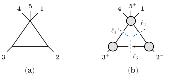
Figure 6: The triangle integral function ${\cal I}_{3}(k_{2},k_{3},K_{451})$ (left) and the associated triple cut (right). The virtual states in the loop are fixed to be a complex scalar. While the scalar integral coefficient turns out to vanish, some tensor coefficients are non-zero. The tensorial coefficients are important input for the computation of lower-point integral coefficients in the numerical unitarity approach.

We consider the amplitude $A^{s}_{5}(1^{-},2^{-},3^{+},4^{+},5^{+})$ with a scalar circulating in the loop. Amplitudes of this kind were first computed in refs. [22] using the unitarity method. Here we are only interested in the computation of a single triple-cut, as shown in fig. 6. It turns out that some tensor coefficients (26) are non-vanishing while the scalar triangle coefficient $c_{234}^{0}$ vanishes. This simple example allows to illustrate how to apply some of the methods that were introduced earlier.

In later parts of this review we will discuss further important aspects of such unitarity computations. In section 4.5 we will discuss, based on the present example, how to compute tensor coefficients numerically using discrete Fourier transformation, following the notation in [21]. Building on this, in section 4.6, we will explain how numerical precision can be monitored during computation of such triple-cuts.

We start with the computation of the triple cut fig. 6. A momentum parametrisation and reference momenta, similar to eq. (17), are given by,

$$n^{+}=\lambda_{2}\tilde{\lambda}_{3}\,,\quad n^{-}=\lambda_{3}\tilde{\lambda}_{2}\,,\quad n^{\pm}\cdot K_{i}=0\,,$$

$$\ell_{2}^{a}=\left(\lambda_{2}+t\lambda_{3}\right)\,\tilde{\lambda}_{2}\,,\quad\ell_{3}^{a}=t\,\lambda_{3}\,\tilde{\lambda}_{2}\,,\quad\ell_{4}^{a}=\lambda_{3}\,\left(-\tilde{\lambda}_{3}+t\tilde{\lambda}_{2}\right)\,.$$ (57)

This is a special case of solutions of the on-shell conditions for integrals with massless corners as explained below eq. (54). The on-shell momentum space takes the form of a light cone and consists of two parts, with the second branch, $\ell_{i}^{b}$, related to (57) by parity reflection $\lambda^{i}\leftrightarrow\tilde{\lambda}^{i}$. The loop momentum is then,

$$\ell_{2}^{b}=\lambda_{2}({\tilde{\lambda}}_{2}+t^{\prime}{\tilde{\lambda}}_{3})\,\quad\ell_{3}^{b}=t^{\prime}\,\lambda_{2}{\tilde{\lambda}}_{3}\,,\quad\ell_{4}^{b}=(-{\tilde{\lambda}}_{3}+t^{\prime}{\tilde{\lambda}}_{2}){\tilde{\lambda}}_{3}\,.$$ (58)

Notice that a more standard way to write the above parametrization would use $n^{1}=i(n^{+}+n^{-})/\sqrt{s_{23}}$, $n^{2}=(n^{+}-n^{-})/\sqrt{s_{23}}$ and $\ell_{3}^{a,b}=-t\sqrt{s_{23}}(in^{1}\pm n^{2})$. The use of complex momenta is crucial in order to evaluate such unitarity cuts.

The triple-cut, fig. 6, is given by the product of three tree amplitudes,

$$\hskip-28.45274pt\bar{c}_{234}(\ell_{i}) = A_{3}^{\rm tree}((-\ell_{2})^{s},2^{-},(\ell_{3})^{s})A_{3}^{\rm tree}((-\ell_{3})^{s},3^{+},\ell_{4}^{s})A_{5}^{\rm tree}((-\ell_{4})^{s},4^{+},5^{+},1^{-},\ell_{2}^{s})\,.$$ (59)

Inserting explicit tree amplitudes we then obtain,

$$\bar{c}_{234}(\ell_{i})=\frac{(-i)\left[3\,\ell_{4}\right]^{2}\left[3\,(-\ell_{3})\right]^{2}}{\left[3\,\ell_{4}\right]\left[\ell_{4}\,(-\ell_{3})\right]\left[(-\ell_{3})\,3\right]}\,\times$$

$$\frac{i\,{\left\langle(-\ell_{4})\,1\right\rangle}^{2}{\left\langle\ell_{2}\,1\right\rangle}^{2}}{\left\langle(-l_{4})\,4\right\rangle\left\langle 4\,5\right\rangle\left\langle 5\,1\right\rangle\left\langle 1\,\ell_{2}\right\rangle\left\langle\ell_{2}\,(-l_{4})\right\rangle}\times\frac{i\,{\left\langle(-\ell_{2})\,2\right\rangle}^{2}{\left\langle\ell_{3}\,2\right\rangle}^{2}}{\left\langle(-\ell_{2})\,2\right\rangle\left\langle 2\,\ell_{3}\right\rangle\left\langle\ell_{3}\,(-\ell_{2})\right\rangle}\,,$$ (60)

and after using the above momentum parametrisation, eq. (57),

$$\bar{c}_{234}(\ell_{i}^{a}) = -\frac{t^{2}\left\langle 1\,3\right\rangle^{2}\left[3\,2\right]\left(\left\langle 2\,1\right\rangle+t\,\left\langle 3\,1\right\rangle\right)}{\left\langle 3\,4\right\rangle\left\langle 4\,5\right\rangle\left\langle 5\,1\right\rangle}\,,$$

$$\bar{c}_{234}(\ell_{i}^{b})=0\,,$$ (61)

where the triple-cut vanishes on the second branch $\ell^{b}$ due to the vanishing of the three-point vertices for these momenta.

We can make several observations: (a) There is no term constant in $t$ consistent with the absence of scalar triangles [22]. (b) The maximal power of $t$ is three, consistent with the three powers of loop momentum expected from power-counting of a triangle diagram. (c) The expression (61) has no poles at finite non-zero values of $t$ consistent with the absence of scalar boxes for this particular combination of external helicities and scalar states in the loop [22]. The equations (51) thus simplify with box-subtraction terms being zero and, thus, absent.

The parametrization of the numerator tensors (3.3.3) is given by,

$$\bar{c}_{234}(\ell) = c^{3}\,(n^{+}\cdot\ell)^{3}+c^{2}\,(n^{+}\cdot\ell)^{2}+c^{1}\,(n^{+}\cdot\ell)+c^{0}+\,$$ (62)

$$c^{-1}(n^{-}\cdot\ell)+c^{-2}(n^{-}\cdot\ell)^{2}+c^{-3}(n^{-}\cdot\ell)^{3}\,.$$

The next step is to relate this parametrization of the numerator tensors (62) to the expressions for the triple cut eq. (61). For on-shell momenta we find for (62),

$$\bar{c}_{234}(\ell^{a}) = c^{3}\,(-s_{23}t)^{3}+c^{2}\,(-s_{23}t)^{2}+c^{1}\,(-s_{23}t)+c^{0}\,,$$

$$\bar{c}_{234}(\ell^{b}) = c^{0}+c^{-1}\,(-s_{23}t^{\prime})^{1}+c^{-2}\,(-s_{23}t^{\prime})^{2}+c^{-3}\,(-s_{23}t^{\prime})^{3}\,,$$ (63)

where any of the on-shell momenta $\ell^{a,b}_{i}$ $i=2,3$ or $4$, can be used.

Comparing the polynomials in $t$ and $t^{\prime}$ given by cut (61) and ansatz (63) we find all tensor coefficients,

$$c^{0}=0=c^{1}=c^{-i}\,,\quad c^{i\,\geq\,2}=-s_{23}\,A_{5}^{\rm tree}\left(\frac{\left\langle 3\,1\right\rangle}{\left\langle 2\,1\right\rangle}\right)^{i}\,.$$ (64)

In an analytic approach, it is of course no problem to compare the $t$-dependent expressions. What matters here, is that the tensor basis gives linearly independent functions on the solution space of $\ell^{a,b}$, so that all tensor coefficients can be identified. This will turn out sufficient for the related numerical approach, as we will discuss in section 4.5.

Thus, effectively by replacing $t\rightarrow-(n^{+}\cdot\ell_{2})/s_{23}$ in (61) we obtain the off-shell loop-momentum dependence,

$$\bar{c}_{234}(\ell)=-s_{23}\,A^{\rm tree}_{5}\,\left(\frac{(n^{+}\cdot\ell)\left\langle 3\,1\right\rangle}{\left\langle 2\,1\right\rangle}\right)^{2}\left(1+\frac{(n^{+}\cdot\ell)\left\langle 3\,1\right\rangle}{\left\langle 2\,1\right\rangle}\right)\,,$$ (65)

For the special case of this example, many coefficients including the scalar coefficient $c^{0}$ vanish. Because of this the associated triangle integral does not contribute to the given amplitude. The computation of the tensor coefficients is important, nevertheless, as they are used when computing the two-particle cuts, for which they serve as subtraction terms as apparent from eq. (51).

In the above analysis we relied on the fact that we had analytic expressions available. In the following section we will see that a purely numerical approach can be set up to follow very similar computational steps to obtain scalar and tensor coefficients.

4.5 Discrete Fourier Transform

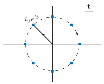
Figure 7: The discrete Fourier transformation to obtain integral coefficients. The triple cut contribution depends only on a small number of functions. Instead of a contour integral, the triple-cut may thus be evaluated on a discrete set of points. All scalar and tensor coefficients are obtained exactly in a numerical procedure.

We continue the discussion of the above example in section 4.4. A direct way to extract the tensor coefficients from the cut expression $\bar{c}_{234}(\ell_{i}^{a})$ in eq. (61) is through contour integrals,

$$c^{k}=\frac{1}{2\pi i}\int\frac{dt}{t}\left(\frac{t}{-s_{23}}\right)^{-k}\bar{c}_{234}(t)\,,$$ (66)

which take the form of a Fourier transformation in an angle $\phi$ for an integration contour $t=t_{0}e^{i\phi}$.

From a power-counting argument we know a priory that only a finite number of monomials in $t$ may appear. In particular, we know that $t$ will at most appear as a third power $t^{3}$. We may thus use a discrete version of the above contour integral fig. 7,

$$c^{k}=\frac{1}{m}\sum_{j=1}^{m}\left(\frac{t_{0}e^{2\pi i\,j/m}}{-s_{23}}\right)^{-k}\bar{c}_{234}(t=t_{0}e^{2\pi i\,j/m})\,,\quad\mbox{with}\quad m\geq 4\,,$$ (67)

giving an exact numerical way to obtain the required tensor coefficients. Typically the expected tensor-rank determines the number of points that need to be sampled in the above sum. For the example in section 4.4 four points, $m=4$ would be sufficient.

For the computation of all tensor coefficients in equations (26), (27) and (28) as well as in equations (88), (89), (90) and (91) analogous discrete sums can be constructed [21]. The central observation is that the numerator tensors are related to a finite number of functions. For phase-space integrals the orthogonality of these functions can be used to extract a particular tensor coefficient from a unitarity cut. For numerical approaches a related discrete versions of such integrals can be setup.

4.6 Numerical Stability

A clear understanding of the relation between numerator tensors and a function basis in phase-space can be further exploited; we can check the numerical precision during the computation of loop amplitudes.

Loss of precision may occur on a given phase-space point, for example, due to an unfortunate choice of reference momenta $n^{i}$ (17) or a vanishing Gram determinant (35). A particularly universal way to deal with loss of precision is the use of higher precision arithmetics [79]. As demonstrated in ref. [21], for an efficient approach one tries to identify the computational steps that lead to large round-off errors and then to re-evaluates only the problematic contributions to the amplitude (and only those terms) using higher-precision arithmetic. Use of higher precision arithmetics is more time consuming. Such an approach requires that results be sufficiently stable in the first place, so that the use of higher precision is infrequent enough to incur only a modest increase in the overall evaluation time; this is indeed the case.

The simplest test of numerical stability [79, 28, 21, 68, 38] is checking whether the known infrared singularity of a given matrix element has been reproduced correctly. Typically, a combination of various checks is required. A refined test [21] can be setup to check the accuracy of the vanishing of certain higher-rank tensor coefficients. From power-counting arguments we know on general grounds which high-rank tensor coefficients have to vanish. All tensors with rank greater than $m$ must vanish, for the $m$-point integrals with $m=2,3,4$. The central advantage of this check is that small parts of the computation may be singled out for re-computation, reducing the computation time accordingly.

For the above example of a triple cut computation, section 4.4, a check of the vanishing tensor coefficients may be implemented as an extension of the discrete Fourier sum. If a tensor of rank-four were to exist it could be computed numerically by,

$$c^{k=4}=\frac{1}{m}\sum_{j=1}^{m}\left(\frac{t_{0}e^{2\pi i\,j/m}}{-s_{23}}\right)^{-k}\bar{c}_{234}(t=t_{0}e^{2\pi i\,j/m})\,,\quad\mbox{with}\quad m\geq 5.$$ (68)

Clearly $c^{4}$ should always turn out to be zero, $c^{4}=0$. For finite precision the deviation of $c^{4}$ from zero can be used to monitor precision of the intermediate computational steps. This test requires to sample more values of the complex parameter $t$; $m=5$ instead of $m=4$. However, observing an instability at the level of an integral coefficient as opposed to a failing check of an infrared-pole has the big advantage, that one can recompute very targeted a small part (the specific triangle coefficient) of the full amplitude.

The parameters of such a rescue system have to be tuned in order to optimize efficiency. This includes the question which integral coefficients to check and what deviations from zero to expect for a given tensor coefficient. Some further details of this approach can be found, for example, in [21].

4.7 A Box Example.

Here we will discuss the pure gluon amplitude $A_{5}^{g}(1^{-},2^{-},3^{+},4^{+},5^{+})$. The analysis below will be purely analytic, however, in the way we set it up it is straightforward perform all computations numerically. Since this amplitude has five external massless legs, the box functions can have one external massive leg, and three massless ones. One of these box functions with massive legs $K_{12}=k_{1}+k_{2}$, is given by,

$${\cal I}(K_{12})=\hat{\mu}^{2\varepsilon}\int\frac{d^{4-2\varepsilon}\ell}{(2\pi)^{4-2\varepsilon}}\frac{1}{\ell^{2}(\ell-k_{1}-k_{2})^{2}(\ell-k_{1}-k_{2}-k_{3})^{2}(\ell+k_{5})^{2})}\,,$$

and displayed in fig. 8. The other boxes have the massive leg being $K_{23}$, $K_{34}$, $K_{45}$ or $K_{51}$.

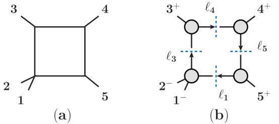
Figure 8: The box integral function ${\cal I}(K_{12})$ (left) and the associated quadruple cut (right). The helicity sum over internal states is suppressed in the graphic.

We focus here on the analysis of the coefficient of ${\cal I}(K_{12})$. The first step is to parametrize the integrand $\bar{d}_{1345}(\ell)$ in eq. (11) that extends the box function with a numerator tensor. The transverse momentum space (17) is one-dimensional and is spanned by a single vector $n^{1\,\mu}$,

$$n^{1}\cdot K_{12}=n^{1}\cdot k_{3}=n^{1}\cdot k_{4}=n^{1}\cdot k_{5}=0\,,$$ (69)

with the explicit solution for $n^{1\,\mu}$ given by,

$$n^{1}\cdot\ell\equiv([3|k_{4}k_{5}\ell|3\rangle-\langle 3|k_{4}k_{5}\ell|3])/s_{34}s_{45}\,,$$ (70)

where the loop momentum $\ell$ is identified with $\ell_{1}$ as defined in fig. 8. The only symmetric traceless tensor (20) in the transverse space is given by the vector $n^{1\,\mu}$ itself; $n^{\mu}=n^{1\,\mu}$ as in section 3.3.3. The numerator tensors of the box integrals are then parametrized as,

$$\frac{d^{0}_{1345}+d^{1}_{1345}\,(n^{1}\cdot\ell)}{\ell^{2}(\ell-k_{1}-k_{2})^{2}(\ell-k_{1}-k_{2}-k_{3})^{2}(\ell+k_{5})^{2})}\,,$$ (71)

resembling the generic form in eq. (26).

The coefficients $d^{1}_{1345}$ and $d^{0}_{1345}$ have to be determined by comparing the quadruple cut equation (51) to the ansatz (71) at the associated on-shell kinematics. In four dimensions the on-shell conditions,

$$\ell^{2} =0=(\ell-k_{5})^{2}=(\ell+k_{3})^{2}=(\ell+K_{34})^{2}\,,$$ (72)

have two solutions. A general form for the on-shell momenta can be found in ref. [21]. Explicitly, one set of on-shell momenta is given by,

solution (a): $$\ell_{5}=\frac{s_{23}}{\left[4|K_{12}|5\right\rangle}\lambda_{5}{\tilde{\lambda}}_{4}\,,\quad\ell_{1}=-\frac{\left\langle 3\,4\right\rangle}{\left[4|K_{12}|5\right\rangle}\lambda_{5}({{\raise 0.91666pt\hbox to9.20833pt{\hss/\hss}\hbox to0.0pt{\hss$K$}}}_{12}\lambda_{3})\,,$$ (73)

$$\ell_{3}=\frac{\left[3\,4\right]}{\left[4|K_{12}|5\right\rangle}\lambda_{3}({{\raise 0.91666pt\hbox to9.20833pt{\hss/\hss}\hbox to0.0pt{\hss$K$}}}_{12}\lambda_{5})\,,\quad\ell_{4}=\frac{\left[3|K_{12}|5\right\rangle}{\left[4|K_{12}|5\right\rangle}\lambda_{3}{\tilde{\lambda}}_{4}\,,$$

with the second set of on-shell momenta, solution (b), being related by parity conjugation; exchanging $\lambda_{i}\leftrightarrow\tilde{\lambda}_{i}$. We used here notation as discussed in eq. (32).

The quadruple cut is given by a product of four tree amplitudes summed over internal helicity states,

$$\hskip-28.45274pt\bar{d}_{1345}(\ell_{i}) = \sum_{h_{i}}A_{4}^{\rm tree}((-\ell_{2})^{-h_{2}},1^{-},2^{-},\ell_{3}^{h_{3}})A_{3}^{\rm tree}((-\ell_{3})^{-h_{3}},3^{+},\ell_{4}^{h_{4}})\times$$ (74)

$$\qquad\times A_{3}^{\rm tree}((-\ell_{4})^{-h_{4}},4^{+},\ell_{1}^{h_{1}})A_{3}^{\rm tree}((-\ell_{1})^{-h_{1}},5^{+},\ell_{2}^{h_{2}})\,.$$

Only the momenta in eq. (73) give a non-vanishing contribution to the quadruple-cut (74); for the internal helicities $\{h_{1},h_{2},h_{3},h_{4}\}=\{-,-,+,+\}$. In total we have,

$$\hskip-28.45274pt\mbox{solution (a):}\quad\bar{d}_{1345}(\ell_{i}) = \frac{\left\langle 1\,2\right\rangle^{3}}{\left\langle 2\,\ell_{3}\right\rangle\left\langle\ell_{3}\,(-\ell_{2})\right\rangle\left\langle(-\ell_{2})\,1\right\rangle}\frac{\left[3\,\ell_{4}\right]^{3}}{\left[\ell_{4}\,(-\ell_{3})\right]\left[(-\ell_{3})\,3\right]}\times$$

$$\quad\times\frac{\left\langle\ell_{1}\,(-\ell_{4})\right\rangle^{3}}{\left\langle 4\,\ell_{1}\right\rangle\left\langle(-\ell_{4})\,4\right\rangle}\frac{\left[(-\ell_{1})\,5\right]^{3}}{\left[5\,\ell_{2}\right]\left[\ell_{2}\,(-\ell_{1})\right]}$$

$$= is_{34}s_{45}\,A_{5}^{\rm tree}(1^{-},2^{-},3^{+},4^{+},5^{+})\,,$$

$$\hskip-28.45274pt\mbox{solution (b):}\quad\bar{d}_{1345}(\ell_{i}) = 0\,.$$ (75)

In order to determine the integral coefficients $d_{1345},d^{1}_{1345}$ we have to evaluate ansatz for the integral on the unitarity cut. For the particular momenta no other terms in the ansatz contribute leading terms in the factorization limit. We thus obtain,

$$\bar{d}_{1345}(\ell_{i}^{a,b})=d^{0}_{1345}+d^{1}_{1345}\,(n^{1}\cdot\ell_{i}^{a,b}) = d^{0}_{1345}\pm d^{1}_{1345}\,,$$ (76)

where any on-shell momentum $\ell_{i}$ may be used in the numerator tensor, due to the properties of the vector $n^{1\,\mu}$ as specified in eq. (70).

Using the values of the quadruple cut in eq. (75) we thus can solve for the unknowns $d^{0}_{1345}$ and $d^{1}_{1345}$,

$$d^{0}_{1345}=d^{1}_{1345}=\frac{i}{2}s_{34}s_{45}\,A_{5}^{\rm tree}(1^{-},2^{-},3^{+},4^{+},5^{+})\,.$$ (77)

That the integral coefficients $d^{0}_{1345}$ and $d^{1}_{1345}$ turn out to take identical values is a low point accident related to the presence of three-point amplitudes in the unitarity cut. For the value of the one-loop amplitude the tensorial term is of no immediate importance; it drops out after integration. However, for the computation of the remaining triangle and bubble coefficients this is an important ingredient.

The normalization factor $1/2$ in scalar integral coefficient (77) is usually attributed to an ’averaging over’ quadruple cut solutions [25]. In the presented computation this factor appears, somewhat differently, from inverting the set of linear equations (76).

4.8 Rational Terms From $D$-dimensional Unitarity Cuts

The rational terms (7) are free of branch cut singularities and cannot be detected by unitarity methods in four dimensions. Away from four dimensions, $D=4-2\epsilon$, rational terms carry factors of $(-s)^{-\epsilon}=(\hat{\mu})^{2\epsilon}(1-\epsilon\ln(-s/\hat{\mu}^{2})+{\cal O}(\epsilon^{2}))$, in order to compensate for the dimensionality of the coupling constant. The so introduced logarithms, in turn, make it possible to detect rational terms via $D$-dimensional unitarity methods [23] (see also the early work [129]). This version of unitarity, in which tree amplitudes are evaluated in $D$ dimensions, has been used in various analytic [72, 130] and numerical [29, 131, 124, 132, 79, 68, 133, 39, 70] studies. For a detailed discussion of analytic $D$-dimensional approaches we refer to [43]. Here we will follow the approach discussed in [29] including elements of [124].

4.8.1 Dimension Dependence.

The prescription of the $D$-dimensional unitarity method is to compute the $D$-dimensional loop-amplitudes and in the end take the limit, $D=4-2\epsilon$ with $\epsilon\rightarrow 0$. The combined dependence of integrals and their coefficients on the regulator $\epsilon$ yields the finite rational terms.

In numerical approaches the dependence on the dimension parameter $D$ is not as accessible as in an analytic approaches. Amplitudes may only be computed in a fixed dimension. The typical strategy, to deal with this issue, is to numerically compute in distinct discrete dimensions. With a clear understanding of the dimension dependence [29], the dimension parameter may be reinstated in the final steps of the computation. The limit $D\rightarrow 4$ is then performed analytically. We will discuss the $D$-dependence in detail in the following.

The origin of the $D$-dependence is twofold. While the external momenta and states are kept in four dimensions, polarization states and momenta in the loop are extended beyond four dimensions. The two sources for dependence on $D$ are the sums over virtual polarization states in $D$ dimensions and momentum invariants formed using $D$-dimensional loop momentum.

We consider first the dependence of rational terms on $D$-dimensional polarization states. A priori one would need to sum over the particle spectra of virtual gluons and fermions extended beyond four dimension. This can be done in practice [29], however, we will describe a shortcut, that avoids considering polarizations states beyond four dimensions altogether. Applying the arguments of section 3.5 we can relate the rational terms of QCD amplitudes with internal gluons and fermions to amplitudes with virtual scalar and fermionic states. The extension of scalar states to $D$-dimensions is straight forward as, in contrast to gluonic states, no additional polarizations have to be taken into account. In fact, it turns out that the $D$ dependence originating in the change of the number of polarization states with dimensionality my thus be avoided. Such an approach is computationally more efficient. The computation time grows faster than linearly with the number of particle states circulating in the loop. The computation of amplitudes of a complex scalar as opposed to (massless) vector particles leads to efficiency gains in $D>4$ dimensions.

For the computation of rational terms it is, thus, sufficient to consider simplified, yet generic amplitudes with:

1. closed scalar loops,

2. mixed scalar and fermion loops.

Even though QCD has no scalars, introducing them is a useful trick. For QCD like theories these assumptions are no restriction for the computation of rational terms; contributions from either only virtual gluons or fermions are related to virtual scalars (44). Similarly, rational terms from mixed gluon and fermion loops can be mapped to the ones with the gluon replaced by a scalar, see e.g. [78, 24]. Loops with mixed fermion and scalar states do only give rise to state sums over fermions which exit to external sources. Since for these amplitudes no closed loop of Dirac gamma matrices can be formed, no explicit dependence on the number of fermion states appears. We thus avoid the dependence on the dimensionality through the number of spin states.

The second source of the dimension dependence of loop amplitudes is the dependence on the $D$-dimensional loop momentum. This dependence is simplified due to the fact that we keep external polarizations and momenta in strictly four dimensions. Splitting the loop momentum into a four- and $(D-4)$-dimensional part, $\ell^{\mu}=\hat{\ell}^{\mu}+\tilde{\ell}^{\mu}$, the dependence on the $(D-4)$-dimensional part is limited to the form,

$$\mu^{2}=-(\tilde{\ell}\cdot\tilde{\ell})\,.$$ (78)

That is, no other vectors with non-vanishing components in $(D-4)$ are available to form scalar products and we ignore linear $\mu$-terms built from $\epsilon$-tensors. Rotation symmetry in the $(D-4)$-dimensional part of momentum space is preserved in this way.

4.8.2 The Loop Integrand.

The integrand basis has to include pentagon terms, when working in $D$-dimensions [29],

$$A^{{\rm 1\hbox{-}loop},D}_{n}(\ell) = \sum_{i_{1}<\ldots<i_{5}}\frac{\tilde{e}_{i_{1}i_{2}i_{3}i_{4}i_{5}}(\ell)}{D_{i_{1}}D_{i_{2}}D_{i_{3}}D_{i_{4}}D_{i_{5}}}+\sum_{i_{1}<i_{2}<i_{3}<i_{4}}\frac{\tilde{d}_{i_{1}i_{2}i_{3}i_{4}}(\ell)}{D_{i_{1}}D_{i_{2}}D_{i_{3}}D_{i_{4}}}$$ (79)

$$+\sum_{i_{1}<i_{2}<i_{3}}\frac{\tilde{c}_{i_{1}i_{2}i_{3}}(\ell)}{D_{i_{1}}D_{i_{2}}D_{i_{3}}}+\sum_{i_{1}<i_{2}}\frac{\tilde{b}_{i_{1}i_{2}}(\ell)}{D_{i_{1}}D_{i_{2}}}\,,$$

with propagators and numerators depending on the $D$-dimensional loop momentum $\ell^{\mu}=\hat{\ell}^{\mu}+\tilde{\ell}^{\mu}$. We suppressed the tadpole terms $a_{i_{1}}(\ell)$ which are not needed for computation of rational terms in amplitudes with only massless states. As compared to the earlier expression (11) the form of the numerator terms has to be adapted to the $D$-dimensional case as will be discussed in section 4.8.4. The generalization to massive states has been presented in [132].

The absence of terms with more than five propagators in eq. (79) is due to the restriction to strictly four dimensional external momenta and polarization vectors [115, 116]. (See also [117] for a recent discussion including generalizations to two-loop integrals.) Integrands with more than five propagators can be reduced to at least pentagon terms. At most five independent momentum vectors can be formed in $D$ dimensions, since the $(D-4)$-dimensional momentum $\tilde{\ell}^{\mu}$ is conserved in the loop. Because of this, Gram determinants which depend on the loop momentum and five or more independent momenta have to vanish. The resulting identities between momentum invariants can be used to reduce higher $n$-point propagator structures recursively to at least pentagon integrals.

4.8.3 $D$-dimensional Unitarity Relations.

As for the cut-containing parts, the computation of $D$-dimensional loop amplitudes amounts to determining the coefficients of a basis of scalar and tensor integrands and subsequently performing the loop integrations. A generalization of the unitarity relations (51) can be used to completely determine the loop integrand (79).

The restriction to purely four-dimensional external momenta has important implication for the unitarity cuts of the internal propagators. In fact, the $(D-4)$-dimensional component $\tilde{\ell}^{\mu}$ of the loop momentum is conserved and enters all propagators in the form of a mass term,

$$\frac{i}{(\ell-K_{i})^{2}}=\frac{i}{(\hat{\ell}-K_{i})^{2}-\mu^{2}}\,.$$ (80)

For unitarity cuts, this observation leads to an important restriction. In addition to the four momentum components of $\hat{\ell}^{\mu}$ we thus obtain only one additional degree of freedom, i.e. $\mu^{2}$. We can then put at most five propagators on shell, allowing us to consider at most penta cuts. Of course this meshes well with the absence of higher point functions in eq. (79) in the first place.

The unitarity relations are generalized to $D$ dimensions, by including an additional generalized penta cut,

$$\bar{e}_{i_{1}i_{2}i_{3}i_{4}i_{5}}(\ell) = \sum_{D\hbox{-}{\rm dim}\,\,{\rm states}}A_{n_{i_{1}}}^{\rm tree}(\ell)A_{n_{i_{2}}}^{\rm tree}(\ell)A_{n_{i_{3}}}^{\rm tree}(\ell)A_{n_{i_{4}}}^{\rm tree}(\ell)A_{n_{i_{5}}}^{\rm tree}(\ell)\,,$$ (81)

which is defined for appropriate on-shell loop momentum, $\ell$. The remaining unitarity cuts are implemented similar to the four-dimensional case (see eq. (51)), however, including additional subtraction terms from the pentagon-coefficients $\tilde{e}_{i_{1}i_{2}i_{3}i_{4}i_{5}}(\ell)$.

We may work in any discrete dimension bigger than four, which accounts for the full loop-momentum dependence in $D$ dimensions. The internal state sums have to be extended to the $D$ dimensional setup. For the case of a scalar state circulating in the loop, the $D$-dimensional extension of the scalar tree amplitudes is to be considered. Given the simple dependence (78) on the $(D-4)$-dimensional loop momentum it is sufficient to consider a scalar in five dimensions (see also [29]) to obtain the full dependence on $\mu^{2}$. Equivalently, one can consider four-dimensional virtual scalar states with a (dynamical) mass [23, 124].

Typically, the on-shell conditions do not constrain the loop momenta completely, but lead to a variety of solutions. Enforcing the unitarity relations (81) on the variety of on-shell solutions gives an infinite set of equations. We will discuss the parametrization of the $D$-dimensional numerator tensors below in section 4.8.4 and section 4.8.5 which allows to determine all needed integral coefficients.

4.8.4 Numerator Tensors.

In order to parametrize the numerator tensors of a given propagator structure in eq. (79) it is convenient to introduce an adapted vector basis in momentum space. The $D$-dimensional momentum space is split into three subspaces spanned by the vectors $K_{i}$, $n^{i}$ and $m^{i}$ [29],

$$K_{i}\quad\mbox{for}\quad i\in\{1,\cdots,n-1\}\,,$$

$$n^{i}\quad\mbox{for}\quad i\in\{1,\cdots,4-(n-1)\}\,\qquad m^{i}\quad\mbox{for}\quad i\in\{5,\cdots,D\}\,$$ (82)

$$(n^{i},n^{j})=\delta^{ij}\,,\quad(m^{i},m^{j})=\delta^{ij}\,,\quad(n^{i},m^{j})=0\,,\quad(n^{i},K_{j})=0\,,$$

$$g^{\mu\nu}_{\perp}\equiv\sum_{i=1}^{4-(n+1)}n^{i\mu}n^{i\nu}\,,\quad g^{\mu\nu}_{D-4}\equiv\sum_{i=5}^{D}m^{i\mu}m^{i\nu}\,.$$ (83)

In a first step, the $D$-dimensional space is split into two subspaces: the $4$-dimensional subspace and its $(D-4)$-dimensional complement, ${m^{i}}$. In a second step, the $4$-dimensional momentum space is further decomposed into a physical space, spanned by the independent external momenta of the integral $K_{i}$ and their transverse space within four dimensions, $\{n^{i}\}$. For convenience the bases $\{n^{i}\}$ and $\{m^{i}\}$ are orthonormal. The metrics $g^{\mu\nu}_{\perp}$ and $g^{\mu\nu}_{D-4}$ are projections of $g_{\mu\nu}$ to the respective subspaces.

We can follow similar steps as in section 3.3.2 to conclude that the generic numerator tensors are traceless symmetric tensors in the whole of the transverse space,

$$n_{\mu_{1}\cdots\mu_{k}}=n^{i_{1}}_{\{\mu_{1}}\cdots n^{i_{l}}_{\mu_{l}}m^{j_{1}}_{\mu_{l+1}}\cdots m^{j_{k}}_{\mu_{k}\}}\,,$$

$$n_{\mu_{1}\mu_{2}\cdots\mu_{k}}g_{\perp}^{\mu_{1}\mu_{2}}+n_{\mu_{1}\mu_{2}\cdots\mu_{k}}g_{D-4}^{\mu_{1}\mu_{2}}=0\,,$$ (84)

where the curly-brackets indicate symmetrization and subtraction of all traces. More explicitly, the traces should be subtracted in transverse space, using the metrics $g_{\perp}^{\mu\nu}$ and $g_{D-4}^{\mu\nu}$, but not $g^{\mu\nu}$. Due to the rotation invariance in $(D-4)$ dimensions, the dependence on the $m^{i}$ is further restricted to appear solely in terms of $g^{\mu\nu}_{D-4}=\sum_{i=5}^{D}m^{i\mu}m^{i\nu}$.

A subtlety appears here for numerical applications; the traceless-condition introduced a dependence on the dimensionality of space time, as illustrated by the following example,

$$n_{\mu\nu}=\sum_{i=5}^{D}m^{i}_{\{\mu}m^{i}_{\nu\}}=\biggl{(}(g_{D-4})_{\mu\nu}-\frac{D-4}{4-(n+1)}\,(g_{\perp})_{\mu\nu}\biggr{)}\,,$$ (85)

yielding a $D$-dependent coefficient of $g_{\perp}^{\mu\nu}$ and thus an explicit $D$-dependence. For numerical computations we would like to avoid specifying $D$ and keep it as a parameter. Without loss of generality, the dependence on the space-time dimensionality can be tracked more conveniently by allowing terms with non-vanishing traces. This can be achieved at the minor cost of introducing terms that do not integrate to zero, section 4.8.6. In particular, as given in [29] we use instead a representation of the numerator tensors in terms of tensors that are trace-free only in the physical transverse space,

$$n_{\mu_{1}\cdots\mu_{k}}=n^{i_{1}}_{\{\mu_{1}}\cdots n^{i_{l}}_{\mu_{l}\}}g^{D-4}_{\mu_{l+1}\mu_{l+2}}\cdots g^{D-4}_{\mu_{k-1}\mu_{k}}\,,\qquad n_{\mu_{1}\mu_{2}\cdots\mu_{k}}g_{\perp}^{\mu_{1}\mu_{2}}=0\,,$$ (86)

The above rank-two tensor (85) would then be given by,

$$n_{\mu\nu}\ell^{\mu}\ell^{\nu}=(g_{D-4})_{\mu\nu}\ell^{\mu}\ell^{\nu}=-\mu^{2}\,,$$ (87)

without explicit dependence on the parameter $D$.

4.8.5 Tensor Basis.

An explicit form of the numerator tensors was given in [29]. The pentagon numerator tensors are,

$$\tilde{e}_{i_{1}i_{2}i_{3}i_{4}i_{5}}(\ell) = e^{0}_{i_{1}i_{2}i_{3}i_{4}i_{5}}\,,$$ (88)

where the absence of any loop-momentum dependence has to be noted. For this case the transverse space coincides with the $(D-4)$ dimensional space and no traceless tensor can be formed. Therefore terms of the form $\mu^{2}$ can be converted into inverse propagators and scalar terms and are represented by lower-point integrals and the scalar pentagon.

The remaining numerator tensors are, for the box,

$$\tilde{d}_{i_{1}i_{2}i_{3}i_{4}}(\ell) = \bar{d}_{i_{1}i_{2}i_{3}i_{4}}(\ell)+\mu^{2}(d^{2}_{i_{1}i_{2}i_{3}i_{4}}+d^{3}_{i_{1}i_{2}i_{3}i_{4}}t_{1})+\mu^{4}\,d^{4}_{i_{1}i_{2}i_{3}i_{4}},$$ (89)

for the triangles,

$$\tilde{c}_{i_{1}i_{2}i_{3}}(\ell) = \bar{c}_{i_{1}i_{2}i_{3}}(\ell)+\mu^{2}\left(c^{7}_{i_{1}i_{2}i_{3}}t_{1}+c^{8}_{i_{1}i_{2}i_{3}}t_{2}+c^{9}_{i_{1}i_{2}i_{3}}\right),$$ (90)

and finally for bubble coefficients they are,

$$\tilde{b}_{i_{1}i_{2}}(\ell) = \bar{b}_{i_{1}i_{2}}(\ell)+\mu^{2}b^{9}_{i_{1}i_{2}}.$$ (91)

Here the vectors we introduced $t_{i}=(n^{i}\cdot\ell)$. The $n^{i}$ are defined for each propagator structure of (79) individually as defined in eq. (83). The tadpole contributions may be found in the original literature. The $\mu$-independent tensors take the same form as given earlier, being traceless symmetric tensors in the vectors $n^{i}$. These tensorial structures parametrize the most generic tensor integrals, subject only to power-counting requirements of QCD like theories as well as the constraints from rotational symmetry manifest in dimensional regularization.

4.8.6 Integration.

The final step to extract the $D$-dimensional amplitude is to evaluate the integrals. We are interested here only in the computation of the rational terms. Only the new integrand structures of eqs. (88), (89), (90) and (91), proportional to powers of $\mu$ may contribute to the rational remainder in eq. (8).

As above terms dependent on vectors $n^{i}$ integrate to zero due to their angular dependence and can be dropped. In order to obtain the rational contributions we are left with terms proportional only to powers of $\mu^{2}$. Without spelling out the details, the non-vanishing limits are given by [134, 23, 124],

$$\lim_{D\rightarrow 4}\quad\int\frac{d^{D}\ell}{i\pi^{D/2}}\frac{\mu^{4}}{D_{i_{1}}D_{i_{2}}D_{i_{3}}D_{i_{4}}} = -\frac{1}{6}\,,\quad\lim_{D\rightarrow 4}\quad\int\frac{d^{D}\ell}{i\pi^{D/2}}\frac{\mu^{2}}{D_{i_{1}}D_{i_{2}}D_{i_{3}}}=-\frac{1}{2}\,,$$

$$\lim_{D\rightarrow 4}\quad\int\frac{d^{D}\ell}{i\pi^{D/2}}\frac{\mu^{2}}{D_{i_{1}}D_{i_{2}}} = -\frac{1}{6}\,K_{i_{1}}^{2},$$ (92)

The limits of these integrals combined with the associated integral coefficients add up to the rational term of the one-loop amplitudes. The rational term is then given by [130, 131, 29],

$$R_{n} = -\sum_{i_{1}<i_{2}<i_{3}<i_{4}}\frac{d_{i_{1}i_{2}i_{3}i_{4}}^{4}}{6}-\sum_{i_{1}<i_{2}<i_{3}}\frac{c_{i_{1}i_{2}i_{3}}^{9}}{2}-\sum_{i_{1}<i_{2}}\frac{K_{i_{1}}^{2}\,\,b_{i_{1}i_{2}}^{9}}{6}\,.$$ (93)

We note that the $D$-dimensional approach is very general and can be applied to higher loop computations. For evaluation of scheme shift and order $\epsilon$ contributions we refer to [29].

5 On-shell Recursion

On-shell recursions [47] rely on on-shell scattering amplitudes with a fixed number of partons in order to obtain the ones with arbitrary multiplicity. The underlying structures used in this approach are universal factorization and analyticity properties.

In fact, when intermediate states are nearly on-shell, amplitudes factorize into products of lower-point amplitudes. At tree-level, the naive attempt to invert factorization equations and assemble the on-shell factorized amplitudes into their parent amplitude raises two central questions: Firstly, how to recover the full off-shell kinematics away from the factorization limit? And, secondly, how to combine various factorization channels while avoiding double-counting? On-shell recursion was introduced by Britto, Cachazo, Feng and Witten [47]. These naive obstructions are overcome by the effective use of complex kinematics and the use of Cauchy’s residue theorem.

While originally constructed for tree amplitudes on-shell recursions can be extended to loop-level [19, 67, 20]. Compared to tree amplitudes, the obvious difficulty is that loop amplitudes contain branch cuts, which complicate the use of Cauchy’s theorem. The resolution to these difficulties has been to work on subparts of the amplitudes, which are purely rational functions. The price to pay is that additional, un-physical singularities have to be dealt with, which are present in subparts but cancel once the full amplitude is assembled. Un-physical poles can typically be understood from complementary information. In the case of on-shell recursions for rational terms spurious singularities are characterized using prior knowledge of the logarithmic parts of the amplitude. In addition, while factorization of loop amplitudes is understood for real kinematics, presently there are no theorems on the factorization properties of loop amplitudes with complex momenta. Indeed, there is a class of poles, ’unreal poles’  [19], whose contributions have to be taken into account and whose nature is not yet fully understood. For most applications unreal poles can be avoided using alternative factorization channels. (See, however, ref. [135] for recent progress with understanding the origin of unreal poles.)

Most recent developments focus on recursion relations at the integrand level [136] and have already led to many results in maximally supersymmetric Yang-Mills theory. Here we are mainly interested in on-shell recursions for loop amplitudes, which can be applied after integration has been performed.

For numerical applications at tree-level, on-shell recursions are efficient, allowing to repeatedly take advantage of the remarkable simplicity of the physical scattering amplitudes (e.g. Parke-Taylor amplitudes). At loop-level, on-shell recursions hold the potential of an efficient complement to unitarity approaches for two reasons: (a) Recursions can sidestep the computation of tensors coefficients (11) and deal entirely with the much smaller set of scalar integral coefficients. (b) On-shell recursions for rational terms rely on strictly four dimensional information and, thus, do not require more involved $D$-dimensional objects. Despite the potential of loop recursions, unitarity approaches are very universal and straightforward to implement for a large class of theories explaining their widespread use. The BlackHat-library [21], for example, makes use of both approaches and like this improves the efficiency of computations.

We will first point out some central ideas of on-shell recursions at tree-level and will then turn to loop-level recursion.

5.1 Tree Recursion

For a more complete discussion on tree level recursions we refer the reader to the chapter of the present review dedicated to this subject by Brandhuber, Spence and Travaglini [53]. Here we will merely introduce basic notation needed for the discussion of loop-level on-shell recursions.

On-shell recursion relations systematically construct a scattering amplitude (or parts of it) from its poles and residues in momentum space. Typically, a parametrization of the complexified phase-space in terms of a complex parameter $z$ is introduced. An amplitude $A_{n}(z)=A_{n}(\{k_{i}(z)\})$ is then reconstructed as the unique function with consistent poles and residues in the $z$-plane. Analyticity is in many cases so restrictive for the form of the amplitudes, that this is in fact possible. Prior knowledge of singularities in phase-space as well as a simple physical interpretation is a necessary input in this procedure.

A particularly useful parametrization of a plane in complexified phase-space is given in terms of a deformation of two momentum vectors [47],

$$A_{n}(z)\ =\ A_{n}(k_{1},\ldots,k_{j}(z),k_{j+1},\ldots,k_{l}(z),\ldots,k_{n}).$$ (94)

The momenta $k_{i}(z)$ are chosen to keep momenta on-shell and the overall momentum conservation intact. The explicit form of such a parametrization, denoted by ${[j,l\rangle}$, is given by the linear transformation,

$${[j,l\rangle}:\quad{\tilde{\lambda}}_{j}\rightarrow{\tilde{\lambda}}_{j}-z{\tilde{\lambda}}_{l}\,,\quad\quad\lambda_{l}\rightarrow\lambda_{l}+z\lambda_{j}\,,$$ (95)

where $z$ is a complex parameter. This shift of spinors leaves untouched $\lambda_{j}$, ${\tilde{\lambda}}_{l}$, and the spinors for all the other particles in the process. The corresponding momenta are,

$$k_{j}(z)=k_{j}-z\,\lambda_{j}{\tilde{\lambda}}_{l}\,,\qquad k_{l}(z)=k_{l}+z\,\lambda_{j}{\tilde{\lambda}}_{l}\,,$$ (96)

and on-shell conditions, here $k_{j}^{2}(z)=0=k_{l}^{2}(z)$, as well as overall momentum conservation remain intact, due to $k_{j}(z)+k_{l}(z)=k_{j}+k_{l}$.

Poles in the variable $z$ appear through propagators when intermediate momenta go on-shell,

$$\frac{i}{K^{2}_{\alpha}(z)}=\frac{i}{K_{\alpha}^{2}+z\left[l|K_{\alpha}|j\right\rangle}\,,$$ (97)

where $\alpha$ denoted a range of momentum vectors that contain momentum $k_{l}$ but not $k_{j}$. The location of the pole is given by $z_{\alpha}=-K_{\alpha}^{2}/\left[l|K_{\alpha}|j\right\rangle$. Near the singularity of the propagator (97), the amplitude is given by its factorization properties,

$$\lim\limits_{z\rightarrow z_{\alpha}}A_{n}(z)=\sum_{h}A^{h}_{\alpha,L}(z_{\alpha}){i\over K_{\alpha}^{2}+z\left[l|K_{\alpha}|j\right\rangle}A^{-h}_{\alpha,R}(z_{\alpha})\,,$$ (98)

and uniquely defines the residue on the pole in terms of the on-shell lower-point amplitudes $A^{h}_{\alpha,L}(z_{\alpha})$ and $A^{-h}_{\alpha,R}(z_{\alpha})$.

By using Cauchy’s residue theorem we can relate the amplitude at $z\!=\!0$, $A_{n}(0)$, to its poles. For a vanishing contour integral that encloses the point $z=0$, we find,

$$0=\oint_{\cal C}\frac{dz}{2\pi i}\frac{A_{n}(z)}{z}\,\quad\rightarrow\quad A_{n}(0)=-\sum_{{\rm poles}\,\,\alpha}{\rm Res}_{z=z_{\alpha}}\frac{A_{n}(z)}{z}.$$ (99)

The vanishing contour is associated to large complex momenta. In this region power-counting arguments can be used to show the vanishing of the function $A_{n}(z\rightarrow\infty)=0$. One may also include the residue at $z=\infty$. However, this residue is not related to a factorization limit as above (98) and has to be obtained by other means (see e.g. [67]).

When there is no large-$z$ contribution, the physical amplitude $A_{n}(0)$ is obtained explicitly by,

$$A_{n}(0)=\sum_{\alpha}\sum_{h}A^{h}_{\alpha,L}(z_{\alpha}){i\over K^{2}_{\alpha}}A^{-h}_{\alpha,R}(z_{\alpha})\,.$$ (100)

The on-shell amplitudes with fewer legs, $A_{\alpha,L}^{h}$ and $A_{\alpha,R}^{-h}$, are evaluated in kinematics that have been shifted by eq. (95) with $k_{i}(z_{\alpha})$, such that their intermediate momentum is on-shell, $K_{\alpha}(z_{\alpha})^{2}=0\,$ where $z_{\alpha}=-K^{2}_{\alpha}/\left[l|K_{\alpha}|j\right\rangle\,$.

The $n$-point amplitude $A_{n}$ is thus expressed in terms of sums over on-shell, but complex continued, amplitudes with fewer legs. These recursion relations can be extended to massive QCD, more general other theories and beyond four dimensional applications [137, 138]. Moreover, for certain helicity configurations, they lead to new all-multiplicity expressions for these amplitudes [139].

5.2 Recursion for Loop Amplitudes

On-shell recursion have been generalized to loop-level in refs. [19, 67, 20]. Following a similar strategy as outlined in section 5.1 for tree amplitudes, loop amplitudes are analyzed as functions of a complex parameter $z$. When applying a shift (95), we obtain,

$$A_{n}^{\rm 1\hbox{-}loop}(z)=\Bigl{[}C_{n}(z)+R_{n}(z)\Bigr{]}\,.$$ (101)

where $C_{n}(z)$ denotes the logarithmic part of the amplitudes, and $R_{n}(z)$ the rational remainders (8). In contrast to tree amplitudes, loop amplitudes (101) typically have branch cut singularities in the variable $z$ originating from the logarithms within $C_{n}(z)$.

The way we deal with branch cut singularities is to focus on subparts of the amplitude which are free of logarithms:

1. the rational remainder: $R_{n}(z)$

2. the integral coefficients: $d^{0}_{i}(z)$, $c^{0}_{j}(z)$ or $b^{0}_{k}(z)$ within $C_{n}(z)$

3. $D$-dimensional coefficients: $e^{0}_{h}(z)$, $d^{0}_{i}(z)$, $c^{0}_{j}(z)$, $b^{0}_{k}(z)$ or $a^{0}_{l}(z)$.

These integral coefficients are introduced in sections 3.3.3 and 4.8.5, respectively. These terms can be shown to inherit factorization properties on physical poles from universal factorization relations at loop-level. For an intermediate propagator going on-shell there are typically three contributions for each internal state,

$$\lim\limits_{K^{2}\rightarrow 0}A_{n}^{\rm 1\hbox{-}loop}=A_{L}^{\rm tree}\,{i\over K^{2}}\,A_{R}^{\rm 1\hbox{-}loop}+A_{L}^{\rm 1\hbox{-}loop}\,{i\over K^{2}}\,A_{R}^{\rm tree}+A_{L}^{\rm tree}\,{i\,{\cal F}\over K^{2}}\,A_{R}^{\rm tree}\,.$$ (102)

In the first two terms, one of the factorized amplitudes is a one-loop amplitude and the other is a tree amplitude. The last term will appear here simply as a one-loop correction to the propagator. (For details about subtleties of the ’factorization function’ ${\cal F}$ in massless theories we refer to [140].)

When considering subparts of the full amplitude, additional singularities, called spurious singularities, may appear. These singularities naturally cancel out in the full amplitude. A method to compute contributions from spurious singularities to rational terms $R_{n}$ will be discussed in section 5.3.2.

5.3 Recursions for the Rational Part.

The terms $R_{n}$ (8), which are purely rational in the spinor variables, cannot be computed using four-dimensional unitarity methods. On-shell recursion, however, allows us to construct these terms from purely four-dimensional data. Typically the information contained in the recursion relation has to be completed with properties of the cut part.

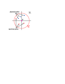
Figure 9: Using Cauchy’s theorem, rational expressions in loop amplitudes can be reconstructed from residues at poles in the complex plane. The poles are of two types: physical and spurious. All pole locations are known a priori. Residues at physical poles are obtained from universal factorization relations (102). Residues at spurious poles are obtained from the cut parts.
Reprinted fig. 9 with permission from [21] p.16. Copyright (2008) by the American Physical Society.

The central input for this approach is the detailed understanding of $R_{n}(z)$ as a function of $z$; we need to know the location of poles, their residues and an integration contour, along which $R_{n}(z)$ vanishes. Poles in the rational terms $R_{n}(z)$ may be grouped into two classes as shown in fig. 9: physical and spurious. The physical poles are present in the full amplitude $A_{n}(z)$, and correspond to genuine, physical factorization singularities. The spurious poles are not poles of $A_{n}(z)$ and cancel between the cut parts $C_{n}(z)$ and rational remainders $R_{n}(z)$. They originate from the presence of tensor integrals in the underlying field-theory representation of the amplitude, and appear as Gram determinant denominators (35). In unitarity approaches, inverse Gram determinants enter integral coefficients through on-shell loop-momentum parametrization. The exponent of the inverse Gram determinant in integral coefficients can be bounded by power-counting arguments. These denominators give rise to spurious singularities in individual terms.

An example for the appearance of Gram determinants in unitarity approach can be seen in the quadruple-cut computation in section 4.7. The Gram determinant (see also [21]),

$$\Delta(K_{12},k_{3},k_{4},k_{5})=2s_{45}\left\langle 4|K_{12}|5\right]\left[4|K_{12}|5\right\rangle\,,$$ (103)

appears in the on-shell loop momenta (73), through the factor $1/\left[4|K_{12}|5\right\rangle$; the remaining invariants cancel. The second factor, $1/\left[5|K_{12}|4\right\rangle$, appears in the parity conjugate on-shell momenta. This ’chiral’ dependence on inverse Gram determinants is typical for unitarity cuts with massless corners. In this particular example, the dependence on the Gram determinant (103) cancels in the final form of the integral coefficients in eq. (77). For the helicity configurations discussed the integral coefficients are the same as in maximally supersymmetric Yang-Mills and thus are effectively supersymmetric. Supersymmetric cancellations then reduce the naive power-count of loop momenta from four to zero, such that no dependence on Gram determinant remains in the integral coefficient. Explicit dependence of box-integrals on Gram determinant singularities can be found for example in analytic expressions in ref. [141].

Separating the different contributions of the shifted amplitude (101), we may write,

$$R_{n}(z)=R^{D}_{n}(z)+R^{S}_{n}(z)+R^{{\rm large}\ z}_{n}(z)\,,$$ (104)

where $R^{D}_{n}(z)$ contains all contributions from physical poles, $R^{S}_{n}(z)$ the contributions from spurious poles, and $R^{{\rm large}\ z}_{n}(z)$ the possible contributions from large deformation parameter $z$, if $R_{n}(z)$ does not vanish there. More explicitly, the rational terms can be expressed in terms of a partial fraction decomposition in $z$,

$$R_{n}^{D}(z)=\sum_{\alpha}{A_{\alpha}\over z-z_{\alpha}}\,,\qquad R^{{\rm large}\ z}_{n}(z)=\sum_{\sigma=0}^{\sigma_{\rm max}}D_{\sigma}z^{\sigma}\,,$$

$$R^{S}_{n}(z)=\sum_{\beta}\Biggl{(}{B_{\beta}\over(z-z_{\beta})^{2}}+{C_{\beta}\over z-z_{\beta}}\Biggr{)}\,,$$ (105)

where the coefficients $A_{\alpha},B_{\beta},C_{\beta},D_{\sigma}$ are functions of the external momenta. The poles in $z$ in eq. (105) are shown in fig. 9. The physical poles labeled by $\alpha$ are generically single poles. In general, in a renormalizable gauge theory, the spurious poles, labeled by $\beta$, may be either single or double poles. If $R_{n}(z)$ vanishes for large $z$, the $D_{\sigma}$ are all zero. If not, then $D_{0}$ gives a contribution to the physical rational terms, $R_{n}(0)$.

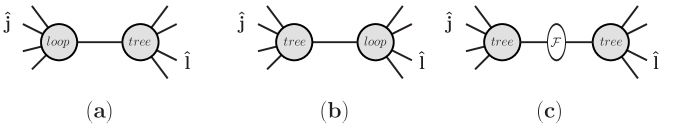
Figure 10: Diagrammatic contributions to on-shell recursion at one-loop for a $[j,l\rangle$ shift. The labels ’loop’ and ’tree’ refer respectively to (lower-point) tree amplitudes $A^{\rm tree}$ and rational remainders of one-loop amplitudes $R$. The central blob in (c) is the rational part of a one-loop factorization function ${\cal F}$ [140].

5.3.1 Physical Residues.

The contributions of the physical poles may be obtained efficiently using the on-shell recursive terms represented by the diagrams in fig. 10. The ’vertices’ labeled by ’tree’ denote tree-level on-shell amplitudes $A_{m}^{\rm tree}$, while the loop vertices ’loop’ are the rational remainders of on-shell (lower-point) one-loop amplitudes $R_{m}$, $m<n$, as defined in eq. (7). The contribution in fig. 10(c) involves the rational part of the additional factorization function ${\cal F}$ [140]. It only appears in multi-particle channels, and only if the tree amplitude contains a pole in that channel. Each diagram is associated with a physical pole (97) in the $z$ plane, as in fig. 9, and is computed similarly to the recursive diagrams at tree-level (100). Further details for the computation of the recursive diagrams in fig. 10 has been described in refs. [19, 143, 111].

5.3.2 Spurious Residues.

One approach to compute spurious residues is to use a completion of the integral functions, so called ’cut-completion’ [19, 67]. To this end, the integral basis is adjusted to subtract off spurious poles within their integral coefficients. This in turn moves all spurious poles from the rational part $R_{n}$ in (101) to the cut part $C_{n}$, such that the redefined rational remainder has poles only at the position of physical factorization singularities. The coefficients $B_{\beta}$ and $C_{\beta}$ vanish in this approach. Attention has to be paid to the factorization equation which will mix cut part and rational part non-trivially. This approach has led to the computation of the rational terms for a variety of one-loop MHV amplitudes with an arbitrary number of external legs [19, 67], as well as for six-point amplitudes.

For the purposes of a numerical program, however, it is simpler to extract the spurious residues from the known cut parts [21]. These residues, being absent in the full loop amplitude, are guaranteed to be the negatives of the spurious-pole residues in the rational remainder. That is, the spurious contributions are,

$$\lim\limits_{z\rightarrow z_{\beta}}C_{n}(z)=-\Biggl{(}{B_{\beta}\over(z-z_{\beta})^{2}}+{C_{\beta}\over z-z_{\beta}}\Biggr{)}+{\cal O}(z)\,,$$ (106)

where $C_{n}(z)$ is the shifted cut part appearing in eq. (7). Terms containing logarithms in the kinematic invariants cancel, but may as well be ignored for simplicity. The spurious poles at $z_{\beta}$ correspond to the vanishing of shifted Gram determinants, $\Delta_{m}(z_{\beta})=0$ for $m=3,4$, associated with triangle and box integrals.

In order to compute the rational parts $R_{n}$ we need to extract all residues $B_{\beta}$ and $C_{\beta}$ from the cut pieces $C_{n}(z)$. For this we evaluate the integral coefficients $d_{i}(z),c_{j}(z)$ and $b_{k}(z)$ numerically for complex, shifted momenta in the vicinity of the spurious pole. We also need to evaluate the loop integrals. This is done after using as input analytic series expansions of the integrals around vanishing Gram determinants,

$${\cal I}_{i}(z) \buildrel z\rightarrow z_{\beta}\over{\longrightarrow} {\cal I}_{i}^{\beta}(z)+\mbox{logarithms}\,$$

$${\cal I}_{i}^{\beta}(z) \,\,= \!\!(z-z_{\beta})^{k}\Bigl{(}\rho_{1}+(z-z_{\beta})\rho_{2}+\ldots\Bigr{)}\,.$$ (107)

The coefficients $\rho_{l}$ are rational functions in the kinematic variables which take a universal form. Examples of this procedure may be found in [21] with further details for generating these expansions using a dimension-shifting formula [144] may be found in [145]. It is important to have a precomputed analytic expansion available, as the logarithmic terms have to be dropped by hand; these terms do not cancel spurious poles in rational terms, but rather cancel between different integral functions. Thus we may avoid computing any logarithms or polylogarithms at complex momentum values. The expression obtained by replacing $C_{n}(z)$ according to these rules, in the vicinity of $z_{\beta}$, will be denoted by $C_{n}^{\beta}(z)$.

5.3.3 Discrete Fourier Sum for Spurious Residues.

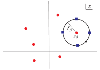
Figure 11: We obtain the residue at the spurious pole located at $z=z_{\beta}$ in the complex $z$ plane by a discrete Fourier sum, evaluating $C_{n}^{\beta}(z)$ on the (blue) squares on the circle of radius $\delta_{\beta}$ centered on $z_{\beta}$. The locations of other poles are represented by (red) dots. We ensure that $\delta_{\beta}$ is sufficiently small so that other poles give a negligible contribution to the residue.
Reprinted fig. 11 with permission from [21] p.22. Copyright (2008) by the American Physical Society.

The spurious-pole residues can be extracted from the cut parts by using a discrete Fourier sum. We evaluate $C_{n}^{\beta}(z)$ at $m$ points equally spaced around a circle of radius $\delta_{\beta}$ in the $z$ plane, centered on the pole location $z_{\beta}$, as depicted in fig. 11; i.e., $z=z_{\beta}+\delta_{\beta}e^{2\pi ij/m}$, for $j=1,2,\ldots,m$.

We can extract the coefficients $B_{\beta}$ and $C_{\beta}$ in eq. (105) via,

$$B_{\beta} \simeq -{1\over m}\sum_{j=1}^{m}\Bigl{[}\delta_{\beta}\,e^{2\pi ij/m}\Bigr{]}^{2}C_{n}^{\beta}(z_{\beta}+\delta_{\beta}e^{2\pi ij/m})\,,$$

$$C_{\beta} \simeq -{1\over m}\sum_{j=1}^{m}\delta_{\beta}\,e^{2\pi ij/m}\,C_{n}^{\beta}(z_{\beta}+\delta_{\beta}e^{2\pi ij/m})\,.$$ (108)

Both $m$, the number of evaluations, and $\delta_{\beta}$ are adjusted to optimize efficiency and numerical precisions. In general, an increase in $m$ increases the precision, but at the cost of computation time. We choose $\delta_{\beta}$ to be much smaller than the distance to nearby poles, but not so small as to lose numerical precision.

5.4 Recursion Relations for Integral Coefficients

Here we address the question of whether we can also apply recursion relations to the cut containing pieces $C_{n}(z)$. In fact it has been shown in [20] that it is possible to construct recursions, not for the full amplitudes, but in certain cases for the rational coefficients of the integrals. Such recursions can have important implication for the computation of rational terms, as we will discuss below in section 5.5.

With unitarity methods available, one of the central motivations for coefficient recursion are efficiency gains and insights for the recursive computation of rational terms. Rational recursion relies on the data from cut containing terms; the residues of Gram determinant poles. Gram determinant singularities are tied to their associated integral coefficients. A direct recursive approach to compute integral coefficients directly gives access to spurious residues of Gram determinant poles.

A firm grasp of the analytic properties of the integral coefficients is required. These properties differ from those of full amplitudes; in general these coefficients, being subparts of the full amplitude, contain physical poles as well as spurious poles of their own. Very much like for the case of rational terms, spurious poles originate from reduction of higher point tensor integrals and are associated to Gram determinant denominators.

The spurious poles are harder to deal with in a purely recursive way. An intricate web of cancellations between distinct integral coefficients guided by the integral functions leads to the cancellation of spurious poles between various logarithmic terms. Here, we do not want to disentangle the implicit consistency conditions. Rather, with an understanding of which spurious poles appear in which integral coefficient, we try to maneuver around them. A detailed discussion of the factorisation properties of one-loop amplitudes, as well the spurious singularities that appear, may be found in refs. [22, 140].

The factorisation of amplitudes follows from the combined behaviour of integral functions and the integral coefficients in the factorisation limit. If we turn this around, given the general factorisation (102) of an amplitude and given factorization properties of integral functions [22, 140], we may then determine the factorisation properties of the integral coefficients. By applying this logic to multi-particle factorisations (102) we conclude that the coefficients behave as if they were tree amplitudes as long as the factorisations are entirely within a cluster of legs (and are not on the momentum invariant of the entire cluster). That is the coefficient behaves as,

$$c_{i,n}\ \buildrel K^{2}\rightarrow 0\over{\longrightarrow}\ \ \sum_{h}A^{h}_{n-m+1}\,\frac{i}{K^{2}}\,c_{i,m+1}^{-h}\,,$$ (109)

with notation as indicated in fig. 12. For convenience, from now on we will use the notation $c_{i}$ for all integral coefficients; coefficients of two-point functions, three-point functions etc.

Assuming that the spurious denominators do not pick up a $z$ dependence — below we describe simple criteria for ensuring this — we obtain a recursion relation for the coefficients which strikingly is no more complicated than for tree amplitudes,

$$c_{i,n}(0)\;=\;\sum_{\alpha,h}{A^{h}_{n-m_{\alpha}+1}(z_{\alpha})\,{i\over K^{2}_{\alpha}}\,c^{-h}_{i,m_{\alpha}+1}(z_{\alpha})}\,,$$ (110)

where $A^{h}_{n-m_{\alpha}+1}(z_{\alpha})$ and $c^{h}_{i,m_{\alpha}+1}(z_{\alpha})$ are shifted tree amplitudes and coefficients evaluated at the residue value $z_{\alpha}$ , $h$ denotes the helicity of the intermediate state corresponding to the propagator term $i/K^{2}_{\alpha}$ . In this expression one should only sum over a limited set of poles; if the shifts are chosen from within a cluster, the only poles that should be included are from within the kinematic invariants formed from the momenta making up the cluster. Pictorially, this coefficient recursion relation is shown in fig. 12.

Figure 12: Diagrammatic contributions to on-shell recursion for a three-point integral coefficient $c_{i,n}(z)$ for a $[j,l\rangle$ shift. The left-hand-side indicates a triangle loop diagram that gives rise to the input lower-point coefficient $c_{i,m+1}$. The recursion is built from sewing a lower-point integral coefficient $c_{i,m+1}(z_{\alpha})$ and a tree amplitude $A_{n-m+1}(z_{\alpha})$ The vertices of the triangle graph are shown as the tree amplitudes of the underlying triple cut. The shifted legs are picked from within the same cluster of legs.

Several consistency requirements have to be fulfilled for on-shell recursions of integral coefficients. Simple criteria for a valid recursion were given in [20]:

1. The shifted tree amplitude, on the side of the cluster undergoing recursion, vanishes for large $z$.

2. The loop-momentum dependent kinematic poles are unmodified by the shift (96).

In addition to the standard requirement, that the shifted coefficient vanishes for large $z$, we have criteria (ii) which sidesteps contributions from spurious poles. In particular, this relies on the assumption that spurious poles in $z$ appear whenever loop-momentum dependent propagator give rise to non-zero residues.

The above criteria are fulfilled for selecting a shift within the same cluster of legs in addition to a requirement on the helicity structure of the respective cluster. For a particular set of helicity amplitudes, so called split helicity amplitudes, coefficient recursions take a very simple form. (Split helicity refers to color-ordered amplitudes with all like helicities adjacent; $A_{n}(-\ldots-,+\ldots+)$.) For these amplitudes computations were performed for all multiplicity computations in supersymmetric Yang-Mills, pure QCD as well as all 7-point amplitudes for $W/Z+3$-jet production [30, 32, 34], including one as well as two fermion lines. Further examples include integral coefficients with split-helicity corners.

5.5 Spurious Recursions.

When recursions for integral coefficients can be setup, we can formulate analogous recursions for rational terms. These ’auxiliary recursions’ then directly give access to spurious residues within rational terms. We obtain in this way a purely recursive approach for rational terms, where no reference to integral expansions of cut pieces is needed.

In fact, given that we shift integral coefficients within one of its corners, integral functions stay inert under the shift; they only depend on un-shifted momenta. Similarly, we may expand integrals around their Gram-determinant poles (see  eq. (107)), still yielding terms independent of the shift-variable. Similar steps can be followed for integral coefficients of lower-point (daughter) integrals which inherit a given Gram determinant singularity. The structure of parent and daughter integral coefficients is indicated in fig. 13.

Putting all pieces together, we obtain an on-shell recursion relation for rational terms, which is valid close to a given vanishing Gram determinant,

$$\lim\limits_{\Delta_{\beta}\rightarrow 0}R_{n} \sim -\sum_{i}{\cal I}_{i}^{\beta}c_{i,n}^{\beta}=-\sum_{i,\alpha,h}{A^{h}_{n-m_{\alpha}+1}(z_{\alpha})\,{i\over K^{2}_{\alpha}}\,{\cal I}_{i}^{\beta}c^{-h}_{i,m_{\alpha}+1}(z_{\alpha})}\,$$ (111)

$$= \sum_{\alpha,h}{A^{h}_{n-m_{\alpha}+1}(z_{\alpha})\,{i\over K^{2}_{\alpha}}\,R^{-h}_{m_{\alpha}+1}(z_{\alpha})}\,,$$

where $\Delta_{\beta}$ denotes the Gram determinant around which we intend to expand the rational term. ${\cal I}_{i}^{\beta}$ denote the integral functions, which are expanded around the location of the zero of the Gram determinant as in eq. (107). In addition, only their rational terms are kept. The symbol $\alpha$ labels the physical poles that need to be considered in the coefficient recursions of the parent integral coefficient. For convenience integral coefficients are denoted by $c_{i}$, for any of the integral functions somewhat differing from our earlier notation in section 4.

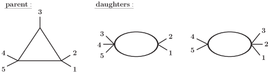
Figure 13: Parent and daughter integral functions. The Gram determinant singularity associated to the parent 3-point integral is $\Delta(K_{12},k_{3},K_{45})$. It is present in its integral coefficient as well as in the coefficients of both daughter 2-point integrals.

We thus obtain a recursion relation for the rational terms, which is exact near the Gram determinant singularities. Contour integrals whether continuous or discrete can then be used to extract the exact value of the spurious residues of eq. (105).

Thus obtained recursive approaches allow to compute rational terms from purely recursive methods, albeit, using a set of well chosen auxiliary shifts. These methods have already been applied for the computations of split helicity scattering amplitudes, needed in the computation of $W\,\!+3$-jet and $Z\,\!+3$-jet production [30, 32, 34] leading to greatly improved computation time for these pieces. A much wider class of computations seems in reach using the above newly developed recursive methods.

6 Conclusions

The computations of observable cross-sections rely on the composition of several components, which are linked through the fundamental QCD Lagrangian. Here we described modern approaches for evaluating the hard scattering part at next-to-leading order, which can be programmed. The value of a first principle understanding of scattering processes in addition to the increased quantitative control motivates the quest for cross sections at NLO.

The description of processes with complex final states at NLO is one of the central achievements of many recent developments of numerical on-shell [47, 19, 20, 21] and unitarity methods [22, 23, 25, 27, 21, 29]. These methods are already used by a new generation of tools [79, 21, 68, 133, 39, 40, 41, 38, 42]. Such numerical methods scale very well as the number of external states increases and have already lead to a new understanding for several proton scattering processes at hadron colliders [33, 35, 36, 37, 38] including $W/Z+3$-jet and $W+4$-jet production [30, 31, 32, 36]. Being key backgrounds to many new physics signals including supersymmetry searches, the explicit results emphasizes the importance of modern field-theory methods for precision prediction of hadron collider physics.

Numerical on-shell and unitarity methods allow us to automate computations of scattering amplitudes in a numerically stable and efficient way. These methods exploit, for example, the discontinuities across branch cuts to construct amplitudes. Efficiency and stability originates then in two facts: Firstly, discontinuities are expressed in terms of purely on-shell information, namely, on-shell tree-amplitudes. Evaluation of on-shell trees is fast and numerically stable. In addition, this allows us to ignore ghosts and gauge fixing altogether and reduces the use of redundant unphysical information.

These modern ideas presented here my also help with issues beyond the computation of matrix elements. New insights may impact on various other components of multi-jet computations. This includes subtraction methods for integrating parton level NLO computations, showering and formulation of new observables.

The central strategy, leading to the success and popularity of these developments, is to make maximal use of physical principles and mathematical structures in order to obtain efficient and robust phenomenology. This kind of work, is at the cross-roads of theory and phenomenology has led to many recent insights, on the more formal side [146, 147, 21, 29, 136, 148] as well as of more phenomenological nature [110].

References

References

- [1] G. P. Salam, arXiv:1011.5131 [hep-ph].
- [2] contribution of G. Dissertori and G. Salam, “Quantum Chromodynamics”, p.114 to KNakamura et al. [ Particle Data Group Collaboration ], J. Phys. G G37, 075021 (2010).
- [3] R. K. Ellis, W. J. Stirling and B.R. Webber, QCD and Collider Physics (Cambridge University Press, 1996).
- [4] M. L. Mangano, T. J. Stelzer, Ann. Rev. Nucl. Part. Sci. 55, 555-588 (2005).
- [5] L. J. Dixon, [arXiv:0712.3064 [hep-ph]].
- [6] T. Stelzer and W. F. Long, Comput. Phys. Commun. 81, 357 (1994) [hep-ph/9401258]; J. Alwall, P. Demin, S. de Visscher, R. Frederix, M. Herquet, F. Maltoni, T. Plehn, D. L. Rainwater et al., JHEP 0709, 028 (2007) [arXiv:0706.2334 [hep-ph]]; A. Pukhov et al., hep-ph/9908288; M. L. Mangano, M. Moretti, F. Piccinini, R. Pittau and A. D. Polosa, JHEP 0307, 001 (2003) [hep-ph/0206293].
- [7] A. Kanaki and C. G. Papadopoulos, Comput. Phys. Commun. 132, 306 (2000) [hep-ph/0002082]; A. Cafarella, C. G. Papadopoulos, M. Worek, Comput. Phys. Commun. 180 (2009) 1941-1955. [arXiv:0710.2427 [hep-ph]].
- [8] F. Krauss, R. Kuhn and G. Soff, JHEP 0202, 044 (2002) [hep-ph/0109036].
- [9] T. Gleisberg, S. Hoeche, JHEP 0812, 039 (2008). [arXiv:0808.3674 [hep-ph]].
- [10] M. Moretti, T. Ohl, J. Reuter, In *2nd ECFA/DESY Study 1998-2001* 1981-2009. [hep-ph/0102195]; W. Kilian, T. Ohl, J. Reuter, [arXiv:0708.4233 [hep-ph]].
- [11] H. U. Bengtsson and T. Sjöstrand, Comput. Phys. Commun. 46, 43 (1987); T. Sjöstrand, P. Eden, C. Friberg, L. Lönnblad, G. Miu, S. Mrenna and E. Norrbin, Comput. Phys. Commun. 135, 238 (2001) [hep-ph/0010017]; G. Marchesini and B. R. Webber, Cavendish-HEP-87/9, Dec 1987; G. Marchesini, B. R. Webber, G. Abbiendi, I. G. Knowles, M. H. Seymour and L. Stanco, Comput. Phys. Commun. 67, 465 (1992); G. Corcella et al., hep-ph/0210213.
- [12] T. Gleisberg, S. Höche, F. Krauss, M. Schönherr, S. Schumann, F. Siegert and J. Winter, JHEP 0902, 007 (2009) [0811.4622 [hep-ph]].
- [13] S. Catani, F. Krauss, R. Kuhn and B. R. Webber, JHEP 0111, 063 (2001) [hep-ph/0109231]; M. Mangano, presented at the Fermilab ME/MC Tuning Workshop, October 4, 2004.
- [14] M. L. Mangano, M. Moretti, F. Piccinini and M. Treccani, JHEP 0701, 013 (2007) [hep-ph/0611129]; S. Mrenna and P. Richardson, JHEP 0405, 040 (2004) [hep-ph/0312274].
- [15] Z. Bern et al., 0803.0494 [hep-ph].
- [16] S. Frixione and B.R. Webber, JHEP 0206, 029 (2002) [hep-ph/0204244]; S. Frixione, P. Nason and B.R. Webber, JHEP 0308, 007 (2003) [hep-ph/0305252]; S. Frixione, P. Nason and C. Oleari, JHEP 0711, 070 (2007) [0709.2092 [hep-ph]]; S. Alioli, P. Nason, C. Oleari and E. Re, JHEP 0807, 060 (2008) [0805.4802 [hep-ph]].
- [17] R. V. Harlander and W. B. Kilgore, Phys. Rev. Lett. 88, 201801 (2002) [hep-ph/0201206]; C. Anastasiou and K. Melnikov, Nucl. Phys. B 646, 220 (2002) [hep-ph/0207004]; C. Anastasiou, K. Melnikov and F. Petriello, Phys. Rev. Lett. 93, 262002 (2004) [hep-ph/0409088]; C. Anastasiou, K. Melnikov and F. Petriello, Nucl. Phys. B 724, 197 (2005) [hep-ph/0501130]; G. Davatz et al., JHEP 0607, 037 (2006) [hep-ph/0604077]; C. Anastasiou, G. Dissertori, F. Stöckli and B. R. Webber, JHEP 0803, 017 (2008) [0801.2682 [hep-ph]].
- [18] C. Anastasiou, L. J. Dixon, K. Melnikov and F. Petriello, Phys. Rev. D 69, 094008 (2004) [hep-ph/0312266]; K. Melnikov and F. Petriello, Phys. Rev. Lett. 96, 231803 (2006) [hep-ph/0603182]; K. Melnikov and F. Petriello, Phys. Rev. D 74, 114017 (2006) [hep-ph/0609070]; S. Frixione and M. L. Mangano, JHEP 0405, 056 (2004) [hep-ph/0405130]; N. E. Adam, V. Halyo, S. A. Yost, JHEP 0805 (2008) 062. [arXiv:0802.3251 [hep-ph]].
- [19] Z. Bern, L. J. Dixon and D. A. Kosower, Phys. Rev. D 71, 105013 (2005) [hep-th/0501240]; Phys. Rev. D 72, 125003 (2005) [hep-ph/0505055]; Phys. Rev. D 73, 065013 (2006) [hep-ph/0507005];
- [20] Z. Bern, N. E. J. Bjerrum-Bohr, D. C. Dunbar and H. Ita, JHEP 0511, 027 (2005) [arXiv:hep-ph/0507019].
- [21] C. F. Berger, Z. Bern, L. J. Dixon, F. Febres Cordero, D. Forde, H. Ita, D. A. Kosower and D. Maître, Phys. Rev. D 78, 036003 (2008) [0803.4180 [hep-ph]].
- [22] Z. Bern, L. J. Dixon, D. C. Dunbar and D. A. Kosower, Nucl. Phys. B 425, 217 (1994) [hep-ph/9403226]; Nucl. Phys. B 435, 59 (1995) [hep-ph/9409265].
- [23] Z. Bern and A. G. Morgan, Nucl. Phys. B 467, 479 (1996) [hep-ph/9511336]; Z. Bern, L. J. Dixon, D. C. Dunbar and D. A. Kosower, Phys. Lett. B 394, 105 (1997) [hep-th/9611127].
- [24] Z. Bern, L. J. Dixon and D. A. Kosower, Nucl. Phys. B 513, 3 (1998) [hep-ph/9708239].
- [25] R. Britto, F. Cachazo and B. Feng, Nucl. Phys. B 725, 275 (2005) [hep-th/0412103].
- [26] D. Forde, Phys. Rev. D75, 125019 (2007). [arXiv:0704.1835 [hep-ph]].
- [27] G. Ossola, C. G. Papadopoulos and R. Pittau, Nucl. Phys. B 763, 147 (2007) [hep-ph/0609007]; F. del Aguila, R. Pittau, JHEP 0407, 017 (2004). [hep-ph/0404120].
- [28] R. K. Ellis, W. T. Giele and Z. Kunszt, JHEP 0803, 003 (2008) [0708.2398 [hep-ph]].
- [29] W. T. Giele, Z. Kunszt and K. Melnikov, JHEP 0804, 049 (2008) [0801.2237 [hep-ph]].
- [30] C. F. Berger et al., Phys. Rev. Lett. 102, 222001 (2009) [0902.2760 [hep-ph]].
- [31] R. K. Ellis, K. Melnikov and G. Zanderighi, Phys. Rev. D 80, 094002 (2009) [0906.1445 [hep-ph]].
- [32] C. F. Berger et al., Phys. Rev. D 80, 074036 (2009) [0907.1984 [hep-ph]].
- [33] K. Melnikov, M. Schulze, JHEP 0908, 049 (2009). [arXiv:0907.3090 [hep-ph]]; K. Melnikov, M. Schulze, Nucl. Phys. B840, 129-159 (2010). [arXiv:1004.3284 [hep-ph]]; K. Melnikov, M. Schulze, A. Scharf, Phys. Rev. D83, 074013 (2011). [arXiv:1102.1967 [hep-ph]].
- [34] C. F. Berger et al., Phys. Rev. D 82, 074002 (2010) [1004.1659 [hep-ph]].
- [35] G. Bevilacqua, M. Czakon, C. G. Papadopoulos, R. Pittau and M. Worek, JHEP 0909, 109 (2009) [0907.4723 [hep-ph]]; G. Bevilacqua, M. Czakon, C. G. Papadopoulos and M. Worek, Phys. Rev. Lett. 104, 162002 (2010) [1002.4009 [hep-ph]]; G. Bevilacqua, M. Czakon, A. van Hameren, C. G. Papadopoulos, M. Worek, JHEP 1102, 083 (2011). [arXiv:1012.4230 [hep-ph]].
- [36] C. F. Berger, Z. Bern, L. J. Dixon, F. F. Cordero, D. Forde, T. Gleisberg, H. Ita, D. A. Kosower and D. Maître, Phys. Rev. Lett. 106, 092001 (2011) [arXiv:1009.2338 [hep-ph]].
- [37] T. Binoth, N. Greiner, A. Guffanti, J. P. Guillet, T. Reiter and J. Reuter, Phys. Lett. B 685, 293 (2010) [0910.4379 [hep-ph]]; T. Melia, K. Melnikov, R. Rontsch and G. Zanderighi, JHEP 1012, 053 (2010) [1007.5313 [hep-ph]].
- [38] V. Hirschi, R. Frederix, S. Frixione, M. V. Garzelli, F. Maltoni, R. Pittau, JHEP 1105, 044 (2011) [arXiv:1103.0621 [hep-ph]].
- [39] A. Lazopoulos, 0812.2998 [hep-ph];
- [40] J. C. Winter and W. T. Giele, 0902.0094 [hep-ph]; W. Giele, Z. Kunszt, J. Winter, Nucl. Phys. B840, 214-270 (2010). [arXiv:0911.1962 [hep-ph]].
- [41] P. Mastrolia, G. Ossola, T. Reiter, F. Tramontano, JHEP 1008, 080 (2010). [arXiv:1006.0710 [hep-ph]].
- [42] S. Badger, B. Biedermann, P. Uwer, [arXiv:1011.2900 [hep-ph]].
- [43] R. Britto, to appear in “Scattering Amplitudes in Gauge Theories”, special issue of Journal of Physics A, R. Roiban(ed), M. Spradlin(ed), A. Volovich(ed), “Loop amplitudes in gauge theories: modern analytic approaches,” [arXiv:1012.4493 [hep-th]].
- [44] F. A. Berends and W. T. Giele, Nucl. Phys. B 306, 759 (1988).
- [45] F. Caravaglios, M. Moretti, Phys. Lett. B358, 332-338 (1995).
- [46] P. Draggiotis, R. H. P. Kleiss, C. G. Papadopoulos, Phys. Lett. B439, 157-164 (1998) [hep-ph/9807207].
- [47] R. Britto, F. Cachazo and B. Feng, Nucl. Phys. B 715, 499 (2005) [hep-th/0412308]; R. Britto, F. Cachazo, B. Feng and E. Witten, Phys. Rev. Lett. 94, 181602 (2005) [hep-th/0501052].
- [48] F. Cachazo, P. Svrcek, E. Witten, JHEP 0409, 006 (2004). [hep-th/0403047].
- [49] L. J. Dixon, J. M. Henn, J. Plefka, T. Schuster, JHEP 1101, 035 (2011). [arXiv:1010.3991 [hep-ph]].
-
[50]
S. J. Parke, T. R. Taylor,
Phys. Lett. B157, 81 (1985);
Z. Kunszt, Nucl. Phys. B271, 333 (1986). - [51] J. M. Drummond, J. Henn, G. P. Korchemsky, E. Sokatchev, Nucl. Phys. B828, 317-374 (2010) [arXiv:0807.1095 [hep-th]]; A. Brandhuber, P. Heslop, G. Travaglini, Phys. Rev. D78, 125005 (2008) [arXiv:0807.4097 [hep-th]]; J. M. Drummond, J. M. Henn, J. Plefka, JHEP 0905, 046 (2009) [arXiv:0902.2987 [hep-th]]; J. M. Drummond, Class. Quant. Grav. 27, 214001 (2010) [arXiv:1010.2418 [hep-th]].
- [52] L. J. Mason, D. Skinner, JHEP 1001 (2010) 064. [arXiv:0903.2083 [hep-th]]. Hodges A, arXiv:0905.1473 [hep-th]; N. Arkani-Hamed, F. Cachazo, C. Cheung, J. Kaplan, JHEP 1003 (2010) 020. [arXiv:0907.5418 [hep-th]]. N. Arkani-Hamed, F. Cachazo, C. Cheung, JHEPA,1003,036. 2010 1003 (2010) 036. [arXiv:0909.0483 [hep-th]]. Mason L, Skinner D, JHEP 0911:045 (2009) [arXiv:0909.0250 [hep-th]]; M. Bullimore, L. J. Mason, D. Skinner, JHEP 1003 (2010) 070. [arXiv:0912.0539 [hep-th]]. J. Kaplan, JHEP 1003 (2010) 025. [arXiv:0912.0957 [hep-th]]. N. Arkani-Hamed, J. Bourjaily, F. Cachazo, J. Trnka, JHEP 1101 (2011) 108. [arXiv:0912.3249 [hep-th]].
- [53] A. Brandhuber, B. Spence and G. Travaglini, to appear in “Scattering Amplitudes in Gauge Theories”, special issue of Journal of Physics A, R. Roiban(ed), M. Spradlin(ed), A. Volovich(ed), “Tree-Level Formalism,” 1103.3477 [hep-th].
- [54] T. Gleisberg, F. Krauss, Eur. Phys. J. C53, 501-523 (2008). [arXiv:0709.2881 [hep-ph]].
- [55] M. H. Seymour, C. Tevlin, [arXiv:0803.2231 [hep-ph]]; R. Frederix, T. Gehrmann, N. Greiner, JHEP 0809, 122 (2008). [arXiv:0808.2128 [hep-ph]]; M. Czakon, C. G. Papadopoulos, M. Worek, JHEP 0908, 085 (2009). [arXiv:0905.0883 [hep-ph]]; K. Hasegawa, S. Moch, P. Uwer, Comput. Phys. Commun. 181, 1802-1817 (2010). [arXiv:0911.4371 [hep-ph]];
- [56] R. Frederix, S. Frixione, F. Maltoni, T. Stelzer, JHEP 0910, 003 (2009). [arXiv:0908.4272 [hep-ph]].
- [57] S. Frixione, Z. Kunszt, A. Signer, Nucl. Phys. B467, 399-442 (1996) [hep-ph/9512328]; S. Frixione, Nucl. Phys. B507, 295-314 (1997) [hep-ph/9706545].
- [58] S. Catani and M. H. Seymour, Phys. Lett. B 378, 287 (1996) [hep-ph/9602277]; Nucl. Phys. B 485, 291 (1997) [Erratum-ibid. B 510, 503 (1998)] [hep-ph/9605323].
- [59] D. A. Kosower, Phys. Rev. D57, 5410-5416 (1998). [hep-ph/9710213]; J. M. Campbell, M. A. Cullen, E. W. N. Glover, Eur. Phys. J. C9, 245-265 (1999) [hep-ph/9809429]; D. A. Kosower, Phys. Rev. D71, 045016 (2005) [hep-ph/0311272].
- [60] R. K. Ellis, W. T. Giele, G. Zanderighi, JHEP 0605, 027 (2006) [hep-ph/0602185]; R. K. Ellis, W. T. Giele, G. Zanderighi, Phys. Rev. D73, 014027 (2006) [hep-ph/0508308].
- [61] A. Bredenstein, A. Denner, S. Dittmaier and S. Pozzorini, JHEP 0808, 108 (2008) [0807.1248 [hep-ph]]; Phys. Rev. Lett. 103, 012002 (2009) [0905.0110 [hep-ph]].
- [62] S. Dittmaier, P. Uwer, S. Weinzierl, Phys. Rev. Lett. 98, 262002 (2007) [hep-ph/0703120 [HEP-PH]]; G. Belanger, F. Boudjema, J. Fujimoto, T. Ishikawa, T. Kaneko, K. Kato, Y. Shimizu, Phys. Rept. 430, 117-209 (2006) [hep-ph/0308080].
- [63] A. Denner and S. Dittmaier, Nucl. Phys. B 734, 62 (2006) [hep-ph/0509141].
- [64] W. T. Giele and E. W. N. Glover, JHEP 0404, 029 (2004) [hep-ph/0402152]; T. Binoth, J. P. Guillet, G. Heinrich, E. Pilon and C. Schubert, JHEP 0510, 015 (2005) [hep-ph/0504267]; A. Denner and S. Dittmaier, Nucl. Phys. B 734, 62 (2006) [hep-ph/0509141]. T. Binoth, J. -P. .Guillet, G. Heinrich, E. Pilon, T. Reiter, Comput. Phys. Commun. 180 (2009) 2317-2330 [arXiv:0810.0992 [hep-ph]].
- [65] A. Denner, S. Dittmaier, M. Roth and L. H. Wieders, Phys. Lett. B 612, 223 (2005) [hep-ph/0502063]; Nucl. Phys. B 724, 247 (2005) [hep-ph/0505042].
- [66] J. R. Andersen et al. [ SM and NLO Multileg Working Group Collaboration ], [arXiv:1003.1241 [hep-ph]].
- [67] D. Forde and D. A. Kosower, Phys. Rev. D 73, 061701 (2006) [hep-ph/0509358]; C. F. Berger, Z. Bern, L. J. Dixon, D. Forde and D. A. Kosower, Phys. Rev. D 75, 016006 (2007) [hep-ph/0607014]. C. F. Berger, Z. Bern, L. J. Dixon, D. Forde and D. A. Kosower, Phys. Rev. D 74, 036009 (2006) [hep-ph/0604195].
- [68] W. T. Giele and G. Zanderighi, JHEP 0806, 038 (2008) [0805.2152 [hep-ph]].
- [69] K. Melnikov and G. Zanderighi, Phys. Rev. D 81, 074025 (2010) [0910.3671 [hep-ph]].
- [70] A. van Hameren, C. G. Papadopoulos, R. Pittau, JHEP 0909 (2009) 106 [arXiv:0903.4665 [hep-ph]].
- [71] J. J. M. Carrasco, H. Johansson, to appear in “Scattering Amplitudes in Gauge Theories”, special issue of Journal of Physics A, R. Roiban(ed), M. Spradlin(ed), A. Volovich(ed), “Generic multiloop methods and application to N=4 super-Yang-Mills,” [arXiv:1103.3298 [hep-th]].
- [72] C. Anastasiou, R. Britto, B. Feng, Z. Kunszt and P. Mastrolia, Phys. Lett. B 645, 213 (2007) [hep-ph/0609191]; R. Britto and B. Feng, JHEP 0802, 095 (2008) [0711.4284 [hep-ph]].
- [73] F. A. Berends, R. Kleiss, P. De Causmaecker, R. Gastmans and T. T. Wu, Phys. Lett. B 103, 124 (1981); P. De Causmaecker, R. Gastmans, W. Troost and T. T. Wu, Nucl. Phys. B 206, 53 (1982); Z. Xu, D. H. Zhang and L. Chang, TUTP-84/3-TSINGHUA; J. F. Gunion and Z. Kunszt, Phys. Lett. B 161, 333 (1985); Z. Xu, D. H. Zhang and L. Chang, Nucl. Phys. B 291, 392 (1987).
- [74] M. L. Mangano and S. J. Parke, Phys. Rept. 200, 301 (1991); L. J. Dixon, in QCD & Beyond: Proceedings of TASI ’95, ed. D. E. Soper (World Scientific, 1996) [hep-ph/9601359].
- [75] F. A. Berends, W. Giele, Nucl. Phys. B294 (1987) 700.
- [76] Z. Bern and D. A. Kosower, Nucl. Phys. B 362, 389 (1991).
- [77] Z. Bern, L. J. Dixon, D. C. Dunbar and D. A. Kosower, Nucl. Phys. B 425, 217 (1994) [arXiv:hep-ph/9403226].
- [78] Z. Bern, L. J. Dixon and D. A. Kosower, Nucl. Phys. B 437, 259 (1995) [hep-ph/9409393].
- [79] G. Ossola, C. G. Papadopoulos and R. Pittau, JHEP 0803, 042 (2008) [0711.3596 [hep-ph]].
- [80] H. Fritzsch and P. Minkowski, Phys. Lett. B 73, 80 (1978); G. Altarelli, G. Parisi and R. Petronzio, Phys. Lett. B 76, 351 (1978); K. Kajantie and R. Raitio, Nucl. Phys. B 139, 72 (1978); K. Kajantie, J. Lindfors and R. Raitio, Nucl. Phys. B 144, 422 (1978).
- [81] R. Kleiss and W. J. Stirling, Nucl. Phys. B 262, 235 (1985).
- [82] S. D. Ellis, R. Kleiss and W. J. Stirling, Phys. Lett. B 154, 435 (1985).
- [83] M. L. Mangano and S. J. Parke, Phys. Rev. D 41, 59 (1990).
- [84] R. K. Ellis, G. Martinelli and R. Petronzio, Nucl. Phys. B 211, 106 (1983); W. T. Giele, E. W. N. Glover and D. A. Kosower, Nucl. Phys. B 403, 633 (1993) [hep-ph/9302225].
- [85] P. B. Arnold and M. H. Reno, Nucl. Phys. B 319, 37 (1989) [Erratum-ibid. B 330, 284 (1990)].
- [86] F. A. Berends, H. Kuijf, B. Tausk and W. T. Giele, Nucl. Phys. B 357, 32 (1991).
- [87] J. M. Campbell, R. K. Ellis, Phys. Rev. D65, 113007 (2002) [hep-ph/0202176].
- [88] F. Abe et al. [CDF Collaboration], Phys. Rev. Lett. 74, 2626 (1995) [hep-ex/9503002]; S. Abachi et al. [D0 Collaboration], Phys. Rev. Lett. 74, 2632 (1995) [hep-ex/9503003].
-
[89]
E. W. N. Glover and D. J. Miller,
Phys. Lett. B 396, 257 (1997)
[hep-ph/9609474];
Z. Bern, L. J. Dixon, D. A. Kosower and S. Weinzierl, Nucl. Phys. B 489, 3 (1997) [hep-ph/9610370];
J. M. Campbell, E. W. N. Glover and D. J. Miller, Phys. Lett. B 409, 503 (1997) [hep-ph/9706297]. - [90] J. M. Campbell and R. K. Ellis, Phys. Rev. D 65, 113007 (2002) [hep-ph/0202176].
- [91] W. T. Giele, S. Keller and E. Laenen, Phys. Lett. B 372, 141 (1996) [hep-ph/9511449].
- [92] J. M. Campbell, R. K. Ellis, F. Maltoni and S. Willenbrock, Phys. Rev. D 75, 054015 (2007) [hep-ph/0611348].
- [93] F. Febres Cordero, L. Reina, D. Wackeroth, Phys. Rev. D74, 034007 (2006) [hep-ph/0606102]; Phys. Rev. D78 (2008) 074014 [arXiv:0806.0808 [hep-ph]].
- [94] F. Febres Cordero, L. Reina and D. Wackeroth, Phys. Rev. D 74, 034007 (2006) [hep-ph/0606102]; F. Febres Cordero, L. Reina and D. Wackeroth, Phys. Rev. D 80, 034015 (2009) [0906.1923 [hep-ph]].
- [95] J. M. Campbell, R. K. Ellis, F. Febres Cordero, F. Maltoni, L. Reina, D. Wackeroth and S. Willenbrock, Phys. Rev. D 79, 034023 (2009) [0809.3003 [hep-ph]].
- [96] S. Badger, J. M. Campbell, R. K. Ellis, JHEP 1103, 027 (2011). [arXiv:1011.6647 [hep-ph]].
- [97] A. Bredenstein, A. Denner, S. Dittmaier and S. Pozzorini, JHEP 0808, 108 (2008) [0807.1248 [hep-ph]]; Phys. Rev. Lett. 103, 012002 (2009) [0905.0110 [hep-ph]]; JHEP 1003, 021 (2010) [1001.4006 [hep-ph]];
- [98] R. Frederix, S. Frixione, K. Melnikov, G. Zanderighi, JHEP 1011 (2010) 050 [arXiv:1008.5313 [hep-ph]].
- [99] M. L. Mangano, Eur. Phys. J. C59, 373-387 (2009). [arXiv:0809.1567 [hep-ph]]; J. A. Conley, J. S. Gainer, J. L. Hewett, M. P. Le, T. G. Rizzo, [arXiv:1103.1697 [hep-ph]].
- [100] G. Aad et al. [ The ATLAS Collaboration ], [arXiv:0901.0512 [hep-ex]].
- [101] G. L. Bayatian et al. [ CMS Collaboration ], J. Phys. G G34, 995-1579 (2007).
- [102] S. D. Ellis, R. Kleiss, W. J. Stirling, Phys. Lett. B154, 435 (1985); F. A. Berends, W. T. Giele, H. Kuijf, R. Kleiss, W. J. Stirling, Phys. Lett. B224, 237 (1989); F. A. Berends, H. Kuijf, B. Tausk, W. T. Giele, Nucl. Phys. B357, 32-64 (1991); E. Abouzaid, H. J. Frisch, Phys. Rev. D68, 033014 (2003). [hep-ph/0303088].
- [103] T. Aaltonen et al. [CDF Collaboration], Phys. Rev. D 77, 011108 (2008) [0711.4044 [hep-ex]].
- [104] T. Aaltonen et al. [ CDF - Run II Collaboration ], Phys. Rev. Lett. 100, 102001 (2008). [arXiv:0711.3717 [hep-ex]]. [105]
- [105] V. M. Abazov et al. [ D0 Collaboration ], Phys. Lett. B678, 45-54 (2009). [arXiv:0903.1748 [hep-ex]].
- [106] G. Aad et al. [ ATLAS Collaboration ], [arXiv:1012.5382 [hep-ex]].
- [107] C. W. Bauer, B. O. Lange, [arXiv:0905.4739 [hep-ph]].
- [108] See http://mcfm.fnal.gov .
- [109] L. J. Dixon, J. M. Henn, J. Plefka, T. Schuster, JHEP 1101, 035 (2011). [arXiv:1010.3991 [hep-ph]]; J. M. Drummond, J. Henn, G. P. Korchemsky and E. Sokatchev, Nucl. Phys. B 828, 317 (2010) [0807.1095 [hep-th]]; 0808.0491 [hep-th].
- [110] Z. Bern, G. Diana, L. J. Dixon, F. F. Cordero, D. Forde, T. Gleisberg, S. Hoeche, H. Ita et al., [arXiv:1103.5445 [hep-ph]].
- [111] Z. Bern, L. J. Dixon and D. A. Kosower, Annals Phys. 322, 1587 (2007) [0704.2798 [hep-ph]].
- [112] J. F. Gunion, Z. Kunszt, Phys. Lett. B176, 163 (1986). D. de Florian, J. Zurita, JHEP 0611, 080 (2006). [hep-ph/0609099].
- [113] Z. Bern, L. J. Dixon and D. A. Kosower, Ann. Rev. Nucl. Part. Sci. 46, 109 (1996) [hep-ph/9602280].
- [114] L. M. Brown and R. P. Feynman, Phys. Rev. 85, 231 (1952); L.M. Brown, Nuovo Cim. 21, 3878 (1961); B. Petersson, J. Math. Phys. 6, 1955 (1965); G. Källén and J.S. Toll, J. Math. Phys. 6, 299 (1965); D. B. Melrose, Nuovo Cim. 40, 181 (1965); G. Passarino and M. J. G. Veltman, Nucl. Phys. B 160, 151 (1979); Z. Bern, L. J. Dixon and D. A. Kosower, Phys. Lett. B 302, 299 (1993) [Erratum-ibid. B 318, 649 (1993)] [hep-ph/9212308]; J. Fleischer, F. Jegerlehner and O. V. Tarasov, Nucl. Phys. B 566, 423 (2000) [hep-ph/9907327]; T. Binoth, J. P. Guillet and G. Heinrich, Nucl. Phys. B 572, 361 (2000) [hep-ph/9911342]; G. Duplanc̆ić and B. Niz̆ić, Eur. Phys. J. C 35, 105 (2004) [hep-ph/0303184].
- [115] W. L. van Neerven and J. A. M. Vermaseren, Phys. Lett. B 137, 241 (1984);
- [116] G. ’t Hooft and M. J. G. Veltman, Nucl. Phys. B 153, 365 (1979); G. J. van Oldenborgh and J. A. M. Vermaseren, Z. Phys. C 46, 425 (1990); W. Beenakker and A. Denner, Nucl. Phys. B 338, 349 (1990); A. Denner, U. Nierste and R. Scharf, Nucl. Phys. B 367, 637 (1991); Z. Bern, L. J. Dixon and D. A. Kosower, Nucl. Phys. B 412 (1994) 751 [hep-ph/9306240]; T. Hahn and M. Pérez-Victoria, Comput. Phys. Commun. 118, 153 (1999) [hep-ph/9807565]; R. K. Ellis and G. Zanderighi, JHEP 0802, 002 (2008) [0712.1851 [hep-ph]].
- [117] J. Gluza, K. Kajda, D. A. Kosower, Phys. Rev. D83, 045012 (2011). [arXiv:1009.0472 [hep-th]].
- [118] F. Cachazo, [arXiv:0803.1988 [hep-th]].
- [119] S. J. Parke, T. R. Taylor, Phys. Rev. Lett. 56, 2459 (1986).
- [120] V. P. Nair, Phys. Lett. B214, 215 (1988).
- [121] M. T. Grisaru, H. N. Pendleton and P. van Nieuwenhuizen, Phys. Rev. D 15, 996 (1977); M. T. Grisaru and H. N. Pendleton, Nucl. Phys. B 124, 81 (1977).
- [122] J. L. Bourjaily, [arXiv:1011.2447 [hep-ph]].
- [123] Z. Bern, L. J. Dixon and D. A. Kosower, Phys. Rev. Lett. 70, 2677 (1993) [hep-ph/9302280].
- [124] S. D. Badger, JHEP 0901, 049 (2009) [0806.4600 [hep-ph]]; S. D. Badger, Nucl. Phys. Proc. Suppl. 183, 220 (2008) [0807.1245 [hep-ph]].
- [125] Z. Bern, Y. -t. Huang, to appear in “Scattering Amplitudes in Gauge Theories”, special issue of Journal of Physics A, R. Roiban(ed), M. Spradlin(ed), A. Volovich(ed), “Basics of Generalized Unitarity,” [arXiv:1103.1869 [hep-th]].
- [126] R.J. Eden, P.V. Landshoff, D.I. Olive, J.C.Polkinghorne, The Analytic S-Matrix (Cambridge University Press, 1966); G.F. Chew, S-Matrix Theory of Strong Interactions, ed. D.Pines , (Frontiers in physics; A Lecture Note and Reprint Series; W.A. Benjamin, 1961)
- [127] R. E. Cutkosky, J. Math. Phys. 1, 429-433 (1960).
- [128] L. D. Landau, Nucl. Phys. 13, 181-192 (1959)
- [129] W. L. van Neerven, Nucl. Phys. B268, 453 (1986).
- [130] R. Britto, B. Feng and P. Mastrolia, Phys. Rev. D 78, 025031 (2008) [0803.1989 [hep-ph]];
- [131] G. Ossola, C. G. Papadopoulos and R. Pittau, JHEP 0805, 004 (2008) [[0802.1876 [hep-ph]].
- [132] R. K. Ellis, W. T. Giele, Z. Kunszt and K. Melnikov, Nucl. Phys. B822 (2009) 270-282 [arXiv:0806.3467 [hep-ph]].
- [133] R. K. Ellis, W. T. Giele, Z. Kunszt, K. Melnikov and G. Zanderighi, JHEP 0901, 012 (2009) [0810.2762 [hep-ph]].
- [134] G. Mahlon, Phys. Rev. D 49, 2197 (1994) [hep-ph/9311213]; G. Mahlon, Phys. Rev. D 49, 4438 (1994) [hep-ph/9312276].
- [135] D. C. Dunbar, J. H. Ettle, W. B. Perkins, JHEP 1006, 027 (2010) [arXiv:1003.3398 [hep-th]].
- [136] N. Arkani-Hamed, J. L. Bourjaily, F. Cachazo, S. Caron-Huot and J. Trnka, JHEP 1101, 041 (2011) [arXiv:1008.2958 [hep-th]].
- [137] Schwinn C, Weinzierl S, JHEP 0704:072 (2007) [arXiv:hep-ph/0703021]; Badger SD, Glover EWN, Khoze VV, Svrček P, JHEP 0507:025 (2005) [arXiv:hep-th/0504159]; Badger SD, Glover EWN, Khoze VV, JHEP 0601:066 (2006) [arXiv:hep-th/0507161].
- [138] Bedford J, Brandhuber A, Spence BJ, Travaglini G, Nucl. Phys. B 721:98 (2005) [arXiv:hep-th/0502146]; Cachazo F, Svrček P, arXiv:hep-th/0502160; Bjerrum-Bohr NEJ, et al., JHEP 0601:009 (2006) [arXiv:hep-th/0509016]; Benincasa P, Boucher-Veronneau C, Cachazo F, JHEP 0711:057 (2007) [arXiv:hep-th/0702032]; Brandhuber A, McNamara S, Spence B, Travaglini G, JHEP 0703:029 (2007) [arXiv:hep-th/0701187]; Elvang H, Freedman DZ, Kiermaier M, JHEP 0904:009 (2009) [arXiv:0808.1720 [hep-th]]; Elvang H, Freedman DZ, Kiermaier M, JHEP 0906:068 (2009) [arXiv:0811.3624 [hep-th]].
- [139] R. Britto, B. Feng, R. Roiban, M. Spradlin and A. Volovich, Phys. Rev. D 71:105017 (2005) [arXiv:hep-th/0503198]; D. Forde and D. A. Kosower, Phys. Rev. D 73:065007 (2006) [arXiv:hep-th/0507292]; Drummond JM, Henn JM, JHEP 0904:018 (2009) [arXiv:0808.2475 [hep-th]].
- [140] Z. Bern and G. Chalmers, Nucl. Phys. B 447, 465 (1995) [hep-ph/9503236].
- [141] R. Britto, B. Feng, P. Mastrolia, Phys. Rev. D73, 105004 (2006). [hep-ph/0602178].
- [142] Z. Bern, L. J. Dixon and D. A. Kosower, Phys. Rev. D 71, 105013 (2005) [hep-th/0501240]; Phys. Rev. D 72, 125003 (2005) [hep-ph/0505055].
- [143] C. F. Berger, Z. Bern, L. J. Dixon, D. Forde and D. A. Kosower, Phys. Rev. D 75, 016006 (2007) [arXiv:hep-ph/0607014].
- [144] Z. Bern, L. J. Dixon and D. A. Kosower, Phys. Lett. B 302, 299 (1993) [Erratum-ibid. B 318, 649 (1993)] [hep-ph/9212308].
- [145] C. F. Berger, D. Forde, Ann. Rev. Nucl. Part. Sci. 60 (2010) 181-205. [arXiv:0912.3534 [hep-ph]].
- [146] C. Anastasiou, Z. Bern, L. J. Dixon, D. A. Kosower, Phys. Rev. Lett. 91, 251602 (2003). [hep-th/0309040]; Z. Bern, L. J. Dixon, V. A. Smirnov, Phys. Rev. D72, 085001 (2005). [hep-th/0505205].
- [147] Z. Bern, J. J. Carrasco, L. J. Dixon, H. Johansson, D. A. Kosower and R. Roiban, Phys. Rev. Lett. 98, 161303 (2007) [arXiv:hep-th/0702112]; Z. Bern, J. J. M. Carrasco, L. J. Dixon, H. Johansson, R. Roiban, Phys. Rev. D78, 105019 (2008). [arXiv:0808.4112 [hep-th]]; Z. Bern, J. J. Carrasco, L. J. Dixon, H. Johansson and R. Roiban, Phys. Rev. Lett. 103, 081301 (2009) [arXiv:0905.2326 [hep-th]].
- [148] N. Arkani-Hamed, J. L. Bourjaily, F. Cachazo, J. Trnka, [arXiv:1012.6032 [hep-th]].