1 Introduction

Correlations among spikes, both on the same neuron and across neurons, are ubiquitous in the brain. For example cross-correlograms can have large peaks, at least in the periphery [Rodieck1967, Mastronarde1983a, Mastronarde1983b, Nirenberg et al.2001, Dan et al.1998], and smaller – but still non-negligible – ones in cortex (see Cohen11 for a review), and auto-correlograms almost always exhibit non-trivial temporal structure at a range of timescales [Kim et al.1990, Bair et al.2001, Deger et al.2011]. Although this has been known for over forty years, it’s still not clear what role these correlations play in the brain – and, indeed, whether they play any role at all. The goal of this chapter is to shed light on this issue.

If synchronous spikes, or other temporal structures, are to play a role in the brain, they must convey something of interest – either about the outside world or about some internal state. One example of this comes from the so-called “binding hypothesis” [Milner1974, von der Malsburg1981, Gray1999] in which the rate of synchronous spikes across two neurons tells us whether two objects should be bound together (Fig. 9.1a). Alternatively, arbitrary patterns of spikes, rather than just synchronous ones, could be used to signal information about the outside world [Staude et al.2010] (Fig. 9.1b). In both cases, the spike patterns act as an extra channel of information; information is also carried by overall firing rate.

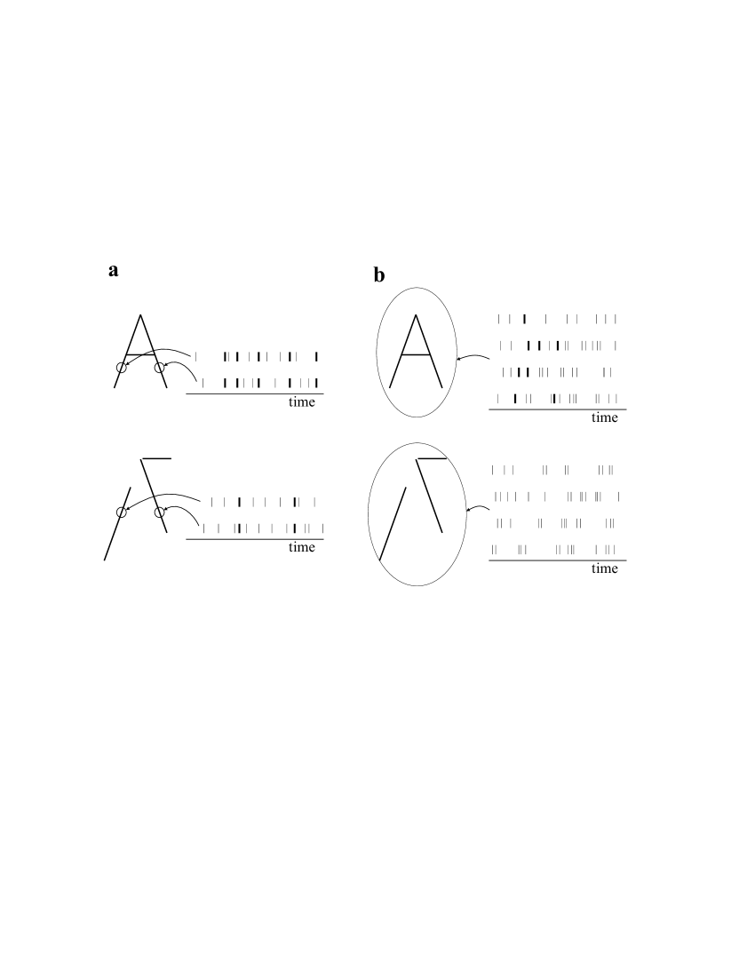
Figure 1: Illustrative examples of synchrony and spike pattern codes. a. Synchrony code. The circles in the top and bottom panels represent the receptive fields of two neurons; the vertical bars represent spike times. In the top panel, the neurons are activated by lines associated with a well known symbol, the letter A; to signal this, the neurons emit a large number of synchronous spikes (thick bars). In the bottom panel, the neurons are activated by a mainly random set of lines, and so the number of synchronous spikes (again shown as thick bars) is at chance. (in this case the position, orientation and length of the set of lines), and there is an additional spike pattern code for well known symbols. In the top panel, the image is, again, an A; the associated spike pattern code for the A is indicated by thick bars. In the bottom panel the lines are mainly random, and so there is no additional spike pattern code.

A key feature of these codes is that the degree of synchrony or the rate at which patterns occur is stimulus modulated, which automatically implies that the degree of correlations in the spike trains is stimulus modulated. For this reason, we refer to these as correlation-based neural codes. (Here when we refer to correlations we mean correlations conditioned on stimulus – so-called noise correlations, a point that is covered in detail in Chapter XI. In addition, we use the standard neuroscience convention, which is that correlations refer to correlations at all orders, not just covariance, as is common in the statistics literature.). To demonstrate that such correlation-based neural codes exist, then, one merely needs to look for stimulus-modulated correlations. This, however, is harder than it sounds, primarily because if synchronous spikes – or spike patterns – are an important component of the neural code (at least important from an information-theory perspective), they need to carry information not carried in firing rate. If, for instance, whenever the rate of synchronous spikes increases, so do firing rates, the brain could look at firing rate – which is, typically, far easier to estimate – and ignore synchronous spikes altogether. Of course, it would not have to do this; it could instead look at synchronous spikes, and ignore firing rate. However, demonstrating that experimentally is highly nontrivial. If, on the other hand, synchronous spikes carry extra information, then if the brain wants that information, it has to pay attention to correlations.

In this chapter we discuss quantitative methods for determining what role correlations play. By way of background, we start with a general discussion of the neural coding problem – which is to determine what aspects of spike trains carry information. Here we take the point of the brain, so “important” means “modify the brain’s view of what is going on in the outside world.” We then introduce a measure of the importance of correlations to the brain, and discuss what has been found using this measure, what it does (and doesn’t) mean, and how it can be estimated for large population. We end with a brief discussion of future directions.

2 The neural coding problem

The brain receives a steady stream of sensory information from the external world, a stream that is translated into spike trains by peripheral sensors (e.g., hair cells in the auditory system and photoreceptors in the retina). The job of the sensory system is to make sense of those spike trains; that is, use them to construct, either explicitly or implicitly, a representation of the outside world. In the neural coding field, we generally use $s$ to denote sensory stimuli (e.g. sounds or visual scenes) and ${\bf r}$ to denote neural activity. The transformation from sensory information to spike trains, is, then, a transformation from $s$ to ${\bf r}$, and the job of the brain is to invert that transformation, and construct a mapping from ${\bf r}$ to $s$.

An important feature of this transformation that it is stochastic: if one were to record from, say, retinal ganglion cells (the output cells of the retina) while showing exactly the same stimulus over and over, one would record a different pattern of spike trains each time the stimulus was shown. This probabilistic transformation is denoted $p({\bf r}|s)$, which we refer to as the conditional response distribution. It is not, though, the quantity of fundamental interest to the brain; what the brain really needs is $p(s|{\bf r})$, the probability distribution of stimuli given responses, known as the posterior distribution. That quantity is related to $p({\bf r}|s)$ via Bayes’ theorem,

$$p(s|{\bf r})=\frac{p({\bf r}|s)p(s)}{p({\bf r})}$$ (1)

where $p(s)$ is the prior distribution over stimuli and $p({\bf r})$ is the total response distribution, given by

$$p({\bf r})=\sum_{s}p({\bf r}|s)p(s)\,.$$ (2)

The denominator in Eq. (1), $p({\bf r})$, ensures that $p(s|{\bf r})$ is properly normalized, meaning $\sum_{s}p(s)=1$. (If the stimulus is continuous, sums over $s$ are replaced by integrals.)

An important feature of Eq. (1) is that the response, ${\bf r}$, carries information about the full distribution of stimuli, not just about one single stimulus. Thus, when we say that the problem faced by the sensory system is to make sense of incoming spike trains, what we mean is that the problem faced by the brain is to compute $p(s|{\bf r})$, or at least compute an approximation to it. Of course, there is no guarantee that the brain really does this. Instead, it could simply associate a single stimulus with each neural response. This is an important possibility to consider, because computing full probability distributions if far harder than estimating single values. However, it seems to be an unlikely possibility: even for something as simple as crossing the street when there is an oncoming car, it is necessary to estimate when the car will reach us and attach error bars to that estimate; without error bars it would be impossible to make a good decision. And, indeed, there is mounting evidence that the brain does take into account uncertainty when making decisions [Jacobs1999, Ernst and Banks2002, Körding and Wolpert2004, Chater et al.2006, Ma et al.2011]; uncertainty that can only come from $p(s|{\bf r})$. Here, then, we consider full posteriors.

So far this is all very straightforward. However, although Eq. (1) is highly compact, it is not easy to work with, for two reasons. First, the set of stimuli is infinite, and it has a structure that is very hard to capture mathematically. This makes it effectively impossible to determine the probability of every stimulus (imagine, for example, trying to determine the probability of every possible image). Consequently, the prior, $p(s)$, cannot be known, let alone written down. Second, the response, ${\bf r}$, consists of a set of spike times, and so lives in an infinite dimensional space. Thus, the same pattern of activity never occurs twice, making it impossible to estimate $p({\bf r}|s)$ from data if we stick to a pure spike time representation.

The first problem we ignore altogether (a common, although not universal, strategy in the neural coding field): rather than considering realistic stimuli, we consider a relatively small set of discrete stimuli, and simply assign a probability to each of them. For example, when investigating the visual system, we might show images consisting of a set of oriented bars at 12 different angles, and assign each of them a probability of 1/12.

This is a huge simplification, because it means if we know $p({\bf r}|s$), computing $p(s|{\bf r})$ via Bayes’ theorem is straightforward. Thus, we can focus solely on $p({\bf r}|s)$. However, it too is very high dimensional, so estimating it is still a hard problem. Importantly, the brain has the same hard problem: it, like us, has to learn what spike times mean – that is, learn how to translate from responses to stimuli, via Eq. (1). Since it never sees the same set of spike trains twice, it can’t use a pure spike time representation; if it did, every spike train would look new, and it would never learn anything.

The solution, of course, is to apply some sort of regularization, so that spike trains that are close mean approximately the same thing. Because the brain is a mechanistic device, this happens naturally (barring issues of chaotic dynamics, which is a topic in itself; see, for example, London2010). We as neuroscientists would like to know what regularization the brain uses. This is the neural coding problem, and it has dominated the neural coding field for the last several decades.

Importantly, what regularization the brain uses – that is, what neural code it uses – has consequences that go well beyond the neural coding field. Consider, for example, two possible neural codes. In one, different spike trains are considered close if there are about the same number of spikes on each neuron in any 100 ms interval (a spike count code); in the other, different spike trains are considered close if most of the spikes occur within about 1 ms of each other (a spike timing code).

Networks that compute with these two neural codes are highly likely to look very different. Therefore, before building computational models of the brain, we need to understand what the neural code is.

3 Approximate distributions and the neural code

It is, unfortunately, next to impossible to directly determine what kind of regularization the brain uses – that would almost require a complete theory of sensory processing. We can, however, determine this indirectly if we’re willing to make one assumption: if there is information in spike trains, the brain uses it. With that assumption, we can try out different regularizations and see which one provides the most information about the stimulus.

There are, basically, two ways to do this. The one that was popular in the 1980s and 90s [Optican and Richmond1987, Richmond and Optican1990, Bialek et al.1991, Bialek and Rieke1992], and continues to be used today [Ince et al.2010, Kayser et al.2010], is the direct approach, in which we choose a regularization; that is, we define explicitly what it means for two spike trains to be close. For example, we could discretize time into bins, and replace spike times by spike count on each neuron in each time bin. This is equivalent to defining ${\bf r}$ to be a set of spike counts rather than spike times, and it means that two spike trains are considered exactly the same if they have the same spike counts for all neurons in all bins, even if the spikes occurred at different times. Analysis then proceeds by computing the mutual information [Shannon and Weaver1949] between stimuli and responses versus bin size. (For a review of information theory, especially how it is used in neuroscience, see Chapter XI). Other notions of closeness that have been used are principal components [Optican and Richmond1987, Richmond and Optican1990, Eskandar et al.1992, Gawne and Richmond1993, Gawne et al.1996, Wiener and Richmond1999] and a metric that measures distance in terms of how much one has to move spikes and add or delete them to make two spike trains identical [Victor and Purpura1996, Victor2005]. Here, though, we consider only binned spike trains.

The other approach is to use an approximate distribution, which we denote $q({\bf r}|s)$, in place of $p({\bf r}|s)$. This approach, which was popular in the 1960s and 70s [Marmarelis and Marmarelis1978], fell out of favor when information theory was introduced, but has gained a resurgence of popularity in the last decade [Truccolo et al.2005]. Note that it includes the previous approach, for which $q({\bf r}|s)=p({\bf f}({\bf r})|s)$ where ${\bf f}({\bf r})$ is a mapping that respects the relevant notion of closeness (e.g., for binned spike trains, ${\bf f}({\bf r})$ maps spike times to spike counts). However, it gives us a much broader class of approximate distributions, and thus much more flexibility. It does, though, slightly change the neural coding problem: rather than asking, say, what bin size is relevant to the brain, it asks what approximate distribution takes us closest to the true posterior.

Which approach is better? The answer is not immediately obvious.. There are two advantages to using explicit regularizations. The first is that it is conceptually straightforward. The second is that it is easy to determine how much information is lost by any particular regularization. That’s because the mapping from ${\bf r}$ to ${\bf f}({\bf r})$ can at best preserve information, and usually leads to information loss. Thus, if we binned spikes, we could ask how much information is lost as a function of bin size. At some sufficiently small bin size we would find that almost no information is lost; the size of this bin is the timescale that matters in the brain (assuming that the brain really wants all available information).

There is, though, a downside to using an explicit regularization, or at least to binning spikes: it requires a large amount of data. One reason is that as the bin size get smaller, it becomes harder and harder to estimate the probability of a spike in any one bin: the number of trials required to accurately estimate that probability is inversely proportional to the bin size (which follows because for small enough bin size, spiking becomes Bernoulli). And if the probability can’t be estimated accurately, the information can’t be computed accurately. A related reason has to do with correlations: the number of spikes in one bin is correlated with the number of spikes in other bins. Thus, we really need the joint probability of spiking across bins. If, for example, we had $10$ bins, at small enough bins sizes that there could be at most one spike in each of them, there are 1024 ($2^{10}$) possible responses, and we need to compute the probability of each of them – a daunting task. The problem becomes exponentially harder as the number of neurons increases, because with each neuron we get 10 more bins. Even for only 10 neurons, there are 100 bins, and so about $10^{30}$ possible spike patterns – and, again, we need to compute the probability of each of them! This exponential increase is the curse of dimensionality, and it’s what makes population coding so hard.

For that reason, we are typically better off using an approximate distribution rather than directly regularizing spike trains. This gives us the freedom to choose a parametrization for which the number of parameters does not grow exponentially with the number of neurons. Instead, typically it can be chosen to grow linearly or quadratically, making it feasible to determine the approximate distribution from data. Of course, this approach also has a downside. When we bin spikes and compute the probability distribution over spike counts, we have only two sources of error: estimation error and error associated with the information we have thrown away by using finite bin sizes. When we use an approximate distribution, we are typically using the wrong distribution. This requires us to be careful about how we assess the quality of the approximate distribution we use. This is the subject of the next section.

4 Assessing the quality of approximate distributions: ${\Delta I}$

In practice, we often (although not always) use a mix of the two approaches described in the previous section: we bin spikes, and then, based on the resulting spike count code, we use an approximate distribution. For simplicity, here we discretize time into only one bin, so that ${\bf r}\rightarrow{\bf n}\equiv(n_{1},n_{2},...,n_{N})$ where $n_{i}$ is the spike count on neuron $i$ and there are $N$ neurons. (We could, of course, discretize time into multiple bins, but this would add nothing conceptually; the only effect would be to turn the $n_{i}$ into vectors of spike counts.) The approximation conditional response distribution is, then, given by $q({\bf n}|s)$ and, in a slight abuse of notation, we define the true distribution to be $p({\bf n}|s)$. Note that this is only a slight abuse: $p({\bf n}|s)$ is the true distribution of spike counts; it just doesn’t tell us the true distribution over spike times.

Associated with the approximate conditional response distribution, $q({\bf n}|s)$, is an approximate posterior; in analogy to Bayes’ theorem, Eq. (1), it is given by

$$q(s|{\bf n})=\frac{q({\bf n}|s)p(s)}{q({\bf n})}$$ (3)

where $q({\bf n})$ is the approximate total response distribution, $q({\bf n})=\sum_{s}q({\bf n}|s)p(s)$. Note that we are using the correct prior. It too could be approximated, but we do not discuss that here.

This leaves us with two questions: How do we determine how close $q({\bf n}|s)$ is to the true posterior distribution, $p({\bf n}|s)$? And what approximate conditional response distribution do we use? There is no one answer to the first question, as there are many ways to compare distributions, and the correct one should depend on the goal of the organism under study. One approach, proposed by Amari and colleagues, is based on the Fisher information available to an approximate decoder [Wu et al.2000, Wu et al.2001]. That measure, however, can not be used with discrete stimuli, so here we use a somewhat generalized version of their measure. It is based on what is probably the most natural measure of distance between probability distributions, the Kullback-Leibler distance, denoted $D_{KL}\big{(}p(s|{\bf n})||q(s|{\bf n})\big{)}$. This quantity (which is not a true distance [Kullback and Leibler1951]) is given by

$$D_{KL}\big{(}p(s|{\bf n})||q(s|{\bf n})\big{)}=\sum_{s}p(s|{\bf n})\log\frac{p(s|{\bf n})}{q(s|{\bf n})}\,.$$ (4)

This is the distance for a particular response; to get a response independent measure, we average over all responses weighted by their probability of occurring. The resulting quantity, denoted ${\Delta I}$, is given by [Nirenberg et al.2001, Nirenberg and Latham2003, Latham and Nirenberg2005]

$${\Delta I}=\sum_{\bf n}p({\bf n})D_{KL}\big{(}p(s|{\bf n})||q(s|{\bf n})\big{)}\,.$$ (5)

Note that because ${\Delta I}$ is based on the Kullback-Leibler distance, it is zero only if $q(s|{\bf n})=p(s|{\bf n})$ for all stimuli; if $q(s|{\bf n})\neq p(s|{\bf n})$ for even one stimulus, it is positive. Throughout most of this chapter we use ${\Delta I}$ as our measure of the quality of an approximate distribution. Below we discuss in more depth its meaning, its limitations, and, briefly, other possible measures.

The second question, “what approximate distribution do we use?”, doesn’t have an easy answer, in large part because there are essentially no restrictions on this distribution. To choose a sensible approximation, we need a better handle on what question we’re interested in. For that we take a close look at population coding.

5 Population coding

A potentially interesting, and potentially powerful, feature of population coding is the possibility of nontrivial structure in spike trains, as discussed in the introduction in the context of the the binding hypothesis and spike pattern codes (see in particular Fig. 9.1). If such nontrivial structure does exist, there are several far-reaching consequences. Probably the most important – and often overlooked – is that the brain must have the machinery to generate synchronous spikes or precise patterns of activity that carry information about the stimulus. Consequently, whether or not such structures exist is an extremely important question, since it affects, in a very fundamental way, how we think about how the brain carries out computations.

A second, also important, consequence is that if there really is nontrivial structure in the spike trains, it means that neurons act together to represent the world. Uncovering that representation requires, at the very least, paired recordings – and in the case of spike pattern codes, simultaneous recordings from a potentially large number of neurons. Thus, computational issues aside, from a purely pragmatic point of view it is important to know whether they exist.

The fact that nontrivial structure (or at least nontrivial structure as we have defined it here) can be seen only when neurons are recorded simultaneously suggests a natural approximate distribution: one in which simultaneously recorded neurons are replaced with neurons recorded on separate trials. This is equivalent to assuming independence, for which the approximate conditional response distribution, which we denote $q_{ind}({\bf n}|s)$, is given by

$$q_{ind}({\bf n}|s)=\prod_{i}p(n_{i}|s)$$ (6)

where $p(n_{i}|s)$ is the single neuron conditional response distribution. Here the parametrization is the single neuron conditional response distribution under a spike count assumption. This has a very convenient feature: it removes the curse of dimensionality. That’s because if there are $k$ possible responses for each neuron ($n_{i}$ can take on $k$ different values) and $N$ neurons, then for each stimulus, $s$, we need only $N(k-1)$ numbers to fully characterize $q_{ind}({\bf n}|s)$ (we need $N(k-1)$ numbers rather than $Nk$ because $p(n_{i}|s)$ is a normalized probability distribution). For even moderate $N$, this is many orders of magnitude smaller than the $k^{N}$ numbers (more accurately, $k^{N}-1$, again because of the normalization) we typically need to characterize the full distribution, $p({\bf n}|s)$.

By using the independent distribution as the approximate one, it seems that we are getting to the heart of the question “are correlations important?”. Indeed, suppose $q_{ind}(s|{\bf n})=p(s|{\bf n})$ for all stimuli (recall that $q_{ind}(s|{\bf n})$ is given by Eq. (3)). In that case, downstream areas in the brain could both decode responses perfectly and perform computations optimally without knowing anything about correlations. In the opposite case, $q_{ind}(s|{\bf n})\neq p(s|{\bf n})$ for at least one stimulus, the brain would have to know about correlations. We are tempted, then, to make the statement “correlations are unimportant if $q_{ind}(s|{\bf n})=p(s|{\bf n})$, and important otherwise.” Alternatively, because ${\Delta I}$ is zero if and only if $q_{ind}(s|{\bf n})=p(s|{\bf n})$ for all stimuli (see Eq. (5)), this statement is equivalent to “correlations are unimportant if and only if ${\Delta I}=0$.”

Indeed, from a purely information theory and optimal computing point of view, this is correct. However, from the point of view of the brain, the situation is more nuanced. In Sec. 10 we expand on this point. First, though, we need a better understanding of some of the mathematical properties of ${\Delta I}$, and we also need to consider alternative approaches. In the next several sections, then, we provide an information-theoretic interpretation of ${\Delta I}$, provide examples in which the responses are highly correlated and ${\Delta I}=0$, take a look at the experimental data on ${\Delta I}$, consider two alternative approximate distributions, and look at another measure of the role of correlations.

6 An information-theoretic perspective on ${\Delta I}$

If we did an experiment and found that ${\Delta I}=0$, the result would be easy to interpret: the posterior distribution over stimuli computed from the independent conditional distribution is exactly the same as that computed from the true conditional distribution. However, experimentally we almost never find that ${\Delta I}=0$; besides the fact that correlations almost always play some role, even if ${\Delta I}$ really were zero, when computed from finite data it typically becomes positive. So how do we interpret positive values of ${\Delta I}$? Our favorite interpretation is that it is the penalty one pays, in yes/no question, in guessing the stimulus (an interpretation that is independent of whether or not $q({\bf n}|s)$ is the independent distribution, $q_{ind}({\bf n}|s)$, or some other one). This interpretation is discussed in some detail in Nirenberg03; here we review it briefly.

Suppose that rather than computing the posterior distribution over stimuli, we guessed the stimuli using yes/no questions. An example of an allowed question, in the case of four stimuli, is “is it stimulus 1, 3 or 4?”. Once that question is answered, we get to ask another one, and the process continues until we know exactly what the stimulus is. The optimal question asking strategy is to divide the total probability of the stimulus in half with each question. This is a generalization of the approach to answering the question “We’re thinking of a number between 1 and 1024; what is it?”. Assuming a uniform prior, the first question would be something like “is it between 1 and 512?”, and each subsequent questions would reduce the number of possibilities by a factor of two. For a non-uniform prior, however, the strategy is different. If, for instance, you knew that we always chose a number between 1 and 512, the first question would be something like “is it between 1 and 128?”.

While this seems like a rather artificial approach to neural coding, it turns out that it can be directly related to mutual information. In fact, the difference in the average number of yes/no questions it takes to guess the stimulus before and after receiving a response is the mutual information (a statement that is largely correct, but requires some caveats associated with batch coding [Cover and Thomas1991]). To guess the stimulus in the minimum number of questions, one has to know the true posterior; if an approximate posterior is used, it will take more questions. This was obvious in the previous example: if the question-asker had not known that we always choose a number between 1 and 512, she would have taken one extra question. That this is true in general is slightly less obvious, but is not hard to show; see, for example, [Cover and Thomas1991]. It also suggests a natural metric against which ${\Delta I}$ should be measured: the true mutual information, denoted $I$, which is the reduction in yes/no questions one gets by observing the stimulus [Cover and Thomas1991, Nirenberg and Latham2003].

Note that while ${\Delta I}$ is a yes/no question cost, and yes/no questions look a lot like bits, it’s not a true information loss. In fact, ${\Delta I}$ can exceed the information [Schneidman et al.2003a], something that happens when the approximate distribution is, on average, worse than the prior distribution (at least as measured by yes/no questions). However, as shown in [Latham and Nirenberg2005], it is an upper bound on information loss. Consequently, small values of ${\Delta I}$ are meaningful.

Although ${\Delta I}$ has a relatively intuitive interpretation, is it really necessary to bother with this quantity? Why not simply ask how correlated responses are? The answer is that just because correlations exist doesn’t mean they are important for determining the posterior distribution over stimuli. In other words, the question “is $q(s|{\bf n})$ close to $p(s|{\bf n})$?” – which we are asking here, and which ${\Delta I}$ answers – is very different from the question “is $q({\bf n}|s)$ close to $p({\bf n}|s)$?”.

A general mathematical prescription for when $q(s|{\bf n})$ and $p(s|{\bf n})$ can be equal even though $q({\bf n}|s)$ and $p({\bf n}|s)$ are different was provided by amari06. Intuitively, though, it’s easy to see why – and when – this can happen. What matters is that in regions where the same response can lead to different stimuli, the relative response probabilities associated with different stimuli are the same under the approximate and true distributions. This is illustrated in Fig. 9.2a for a two dimensional response distribution when the approximate distribution is the independent one, $q_{ind}({\bf n}|s)$, and in Fig. 9.2b for spike trains, again when the approximate distribution is the independent one. In both cases $q_{ind}({\bf n}|s)$ and $p({\bf n}|s)$ are very different even though $q_{ind}(s|{\bf n})$ and $p(s|{\bf n})$ are identical.

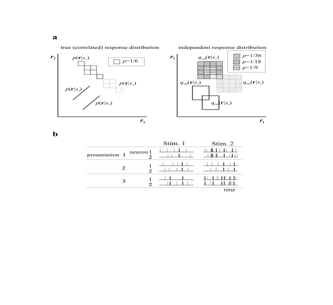
Figure 2: ${\Delta I}$ can be zero when correlations are strong: two hypothetical examples. a. Continuous distributions for four stimuli. The left panel shows the true conditional response distribution. For stimuli 1 and 2 the probability is uniform within each square, and the probability of landing within any one of the squares is 1/6, as indicated in the legend. The lower right square associated with stimulus 1 perfectly overlaps the upper left square associated with stimulus 2; they are offset slightly for clarity. For stimuli 3 and 4 the responses are perfectly correlated: $r_{1}$ perfectly predicts $r_{2}$ and vice-versa. The right panel shows the independent conditional response distribution. For stimuli 1 and 2 the squares now have different probabilities, as indicated in the legend, and none of them are equal to the true probabilities. However, in the overlap region the ratio of the probabilities remains the same and so, via Bayes’ theorem, the responses would be decoded perfectly. For example, assuming uniform priors, if the response fell in the overlap region, under both the true and independent conditional response distributions the probability assigned to stimuli 1 and 2 would be 1/2. For stimuli 3 and 4 the conditional response distributions are now uniform within the rectangles. Note that if a response fell in the overlap region it would not be clear which stimulus caused it. However, under the true distribution the responses never fall in the overlap region, so even if one used the independent conditional response distribution to decode, one would decode perfectly all true responses. b. Spiking response and two stimuli. Synchronous spikes are indicated by thick bars. Stimulus 2 produces a higher firing rate than stimulus 1, but it also produces more synchronous spikes. As is not hard to show, if the probability of synchronous spikes is a function of the firing rates only, and does not depend on the stimulus, then knowledge of synchronous spikes adds no information, and ${\Delta I}$ is zero. Adapted from Nirenberg and Latham, 2003.

An additional example in which correlations exist but do not affect the posterior comes from the linear probabilistic population coding framework [Pouget et al.2003, Ma et al.2006]. In this framework, conditional response distributions have the form

$$p({\bf n}|s)=\phi({\bf n})\exp\big{(}{\bf h}(s)\cdot{\bf n}+\psi(s)\big{)}$$ (7)

where $\phi({\bf n})$ is an arbitrary function of the responses and ${\bf h}(s)$ and $\psi(s)$ are arbitrary functions of the stimulus. Here the correlations, which are contained in $\phi({\bf n})$, could be very complicated, but we don’t have to know them to compute the posterior. As is easy to show,

$$p(s|{\bf n})=\frac{\exp\big{(}{\bf h}(s)\cdot{\bf n}+\psi(s)\big{)}p(s)}{\sum_{s^{\prime}}\exp\big{(}{\bf h}(s^{\prime})\cdot{\bf n}+\psi(s^{\prime})\big{)}p(s^{\prime})}\,,$$ (8)

which is independent of $\phi({\bf n})$, and thus does not require knowledge of the correlations. That we don’t need to know the correlational structure to determine $p(s|{\bf n})$ is not so surprising in this case, since the correlations are stimulus independent. Nevertheless, if this – or a close approximation to it – really is the distribution used by the brain, then we don’t have to worry about correlations at all, even when they are quite strong (i.e., when $\phi({\bf n})$ yields a highly correlated distribution).

7 What experiments tell us

What value of $\Delta I$ does one find in experimental data? The first study to address this question was performed by Yang Dan and colleagues, in the cat lateral geniculate nucleus [Dan et al.1998]. They found that, for some pairs of neurons, using the independent distribution resulted in a 40% information loss. This was not, however, the general trend. Studies in rat barrel cortex [Petersen et al.2001], mouse retina [Nirenberg et al.2001], V1 [Golledge et al.2003], motor cortex [Averbeck and Lee2006] and supplementary motor [Averbeck and Lee2003] area all showed that ${\Delta I}$ was of the order of $10\%$ of the total information. In the one case in which the information loss was measured (as opposed to ${\Delta I}$, which is an upper bound) from experimental data, it was very close to ${\Delta I}$ [Oizumi et al.2008, Oizumi et al.2010].

There is, though, one other study in which large ${\Delta I}$ was found [Ince et al.2010]. In that study, the authors found that for pairs or triplet of neurons in the barrel cortex, ${\Delta I}$ was small. However, by increasing the population size to $8$, ${\Delta I}$ became significant, on the order of $40\%$ of the total information. As the authors note, this could mean that the the neurons receiving input from the barrel cortex must know about the correlations between barrel neurons.

8 What to do when investigating large populations

One problem with ${\Delta I}$ is that it can’t be computed from data for more than a handful of neurons. That’s because it depends on the true conditional response distribution (see Eq. (5)), which we typically don’t know, and, indeed, which the curse of dimensionality tells us we can’t know. What we can do, though, is consider families of parametrized distributions, and ask whether the posterior distribution converges as the family becomes more complex; we just can’t ask if it converges to the true posterior. Two such families commonly used in neuroscience are generalized linear models, or GLMs [Truccolo et al.2005, Pillow et al.2008] and maximum entropy models [Jaynes1957a, Jaynes1957b, Schneidman et al.2003b, Schneidman et al.2006, Shlens et al.2006]. Here we describe them briefly, and summarize what we have learned from them.

Although GLMs and maximum entropy models share some similarities, there are two major differences. The first has to do with bin size. While GLMs are often used with finite bin sizes, this is not necessary, and in fact one of the strengths of these models is that they make sense in the continuous time limit [Gerwinn et al.2010]. For maximum entropy models, on the other hand, results depend critically on bin size [Roudi et al.2009a]. The second difference has to do with how past and current spikes influence the probability of spiking: in GLMs, past spikes have a strong influence and current spikes have none; in maximum entropy models (at least the versions usually used in neuroscience) it is just the opposite.

To make this explicit, we start by writing down the conditional response distribution for GLMs. In these models, the probability of spiking is independent conditioned on the stimulus and previous spikes. Discretizing time (to better make contact with maximum entropy models) and suppressing the dependence on previous spikes (for ease of notation), we have, therefore,

$$q({\bf n}(t)|s)=\prod_{i}q(n_{i}(t)|s)\,.$$ (9)

The individual distributions, $q(n_{i}(t)|s)$, are given by

$$q(n_{i}(t)|s)=\frac{1}{Z}\exp\left[K_{i}[s]n_{i}(t)+\sum_{t^{\prime}<t}h_{i}(t^{\prime})n_{i}(t-t^{\prime})+\sum_{t^{\prime}<t,j\neq i}J_{ij}(t^{\prime})n_{j}(t-t^{\prime})\right]\,.$$ (10)

where $Z$ ensures that $q(n_{i}(t)|s)$ is properly normalized. Here the notation $t^{\prime}<t$ indicates that the sum contains only previous bins (and, recall, time is a discrete variable; thus the sum). This sum, of course, extends only a finite time into the past. The dependence on the stimulus is essentially arbitrary, but it is usually taken to be a temporal linear convolution, or, if the stimulus is spatially varying, a spatio-temporal linear convolution (the brackets around $s$ indicate that there is a dependence on stimulus history). The parameters of the GLM are $h_{i}(t^{\prime})$ and $J_{ij}(t^{\prime})$, and any parameters associated with $K_{i}[s]$. In addition, the nonlinearity does not have to be exponential, but if a different nonlinearity is chosen, extra parameters are (typically) needed to characterize it. And finally, Eq. (10) is technically correct only in the limit of infinitesimally small bin size.

Maximum entropy models are a broad class of models in which one constructs the distribution that has maximum entropy, subject to constraints. Here we consider second order maximum entropy models, since those are the ones most commonly used in neuroscience [Schneidman et al.2006, Shlens et al.2006, Tkačik et al.2006, Tkačik2007, Tang et al.2008, Yu et al.2008, Shlens et al.2009, Roudi et al.2009b, Roudi et al.2009c, Granot-Atdegi et al.2010, Ohiorhenuan et al.2010, Ganmor et al.2011a, Ganmor et al.2011b]. For these models the constraints are on the first and second moments of the probability of spiking in a bin. When those moments can depend on stimulus, the most common form for the model is

$$q({\bf n}(t)|s)=\frac{1}{Z(t)}\exp\left[\sum_{i}h_{i}[s]n_{i}(t)+\sum_{j\neq i}J_{ij}[s]n_{i}(t)n_{j}(t)\right]$$ (11)

where $Z(t)$ ensures that $q({\bf n}|s)$ is properly normalized, and, as above, the fact that the stimulus appears in square brackets in $h_{i}[s]$ and $J_{ij}[t]$ indicates that these terms depend on stimulus history. Equation (11) has the form of the Ising model [Ising1925]; because it also has stimulus dependence, we call it the stimulus-dependent Ising model.

For both GLMs and Ising models, correlations across neurons are contained in the coupling terms, the $J_{ij}$. Thus, one can assess the role of correlations by asking about the quality of the model with and without that term. This is, of course, difficult to do exactly, but one can take an approximate approach. Perhaps the simplest is to build a decoder based on the approximate distribution, $q({\bf n}|s)$, with and without the coupling terms, and either compute its variance numerically or, for discrete stimuli, estimate the probability of making a correct classification. Correlations can then be assessed by comparing the decoder under the two conditions.

So what has been found using these two models? In the case of GLMs, Pillow and colleagues fit the model to retinal ganglion cells from macaque monkeys, and estimated the signal-to-noise ratio with and without the coupling terms [Pillow et al.2008]. A smaller signal to noise ratio essentially means a lower variance decoder. What they found was that, for populations of 27 neurons, the log of the signal to noise was about 20% lower when the coupling terms were excluded from the model (that is, when correlations were ignored). Whether or not one considers this a large or small information loss is a matter of taste; but we feel that it is small – after all, as pointed out by Pillow et al., it’s possible that the ratio of the information with and without the coupling terms could have scaled linearly with the number of neurons. Had this been the case, the information loss would have been on the order of 97%, not 20%. If the information loss stays at 20% for even larger populations, then it may be the case that correlations – or at least pairwise correlations – don’t have much affect on the posterior distribution over stimuli.

For Ising models, most studies have not considered any stimulus dependence [Schneidman et al.2006, Shlens et al.2006, Tkačik2007, Tang et al.2008, Yu et al.2008, Shlens et al.2009, Ganmor et al.2011a]. However, there are four that have [Tkačik2007, Granot-Atdegi et al.2010, Ohiorhenuan et al.2010, Ganmor et al.2011b]. The first of these assumed that the $h_{i}$, but not the $J_{ij}$, depended on the stimulus [Tkačik2007]. For populations of 10 retinal ganglion cells, taking into account the correlations resulted in a modest improvement – the correlated model ($J_{ij}\neq 0$) did about 10% better predicting the absence of firing compared to the independent model ($J_{ij}=0$). The second did not directly examine decoding, but they did find that the stimulus dependent Ising model did a much better job predicting stimuli than the stimulus dependent model [Granot-Atdegi et al.2010]. This was, though, the only model that allowed the couplings, the $J_{ij}$, to depend on stimulus. Interestingly, the dependence was very weak; the implications of that finding are not yet fully understood. In the third model, the authors did not investigate the effect of the coupling terms on the posterior distribution over stimuli [Ohiorhenuan et al.2010]. They did compute information with and without coupling, but, as discussed in the next section (and elsewhere [Latham and Nirenberg2005]), it is not clear what this tells us about the role of correlations. The fourth study was probably the most interesting. Here the authors considered a maximum entropy model that went beyond second order [Ganmor et al.2011b]. When they used that model to decode novel stimuli from $\sim$100 retinal ganglion cells, they could decode them about three times faster than when they used the independent model. Thus, it seems that in this case correlations are clearly important.

9 Other measures of the role of correlations

So far we have asked how correlations affect one’s ability to compute the posterior distribution over stimuli, $p(s|{\bf r})$. However, one may ask a different question: what is the effect of correlations on the ability of a population to encode information? There are several reasons for asking this question. One is to gain intuition about whether correlations are “good” or “bad” – that is, whether they increase or decrease information. The other, related, reason is that the brain might use strategies to modify the correlations, and so measuring correlations in several conditions (e.g., with and without attention) may give us insight into computational strategies used by the brain.

Theoretically, this question was addressed over a decade ago by Abbott and Dayan [Abbott and Dayan1999], who found that correlations can either increase or decrease information in a population code. The reason is rather easy to see, and can be illustrated with only two neurons using a spike count code (in which, for ease of exposition, we pretend that spike count is a continuous variable). Suppose that conditioned on stimulus, the spike counts of the two neurons are positively correlated. In that case, the conditional response distributions form ellipse-like shapes that are neither purely vertical or purely horizontal, as illustrated in Figs. 9.3a and b. The amount of information in the population depends on how easy the responses are to decode, and thus on how much overlap there is between the responses associated with each stimuli. If the mean responses for each of the stimuli are aligned with the long axis of the ellipses, information will be low (correlations decrease information; Fig. 9.3a), and if the mean responses are aligned with the short axis, information will be high (correlations increase information; Fig. 9.3b).

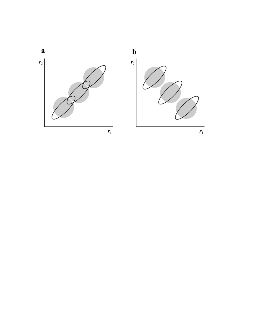
Figure 3: Correlations can either increase or decrease information. In both figures, the responses are taken to be continuous and the conditional response distributions are Gaussian. The ellipses indicate contours containing $90\%$ of the probability for the true responses; the circles contain 90% of the probability for the independent responses. a. Correlations make the responses harder to decode relative to the independent responses, so they decrease information. b. Correlations make the responses easier to decode relative to the independent responses, so they decrease information.

Despite that fact that correlations can either increase or decrease information, there seems to be a feeling among the community that correlations generally decrease it [Zohary et al.1994, Shadlen et al.1996]. While not necessarily true, it would seem to be true whenever neurons have similar tuning properties and neurons are positively correlated (so that the responses look more like Fig. 9.3a than 9.3b). In particular, for a very common correlational structure – neurons with similar tuning are more correlated than neurons with dis-similar tuning curves – increasing correlations does decrease information [Abbott and Dayan1999, Sompolinsky et al.2001] It is this intuition that is behind several studies that looked at how correlations changed with attention. These studies found that attention decreased them, and so, it was stated, information should go up [Cohen and Maunsell2009, Mitchell et al.2009]. However, a recent study showed that if tuning curves do not all have the same amplitude (as is probably the case in the brain), then, even when correlations are large and positive for similarly tuned neurons and weak for dis-similarly tuned ones (exactly the case for which correlations should decrease information), increasing correlations does not lead to much of a decrease in information [Ecker et al.2011]. In fact, for a large enough population, correlations of this type always increase information. So we’re back where we started: correlations can either increase or decrease information, and it can be very hard to make general statements about which one will happen in realistic situations.

10 Correlations, learning and computations: ${\Delta I}$ take 2

Suppose we did an experiment and found that the posterior distribution over stimuli under the independence assumption was equal to the true posterior (${\Delta I}=0$). We could, then, measure single neuron conditional response distributions and use them to build optimal decoders – and, by extension, perform optimal computations. So far in this chapter we have defined this to mean that correlations are not important. However, we should keep in mind that this is not the only notion of important, or even the best one. Indeed, the above assertion comes with a number of caveats.

An important one is the qualifier “optimal” that appears above. While it’s true that when ${\Delta I}=0$ we can decode optimally, it is not true that we can perform approximate decoding optimally. For example, suppose that ${\Delta I}=0$ under the independence assumption, and we wanted to build a linear classifier that divides stimuli into two classes. In Fig. 9.4a we show the responses to eight stimuli, four of which (the ones on the upper left) should be in class 1 and the other four (the ones in the lower right) should be in class 2. Under the independence assumption, in which the conditional response distributions are squares, the optimal linear classifier runs right between the two classes (dashed line). Under the true conditional response distribution, this classifier is always correct for class 2, but correct only about 75% of the time for class 1. This is in contrast to the optimal linear classifier (solid line), for which classification is perfect. However, to find it, the true conditional response distribution must be known. So finding that ${\Delta I}=0$ does not mean one can build an optimal linear classifier.

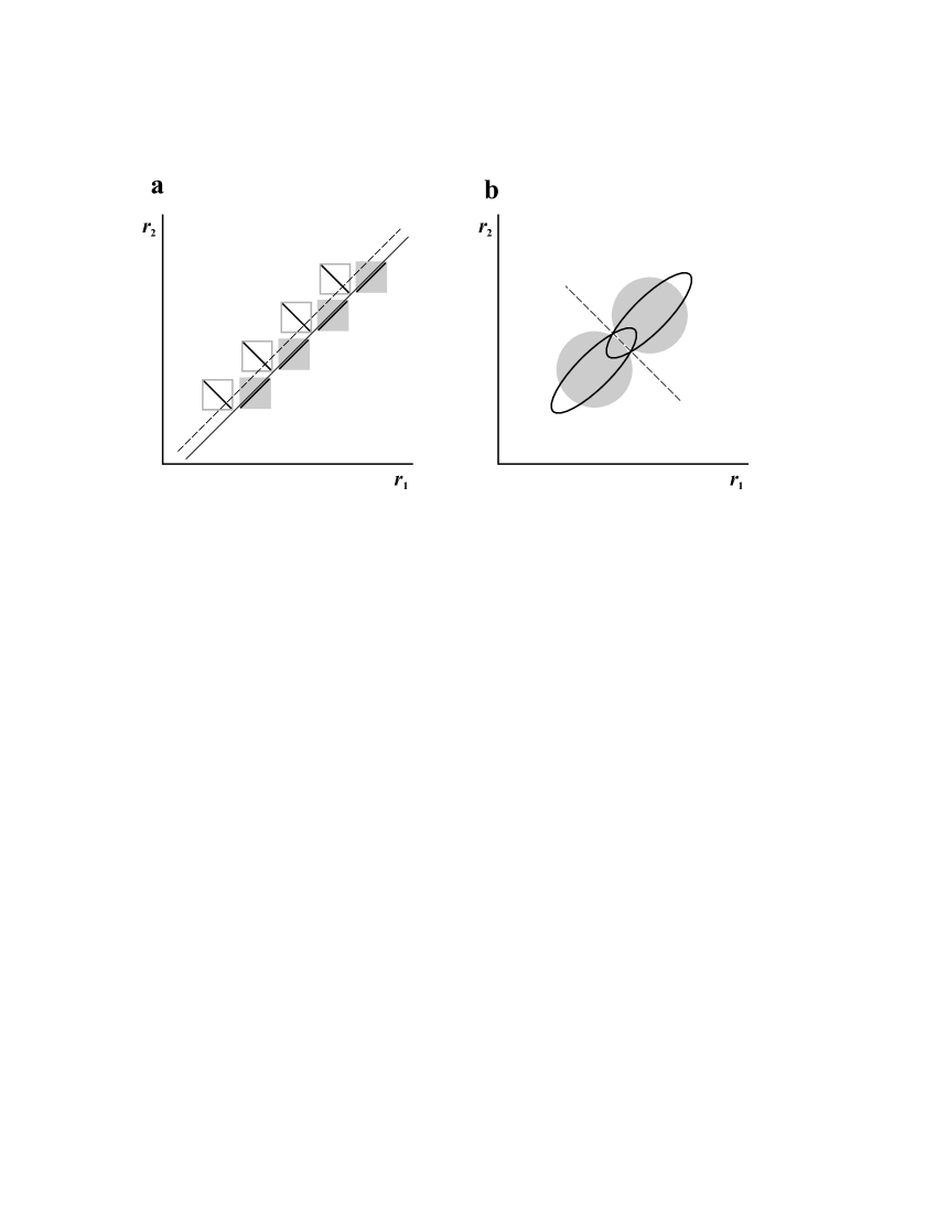
Figure 4: For suboptimal decoders, ${\Delta I}$ can be misleading. a. Eight stimuli need to be divided into two classes using a linear classifier. The responses to the stimuli in class 1 (upper left) are perfectly anti-correlated, as indicated by the bars at $-45^{\circ}$; the responses to stimuli in class 2 (lower right) are perfectly correlated, as indicated by the bars at $+45^{\circ}$. The independent conditional response distributions are squares; open for class 1 and gray for class 2. The dashed line is the optimal linear classifier under the independence assumption, for which some errors are made for class 1 stimuli. The solid line is the optimal linear classifier under the true distribution, for which errors are never made. Thus, although ${\Delta I}=0$, a suboptimal decoder does not perform perfectly. b. Two stimuli need to be divided need into two classes, again with a linear classifier. The ellipses show the true distribution; the circles show the independent one (as in Fig. 9.3). Here ${\Delta I}\neq 0$, since, for almost all responses, the posterior probability of the stimuli is different for the true and independent assumption. However, the linear classifier (dashed line) is the same for both the true and independent distributions. Thus, if all one cared about was the performance of a linear classifier, the fact that ${\Delta I}$ is greater than 0 would be of little interest.

The opposite can also occur: ${\Delta I}$ can be positive even when a suboptimal decoder can work perfectly without knowledge of the correlational structure. Consider, for example Gaussian conditional response distributions from two neurons, as shown in Fig. 9.4b for two stimuli. As is clear from this figure (or is easy to calculate), ${\Delta I}$ is not zero. However, the optimal linear classifier under the independence assumption is the same as it is for the true model.

The take home message here is that ${\Delta I}$ may not be very informative about how well approximate decoders will fare. This is especially important because the problems faced by the brain are so complicated that it almost always (if not always) has to make some approximations. If the approximations the brain makes is known, then finding the correct measure is easy. For example, for a linear classifier, the correct measure would involve a comparison between the fraction correct under the independent conditional response distribution and under the true one. However, if the approximation the brain takes is not known, finding the correct measure is a nontrivial task.

Second, and equally, if not more, important, the brain doesn’t have access to single neuron responses. Thus, even if it wanted to construct the posterior distribution based on the independent responses, it couldn’t. What it sees are the full, correlated responses on every trial. The question we should be asking, then, is: how do correlations affect both learning and the optimal computations used by the network? Pouget and colleagues have addressed the second question, although for a relatively simple problem (by the standards of the brain), cue combination [Ma et al.2006]. Although they did not explicitly consider correlations, the techniques they used could be extended, with some work, in that direction.

11 Summary

So what is the role of correlations? As we have seen here, experimentally one can often construct a near-optimal posterior distribution over stimuli based only on the single neuron conditional response distributions – and, therefore, with no knowledge of the correlational structure [Nirenberg et al.2001, Petersen et al.2001, Averbeck and Lee2003, Golledge et al.2003, Averbeck and Lee2006, Tkačik2007, Granot-Atdegi et al.2010]. There are, though, exceptions [Dan et al.1998, Ince et al.2010, Ganmor et al.2011b]. Of these, the study by Ganmor et al. is especially interesting, because it considered $\sim$100 retinal ganglion cells and found that when correlations were taken into account, decoding speed increased by a factor of about three [Ganmor et al.2011b]. From an evolutionary standpoint, such a speed increase would be highly beneficial. Whether this is a general principle throughout the cortex remains to be seen, but in any case it makes an important point: we should be studying large, not small, neuronal populations.

Finally, our approach – asking whether one needs to know about correlations to accurately represent the outside world – isn’t exactly the question we want to ask of the brain. The brain computes with responses rather than explicitly constructing the posterior distribution, it typically does so using approximate algorithms, and it doesn’t have access to the independent conditional response distribution. The first two are relevant because we saw that when performing approximate computations, it may be necessary to know the true distribution even when ${\Delta I}=0$ (Fig. 9.4a), and it may not be necessary to know the true distribution even when ${\Delta I}\neq 0$ (Fig. 9.4b). The third is relevant because the brain has to learn what to do based on correlated responses, and so the real question is: how do correlations affect learning? This is a problem for which the answer is not known, at least not in general. Thus, despite much work on the role of correlations, much is left to be done.

12 Acknowledgments

We would like to thank Jonathan Pillow for valuable feedback on this chapter.

References

- [\citeauthoryearAbbott and Dayan1999] Abbott LF, Dayan P (1999) The effect of correlated variability on the accuracy of a population code. Neural Comput 11:91–101.
- [\citeauthoryearAmari and Nakahara2006] Amari S, Nakahara H (2006) Correlation and independence in the neural code. Neural Comput 18:1259–1267.
- [\citeauthoryearAverbeck and Lee2003] Averbeck BB, Lee D (2003) Neural noise and movement-related codes in the macaque supplementary motor area. J Neurosci 23:7630–7641.
- [\citeauthoryearAverbeck and Lee2006] Averbeck BB, Lee D (2006) Effects of noise correlations on information encoding and decoding. J Neurophysiol 95:3633–3644.
- [\citeauthoryearBair et al.2001] Bair W, Zohary E, Newsome WT (2001) Correlated firing in macaque visual area MT: time scales and relationship to behavior. J Neurosci 21:1676–1697.
- [\citeauthoryearBialek and Rieke1992] Bialek W, Rieke F (1992) Reliability and information transmission in spiking neurons. Trends Neurosci 15:428–434.
- [\citeauthoryearBialek et al.1991] Bialek W, Rieke F, de Ruyter van Steveninck RR, Warland D (1991) Reading a neural code. Science 252:1854–1857.
- [\citeauthoryearChater et al.2006] Chater N, Tenenbaum JB, Yuille A (2006) Probabilistic models of cognition: where next? Trends Cogn Sci 10:292–293.
- [\citeauthoryearCohen and Kohn2011] Cohen MR, Kohn A (2011) Measuring and interpreting neuronal correlations. Nat Neurosci 14:811–819.
- [\citeauthoryearCohen and Maunsell2009] Cohen MR, Maunsell JH (2009) Attention improves performance primarily by reducing interneuronal correlations. Nat Neurosci 12:1594–1600.
- [\citeauthoryearCover and Thomas1991] Cover T, Thomas J (1991) Elements of Information theory. New York: Wiley.
- [\citeauthoryearDan et al.1998] Dan Y, Alonso JM, Usrey WM, Reid RC (1998) Coding of visual information by precisely correlated spikes in the LGN. Nature Neurosci 1:501–507.
- [\citeauthoryearDeger et al.2011] Deger M, Helias M, Boucsein C, Rotter S (2011) Statistical properties of superimposed stationary spike trains. J Comp Neurosci in press.
- [\citeauthoryearEcker et al.2011] Ecker A, Berens P, Tolias A, Bethge M (2011) The effect of noise correlations in populations of diversely tuned neurons. J Neurosci in press.
- [\citeauthoryearErnst and Banks2002] Ernst MO, Banks MS (2002) Humans integrate visual and haptic information in a statistically optimal fashion. Nature 415:429–433.
- [\citeauthoryearEskandar et al.1992] Eskandar EN, Richmond BJ, Optican LM (1992) Role of inferior temporal neurons in visual memory. I. temporal encoding of information about visual images, recalled images, and behavioral context. J Neurophysiol 68:1277–1295.
- [\citeauthoryearGanmor et al.2011a] Ganmor E, Segev R, Schneidman E (2011a) The architecture of functional interaction networks in the retina. J Neurosci 31:3044–3054.
- [\citeauthoryearGanmor et al.2011b] Ganmor E, Segev R, Schneidman E (2011b) Sparse low-order interaction network underlies a highly correlated and learnable neural population code. Proc Natl Acad Sci USA 108:9679–9684.
- [\citeauthoryearGawne et al.1996] Gawne TJ, Kjaer TW, Hertz JA, Richmond BJ (1996) Adjacent visual cortical complex cells share about 20% of their stimulus-related information. Cereb Cortex 6:482–489.
- [\citeauthoryearGawne and Richmond1993] Gawne TJ, Richmond BJ (1993) How independent are the messages carried by adjacent inferior temporal cortical neurons? J Neurosci 13:2758–2771.
- [\citeauthoryearGerwinn et al.2010] Gerwinn S, Macke JH, Bethge M (2010) Bayesian inference for generalized linear models for spiking neurons. Front Comput Neurosci 4.
- [\citeauthoryearGolledge et al.2003] Golledge HD, Panzeri S, Zheng F, Pola G, Scannell W, Giannikopoulos DV, Mason RJ, Tovee MJ, Young MP (2003) Correlations, feature-binding and population coding in primary visual cortex. Neuroreport 14:1045–1050.
- [\citeauthoryearGranot-Atdegi et al.2010] Granot-Atdegi E, Tkačik G, Segev R, Schneidman E (2010) A stimulus-dependent maximum entropy model of the retinal population neural code In Frontiers in Neuroscience. Computational and Systems Neuroscience 2010.
- [\citeauthoryearGray1999] Gray C (1999) The temporal correlation hypothesis of visual feature integration: still alive and well. Neuron 24:31–47, 111–125.
- [\citeauthoryearInce et al.2010] Ince R, Senatore R, Arabzadeh E, Montani F, E. DM, Panzeri S (2010) Information-theoretic methods for studying population codes. Neural Networks 23:713–727.
- [\citeauthoryearIsing1925] Ising E (1925) Beitrag zur theorie des ferromagnetismus. Z Physik 31:253–258.
- [\citeauthoryearJacobs1999] Jacobs RA (1999) Optimal integration of texture and motion cues to depth. Vision Res 39:3621–3629.
- [\citeauthoryearJaynes1957a] Jaynes ET (1957a) Information theory and statistical mechanics. Physical Review Series II 106:620–630.
- [\citeauthoryearJaynes1957b] Jaynes ET (1957b) Information theory and statistical mechanics II. Physical Review Series II 108:171–190.
- [\citeauthoryearKayser et al.2010] Kayser C, Logothetis NK, Panzeri S (2010) Millisecond encoding precision of auditory cortex neurons. Proc Natl Acad Sci USA 107:16976–16981.
- [\citeauthoryearKim et al.1990] Kim DO, Sirianni JG, Chang SO (1990) Responses of DCN-PVCN neurons and auditory nerve fibers in unanesthetized decerebrate cats to AM and pure tones: analysis with autocorrelation/power-spectrum. Hear Res 45:95–113.
- [\citeauthoryearKörding and Wolpert2004] Körding KP, Wolpert DM (2004) Bayesian integration in sensorimotor learning. Nature 427:244–247.
- [\citeauthoryearKullback and Leibler1951] Kullback S, Leibler R (1951) On information and sufficiency. Annals of Mathematical Statistics 22:79–86.
- [\citeauthoryearLatham and Nirenberg2005] Latham PE, Nirenberg S (2005) Synergy, redundancy, and independence in population codes, revisited. J Neurosci 25:5195–5206.
- [\citeauthoryearLondon et al.2010] London M, Roth A, Beeren L, Hausser M, Latham PE (2010) Sensitivity to perturbations in vivo implies high noise and suggests rate coding in cortex. Nature 466:123–127.
- [\citeauthoryearMa et al.2006] Ma WJ, Beck JM, Latham PE, Pouget A (2006) Bayesian inference with probabilistic population codes. Nat Neurosci 9:1432–1438.
- [\citeauthoryearMa et al.2011] Ma WJ, Navalpakkam V, Beck JM, Berg R, Pouget A (2011) Behavior and neural basis of near-optimal visual search. Nat Neurosci 14:783–790.
- [\citeauthoryearMarmarelis and Marmarelis1978] Marmarelis P, Marmarelis V (1978) Analysis of Physiological Systems: The White-Noise Approach Plenum, New York.
- [\citeauthoryearMastronarde1983a] Mastronarde DN (1983a) Correlated firing of cat retinal ganglion cells. I. Spontaneously active inputs to X- and Y-cells. J Neurophysiol 49:303–324.
- [\citeauthoryearMastronarde1983b] Mastronarde DN (1983b) Correlated firing of cat retinal ganglion cells. II. Responses of X- and Y-cells to single quantal events. J Neurophysiol 49:325–349.
- [\citeauthoryearMilner1974] Milner P (1974) A model for visual shape recognition. Psychol Rev 81:521–535.
- [\citeauthoryearMitchell et al.2009] Mitchell JF, Sundberg KA, Reynolds JH (2009) Spatial attention decorrelates intrinsic activity fluctuations in macaque area V4. Neuron 63:879–888.
- [\citeauthoryearNirenberg et al.2001] Nirenberg S, Carcieri SM, Jacobs AL, Latham PE (2001) Retinal ganglion cells act largely as independent encoders. Nature 411:689–701.
- [\citeauthoryearNirenberg and Latham2003] Nirenberg S, Latham PE (2003) Decoding neuronal spike trains: How important are correlations? Proc Natl Acad Sci USA 100:7348–7353.
- [\citeauthoryearOhiorhenuan et al.2010] Ohiorhenuan IE, Mechler F, Purpura KP, Schmid AM, Hu Q, Victor JD (2010) Sparse coding and high-order correlations in fine-scale cortical networks. Nature 466:617–621.
- [\citeauthoryearOizumi et al.2010] Oizumi M, Ishii T, Ishibashi K, Hosoya T, Okada M (2010) Mismatched decoding in the brain. J Neurosci 30:4815–4826.
- [\citeauthoryearOizumi et al.2008] Oizumi M, Ishii T, Ishibashi K, Hosoya T, Okada M (2008) A general framework for investigating how far the decoding process in the brain can be simplified In Koller D, Schuurmans D, Bengio Y, Bottou L, editors, Advances in Neural Information Processing Systems 21, pp. 1225–1232.
- [\citeauthoryearOptican and Richmond1987] Optican LM, Richmond BJ (1987) Temporal encoding of two-dimensional patterns by single units in primate inferior temporal cortex. III. information theoretic analysis. J Neurophysiol 57:162–178.
- [\citeauthoryearPetersen et al.2001] Petersen RS, Panzeri S, Diamond ME (2001) Population coding of stimulus location in rat somatosensory cortex. Neuron 32:503–514.
- [\citeauthoryearPillow et al.2008] Pillow JW, Shlens J, Paninski L, Sher A, Litke AM, Chichilnisky EJ, Simoncelli EP (2008) Spatio-temporal correlations and visual signalling in a complete neuronal population. Nature 454:995–999.
- [\citeauthoryearPouget et al.2003] Pouget A, Dayan P, Zemel RS (2003) Inference and computation with population codes. Annu Rev Neurosci 26:381–410.
- [\citeauthoryearRichmond and Optican1990] Richmond BJ, Optican LM (1990) Temporal encoding of two-dimensional patterns by single units in primate primary visual cortex. II. Information transmission. J Neurophysiol 64:370–380.
- [\citeauthoryearRodieck1967] Rodieck R (1967) Maintained activity of cat retinal ganglion cells. J Neurophysiol 30:1043–1071.
- [\citeauthoryearRoudi et al.2009a] Roudi Y, Nirenberg S, Latham PE (2009a) Pairwise maximum entropy models for studying large biological systems: when they can work and when they can’t. PLoS Comput Biol 5:e1000380.
- [\citeauthoryearRoudi et al.2009b] Roudi Y, Tyrcha J, Hertz J (2009b) Ising model for neural data: Model quality and approximate methods for extracting functional connectivity. Phys. Rev. E 79:051915.
- [\citeauthoryearRoudi et al.2009c] Roudi Y, Aurell E, Hertz JA (2009c) Statistical physics of pairwise probability models. Front. Comput. Neurosci. 3:22.
- [\citeauthoryearSchneidman et al.2006] Schneidman E, Berry M, Segev R, Bialek W (2006) Weak pairwise correlations imply strongly correlated network states in a neural population. Nature 440:1007–1012.
- [\citeauthoryearSchneidman et al.2003a] Schneidman E, Bialek W, Berry MJ (2003a) Synergy, redundancy, and independence in population codes. J Neurosci 23:11539–11553.
- [\citeauthoryearSchneidman et al.2003b] Schneidman E, Still S, Berry MJ, Bialek W (2003b) Network information and connected correlations. Phys Rev Lett 91:238701–238701.
- [\citeauthoryearShadlen et al.1996] Shadlen MN, Britten KH, Newsome WT, Movshon JA (1996) A computational analysis of the relationship between neuronal and behavioral responses to visual motion. J Neurosci 16:1486–1510.
- [\citeauthoryearShannon and Weaver1949] Shannon C, Weaver W (1949) The mathematical theory of communication University of Illinois Press, Urbana, Illinois.
- [\citeauthoryearShlens et al.2009] Shlens J, Field GD, Gauthier JL, Greschner M, Sher A, Litke AM, Chichilnisky EJ (2009) The structure of large-scale synchronized firing in primate retina. J Neurosci 29:5022–5031.
- [\citeauthoryearShlens et al.2006] Shlens J, Field G, Gauthier J, Grivich M, Petrusca D, Sher A, Litke A, Chichilnisky E (2006) The structure of multi-neuron firing patterns in primate retina. J Neurosci 26:8254–8266.
- [\citeauthoryearSompolinsky et al.2001] Sompolinsky H, Yoon H, Kang K, Shamir M (2001) Population coding in neuronal systems with correlated noise. Phys. Rev. E 64:051904.
- [\citeauthoryearStaude et al.2010] Staude B, Grün S, Rotter S (2010) Higher-order correlations in non-stationary parallel spike trains: statistical modeling and inference. Front Comput Neurosci 4.
- [\citeauthoryearTang et al.2008] Tang A, Jackson D, Hobbs J, Chen W, Smith JL, Patel H, Prieto A, Petrusca D, Grivich MI, Sher A, Hottowy P, Dabrowski W, Litke AM, Beggs JM (2008) A maximum entropy model applied to spatial and temporal correlations from cortical networks in vitro. J Neurosci 28:505–518.
- [\citeauthoryearTkačik2007] Tkačik G (2007) Information flow in biological networks. Ph.D. diss., Princeton University.
- [\citeauthoryearTkačik et al.2006] Tkačik G, Schneidman E, Berry M, Bialek W (2006) Ising models for networks of real neurons. arXiv:q-bio/0611072v1 .
- [\citeauthoryearTruccolo et al.2005] Truccolo W, Eden U, Fellows M, Donoghue J, Brown E (2005) A point process framework for relating neural spiking activity to spiking history, neural ensemble and extrinsic covariate effects. J Neurophys 93:1074–1089.
- [\citeauthoryearVictor2005] Victor JD (2005) Spike train metrics. Current Opinion in Neurobiology 15:585–592.
- [\citeauthoryearVictor and Purpura1996] Victor JD, Purpura KP (1996) Nature and precision of temporal coding in visual cortex: a metric-space analysis. J Neurophysiol 76:1310–1326.
- [\citeauthoryearvon der Malsburg1981] von der Malsburg C (1981) The correlation theory of brain function. MPI Biophysical Chemistry, Internal Report 81–2 .
- [\citeauthoryearWiener and Richmond1999] Wiener MC, Richmond BJ (1999) Using response models to estimate channel capacity for neuronal classification of stationary visual stimuli using temporal coding. J Neurophysiol 82:2861–2875.
- [\citeauthoryearWu et al.2001] Wu S, Nakahara H, Amari S (2001) Population coding with correlation and an unfaithful model. Neural Comput 13:775–797.
- [\citeauthoryearWu et al.2000] Wu S, Nakahara H, Murata N, Amari S (2000) Population decoding based on an unfaithful model In Advances in neural information processing systems, pp. 167–173, Cambridge, MA: MIT press.
- [\citeauthoryearYu et al.2008] Yu S, Huang D, Singer W, Nikolic D (2008) A small world of neuronal synchrony. Cereb Cortex 18:2891–2901.
- [\citeauthoryearZohary et al.1994] Zohary E, Shadlen MN, Newsome WT (1994) Correlated neuronal discharge rate and its implications for psychophysical performance. Nature 370:140–143.