A test for Archimedeanity in bivariate copula models

Abstract

We propose a new test for the hypothesis that a bivariate copula is an Archimedean copula. The test statistic is based on a combination of two measures resulting from the characterization of Archimedean copulas by the property of associativity and by a strict upper bound on the diagonal by the Fréchet-upper bound. We prove weak convergence of this statistic and show that the critical values of the corresponding test can be determined by the multiplier bootstrap method. The test is shown to be consistent against all departures from Archimedeanity if the copula satisfies weak smoothness assumptions. A simulation study is presented which illustrates the finite sample properties of the new test.

Keywords and Phrases: Archimedean Copula, associativity, functional delta method, multiplier bootstrap
AMS Subject Classification: Primary 62G10 ; secondary 62G20

1 Introduction

Let $F$ be a bivariate continuous distribution function with marginal distribution functions $F_{1}$ and $F_{2}$. By Sklar’s Theroem [see Sklar, (1959)] we can decompose $F$ as follows

$$F(\mathbf{x})=C(F_{1}(x_{1}),F_{2}(x_{2})),\quad\mathbf{x}=(x_{1},x_{2})\in\mathbb{R}^{2},$$ (1.1)

where $C$ is the unique copula associated to $F$. By definition, $C$ is a bivariate distribution function on the unit square $[0,1]^{2}$ whose univariate marginals are standard uniform distributions on the interval $[0,1]$. Equation (1.1) is usually interpreted in the way that the copula $C$ completely characterizes the information about the stochastic dependence contained in $F$. For an extensive exposition on the theory of copulas we refer the reader to the monograph Nelsen, (2006).

In the last decades, various parametric models for copulas have been developed, among which the class of Archimedean copulas forms one the most famous and largest class, see Genest and MacKay, (1986); Nelsen, (2006); McNeil and Nešlehová, (2009) among many others. Many widely used copulas, such as Clayton-, Gumbel- and Frank-copulas are in fact Archimedean copulas. The elements of this class may be characterized by a continuous, strictly decreasing and convex function $\Phi:[0,1]\rightarrow[0,\infty]$ satisfying $\Phi(1)=0$ such that

$$C(\mathbf{u})=\Phi^{[-1]}\left[\Phi(u_{1})+\Phi(u_{2})\right]\quad\text{for all }\mathbf{u}=(u_{1},u_{2})\in[0,1]^{2}.$$

The function $\Phi$ is called the generator of $C$ and its pseudo-ineverse $\Phi^{[-1]}(t)$ is defined as the usual inverse $\Phi^{-1}(t)$ for $t\in[0,\Phi(0)]$ and is set to $0$ for $t\geq\Phi(0)$. The prominence of the class of Archimedean copulas basically stems from the fact that they are easy to handle and to simulate, see Genest et al., (2011). While the estimation of Archimedean copulas has been investigated in Genest and Rivest, (1993) and recently more thoroughly in Genest et al., (2011), the issue of testing for the hypothesis that the copula is an Archimedean one has found much less interest in the literature. The present paper fills this gap by developing a consistent test for this hypothesis.

Our interest in this problem stems from recent work of Genest and Rivest, (1993), Wang and Wells, (2000) and Naifar, (2011) who proposed Archimedean copulas for modeling dependencies between bivariate observations (among many others). We also refer to the work of Rivest and Wells, (2001) who used Archimedean copulas for modeling the dependence in the context of censored data.

To the best of our knowledge, the only available test hitherto has been discussed in Jaworski, (2010). This author proposed a procedure which is based on a characterization of Archimedean copulas similar to the one stated in Theorem 4.1.6 in Nelsen, (2006) [which dates back to Ling, (1965)]. To be precise recall that a bivariate copula $C$ is called associative if and only if the identity

$$C(x,C(y,z))=C(C(x,y),z)\quad$$ (1.2)

holds for all $(x,y,z)\in[0,1]^{3}.$ Theorem 4.1.6 in Nelsen, (2006) shows that a bivariate copula $C$ is an Archimedean copula if and only if $C$ is associative and the inequality $C(u,u)<u$ holds for all $u\in(0,1)$, i.e. on the diagonal $C$ is strictly dominated by the Fréchet-upper bound $M(\mathbf{u})=\min(u_{1},u_{2})$. The procedure suggested in Jaworski, (2010) is in fact to test for associativity in order to check the validity of an Archimedean copula model. The corresponding test statistic is defined as

$$\mathcal{T}_{n}(x,y)=\sqrt{n}(C_{n}(x,C_{n}(y,y))-C_{n}(C_{n}(x,y),y),$$

where $(x,y)$ is some fixed point in the open cube $(0,1)^{2}$ and $C_{n}$ denotes the empirical copula, see Section 2 for details. The main advantage of this approach is its simplicity, in particular the simple limit distribution of the resulting test statistic, which is in fact normal. On the other hand this simplicity has its price in terms of consistency. In our opinion, the method proposed by Jaworski, (2010) has at least three mayor drawbacks. First of all, it is clearly not consistent against a large class of alternatives since it only tests for equation (1.2) with $y=z$. Second, Jaworski, (2010) uses a pointwise approach in order to test for a global hypothesis as in (1.2). This means that the test may not reject the hypothesis because (1.2) is satisfied at the particular point $(x,y,y)$ under investigation, although there may exist many other points where (1.2) is not satisfied. Third, there exist copulas which are in fact associative but not Archimedean. These problems also have strong implications for the practical applicability of the test as demonstrated by results in a simulation study in Jaworski, (2010), where the sample size has to be chosen extremely large in order to get reasonable rejection probabilities.

To the best of our knowledge there exists no test for an Archimedean copula, which is consistent against general alternatives and it is the primary purpose of this paper to develop such a procedure and to investigate its statistical properties. We propose a test statistic which is based on a combination of two measures resulting from the characterization of Archimedean copulas, namely the property of associativity as described in (1.2) and the strict upper bound on the diagonal $C(u,u)<u$ for all $u\in(0,1)$. In Section 2 we define a new process which is based on an estimate of the difference of the left and right hand side of the defining equation (1.2) for associativity. We prove weak convergence of this process in the space of all uniformly bounded functions on the cube $[0,1]^{3}$. As a consequence, we also obtain weak convergence of a corresponding Cramér-von-Mises and a Kolmogorov-Smirnov type statistic. Because the asymptotic distribution depends in a complicated manner on the underlying copula we propose a multiplier bootstrap procedure to obtain the critical values and show its validity. As a first main result we obtain a test for associativity, which is consistent against all alternatives satisfying weak smoothness assumptions on $C$. In Section 3 we utilize these findings to develop an asymptotic test for the hypothesis of Archimedeanity. Finally in Section 4 we investigate the finite sample performance of the new test by means of a simulation study.

2 Testing Associativity

2.1 The test statistic and its asymptotic behavior

In the following let $\mathbf{X}_{1},\dots,\mathbf{X}_{n}$, $\mathbf{X}_{i}=(X_{i1},X_{i2})$ denote independent identically distributed bivariate random vectors with continuous distribution function $F$, marginal distribution functions $F_{1}$ and $F_{2}$ and copula $C=F(F_{1}^{-},F_{2}^{-})$. In this paragraph we will introduce a test statistic for the null hypothesis that the underlying copula is associative, i.e. $C$ satisfies condition (1.2) for all $(x,y,z)\in[0,1]^{3}$.

For this purpose we briefly summarize relevant notations and results on the empirical copula, which is the simplest and most popular nonparametric estimator of the copula. In particular we define the empirical copula by

$$C_{n}(\mathbf{u})=F_{n}(F_{n1}^{-}(u_{1}),F_{n2}^{-}(u_{2})),$$

where $F_{n}(\mathbf{x})=n^{-1}\sum_{i=1}^{n}\mathbb{I}\{\mathbf{X}_{i}\leq\mathbf{x}\}$ and $F_{np}(x_{p})=n^{-1}\sum_{i=1}^{n}\mathbb{I}\{X_{ip}\leq x_{p}\},p=1,2$ are the joint and marginal empirical distribution functions of the sample $\mathbf{X}_{1},\dots,\mathbf{X}_{n}$, respectively. It is a well known result that under the assumptions of continuous partial derivatives of $C$ the corresponding empirical copula process

$$\mathbb{C}_{n}=\sqrt{n}(C_{n}-C)$$ (2.1)

converges weakly towards a Gaussian limit field $\mathbb{G}_{C}$ in $l^{\infty}([0,1]^{2})$, see Rüschendorf, (1976); Fermanian et al., (2004); Tsukahara, (2005) among others. Defining $\dot{C}_{p}$ as the $p$-th partial derivative of $C$ ($p=1,2$) the process $\mathbb{G}_{C}$ can be expressed as

$$\mathbb{G}_{C}(\mathbf{x})=\mathbb{B}_{C}(\mathbf{x})-\dot{C}_{1}(\mathbf{x})\mathbb{B}_{C}(x_{1},1)-\dot{C}_{2}(\mathbf{x})\mathbb{B}_{C}(1,x_{2})$$ (2.2)

with the copula-brownian bridge $\mathbb{B}_{C}$, i.e. $\mathbb{B}_{C}$ is a centered Gaussian field with $\operatorname{Cov}(\mathbb{B}_{C}(\mathbf{x}),\mathbb{B}_{C}(\mathbf{y}))=C(\mathbf{x}\wedge\mathbf{y})-C(\mathbf{x})C(\mathbf{y})$, where the minimum of two vectors is defined component-wise. As explained in Segers, (2011) the assumption of continuity of the partial derivatives of $C$ on the whole unit square does not hold for many (even most) commonly used copula models and as a consequence Segers provides the result that the following nonrestrictive smoothness condition is sufficient in order to obtain weak convergence of the empirical copula process defined in (2.1).

Condition 2.1.

For $p=1,2$ the first order partial derivative $\dot{C}_{p}$ of the copula $C$ with respect to $x_{p}$ exists and is continuous on the set $V_{p}=\{\mathbf{u}\in[0,1]^{2}\,:\,0<u_{p}<1\}$.

Now, in order to test for associativity we consider the process

$$\mathbb{H}_{n}(x,y,z)=\sqrt{n}\left\{C_{n}(x,C_{n}(y,z))-C_{n}(C_{n}(x,y),z)\right\},$$

where $(x,y,z)\in[0,1]^{3}$. The asymptotic properties of the process $\{\mathbb{H}_{n}(x,y,z)\}_{(x,y,z)\in[0,1]^{3}}$ are summarized in the following Theorem. Throughout this paper $l^{\infty}(T)$ denotes the set of all uniformly bounded functions on $T$, and the symbol $\ \rightsquigarrow\$ denotes uniform convergence in a metric space (which will be specified in the corresponding statements).

Theorem 2.2.

If the copula $C$ is associative and satisfies Condition 2.1, then it holds

$$\mathbb{H}_{n}\ \rightsquigarrow\ \mathbb{H}_{C}\quad\text{ in }~{}~{}l^{\infty}([0,1]^{3}),$$

where the limit field $\mathbb{H}_{C}$ can be expressed as

$$\mathbb{H}_{C}(x,y,z)=\mathbb{G}_{C}(x,C(y,z))-\mathbb{G}_{C}(C(x,y),z)+\dot{C}_{2}(x,C(y,z))\mathbb{G}_{C}(y,z)-\dot{C}_{1}(C(x,y),z)\mathbb{G}(x,y).$$

Proof. If the copula $C$ is associative we can write the process $\mathbb{H}_{n}$ as

$$\mathbb{H}_{n}=\sqrt{n}\left\{\Phi(C_{n})-\Phi(C)\right\},$$

where the functional $\Phi:\mathbb{D}_{\Phi}\rightarrow l^{\infty}([0,1]^{3})$ is defined for

$$\alpha\in\mathbb{D}_{\Phi}=\{F:F\text{ cdf on }[0,1]^{2}\}$$

by

$$\Phi(\alpha)(x,y,z)=\alpha(x,\alpha(y,z))-\alpha(\alpha(x,y),z).$$

We will show later that under Condition 2.1 the mapping $\Phi$ is Hadamard-differentiable at $C$ tangentially to the space

$$\mathbb{D}_{0}=\left\{\gamma\in C[0,1]^{2}\,|\,\gamma(\mathbf{u})=0\text{ for all }\,\mathbf{u}\in[0,1]^{2}\text{ s.t. }C(\mathbf{u})\in\{0,1\}\right\},$$

with derivative given by

$$\Phi_{C}^{\prime}(\alpha)(x,y,z)=\alpha(x,C(y,z))-\alpha(C(x,y),z)+\dot{C}_{2}(x,C(y,z))\alpha(y,z)-\dot{C}_{1}(C(x,y),z)\alpha(x,y).$$

Observing that $\mathbb{B}_{C}\in\mathbb{D}_{0}$ a.s., the functional delta method, see Theorem 3.9.4 in Van der Vaart and Wellner, (1996), yields the assertion.

We now briefly sketch how to see the Hadamard-differentiability of the mapping $\Phi$: let $t_{n}\rightarrow 0$ and $\alpha_{n}\in l^{\infty}([0,1]^{2})$ with $\alpha_{n}\rightarrow\alpha\in\mathbb{D}_{0}$ such that $C+t_{n}\alpha_{n}\in\mathbb{D}_{\Phi}$. Then

$$t_{n}^{-1}\{\Phi(C+t_{n}\alpha_{n})-\Phi(C)\}=L_{n1}+L_{n2}-L_{n3}$$

where

$$L_{n1}(x,y,z) =\alpha_{n}(x,(C+t_{n}\alpha_{n})(y,z))-\alpha_{n}((C+t_{n}\alpha_{n})(x,y),z)$$

$$L_{n2}(x,y,z) =t_{n}^{-1}\{C(x,(C+t_{n}\alpha_{n})(y,z))-C(x,C(y,z))\}$$

$$L_{n3}(x,y,z) =t_{n}^{-1}\{C((C+t_{n}\alpha_{n})(x,y),z)-C(C(x,y),z)\}.$$

Exploiting the fact that $\alpha_{n}$ converges uniformly to a bounded function and that $\alpha$ is uniformly continuous one can conclude that $L_{n1}(x,y,z)=\alpha(x,C(y,z))-\alpha(C(x,y),z)+o(1)$ uniformly in $(x,y,z)\in[0,1]^{3}$. Regarding the summand $L_{n2}$ we have to split the investigation in two cases. First, we consider all those $(x,y,z)\in[0,1]^{3}$ for which $C(y,z)\in(0,1)$. A Taylor expansion of $C(x,\cdot)$ at $C(y,z)$ yields

$$L_{n2}(x,y,z)=\dot{C}_{2}(x,C(y,z))\alpha_{n}(y,z)+r_{n}(x,y,z),$$

where the error term can be written as

$$r_{n}(x,y,z)=\big{(}\dot{C}_{2}(x,u_{n})-\dot{C}_{2}(x,C(y,z))\big{)}\alpha_{n}(y,z)$$

with some intermediate point $u_{n}$ between $C(y,z)$ and $(C+t_{n}\alpha_{n})(y,z)$. The main term uniformly converges to $\dot{C}_{2}(x,C(y,z))\alpha(y,z)$ [note that partial derivatives of copulas are uniformly bounded by $1$] and it remains to show that $r_{n}(x,y,z)=o(1)$ uniformly in $(x,y,z)$ with $C(y,z)\in(0,1)$.

To see this, we will show at the end of this proof that for any $\varepsilon>0$ there exists a $\delta>0$, such that

$$\limsup_{n\rightarrow\infty}\sup_{\mathbf{v}\in A_{\delta}}|\alpha_{n}(\mathbf{v})|\leq\varepsilon.$$ (2.3)

where $\mathbf{v}=(y,z)$, $A_{\delta}=\{\mathbf{v}\in[0,1]^{2}|\ C(\mathbf{v})\in[0,\delta)\cup(1-\delta,1]\}$. Then, since partial derivatives of copulas are bounded by $1$, we can conclude that

$$\limsup_{n\rightarrow\infty}\sup_{x\in[0,1],(y,z)\in A_{\delta}}|r_{n}(x,y,z)|\leq\varepsilon.$$

Due to Condition 2.1 the partial derivative $\dot{C}_{2}$ is uniformly continuous on the quadrangle $[0,1]\times[\delta,1-\delta]$. Thus, since $\alpha$ is uniformly bounded and since $u_{n}\rightarrow C(y,z)$, we obtain uniform convergence of $r_{n}(x,y,z)$ to $0$ for all $(y,z)$ s.t. $C(y,z)\in[\delta,1-\delta]$, i.e. for $(y,z)\in[0,1]^{2}\setminus A_{\delta}$. Combining the two facts derived above, it follows that

$$\limsup_{n\rightarrow\infty}\sup_{x\in[0,1],C(y,z)\in(0,1)}|r_{n}(x,y,z)|\leq\varepsilon.$$

Since $\varepsilon>0$ was arbitrary, this $\limsup$ must be zero. Summarizing, the case $(x,y,z)\in[0,1]^{3}$ such that $C(y,z)\in(0,1)$ is finished.

In the remaining case $C(y,z)\in\{0,1\}$, i.e. $(y,z)\in A_{0}$, Lipschitz-continuity of $C$ entails that

$$|L_{n2}(x,y,z)|=t_{n}^{-1}|C(x,C(y,z)+t_{n}\alpha_{n}(y,z))-C(x,C(y,z))|\leq\alpha_{n}(y,z)=\alpha(y,z)+o(1)=o(1)$$

uniformly in $(x,y,z)$ since in this case $\alpha(y,z)=0$. Finally, the summand $L_{n3}$ may be treated analogously.

To complete the proof it remains to show (2.3). Exploiting uniform convergence of $\alpha_{n}$, uniform continuity of $\alpha$ and the fact that $\alpha(\mathbf{v})=0$ for all $\mathbf{v}\in A_{0}=\{\mathbf{v}\,|\,C(\mathbf{v})\in\{0,1\}\}$, we can conclude that there exists a $\kappa>0$ such that $|\alpha_{n}(\mathbf{v})|\leq\varepsilon$ for all $\mathbf{v}\in A_{0}^{\kappa}=\{\mathbf{v}\,|\,\exists\,\mathbf{u}\in A_{0}\text{ s.t. }\|\mathbf{u}-\mathbf{v}\|\leq\kappa\}$ and sufficiently large $n$. For $v_{1}\in[\kappa,1]$ let $\delta(v_{1})=\sup\{C(v_{1},z)\,|\,(v_{1},z)\in A_{0}^{\kappa}\}$ [which equals $C(v_{1},z(v_{1}))$ for some $z(v_{1})$ such that $(v_{1},z(v_{1}))\in\overline{\partial A_{0}^{\kappa}\cap(0,1)^{2}}$ since for fixed any $v_{1}$ the function $u\mapsto C(v_{1},u)$ i increasing] and set $\delta=\inf_{v_{1}\in[\kappa,1]}\delta(v_{1})$, which is strictly positive due to compactness of $\overline{\partial A_{0}^{\kappa}\cap(0,1)^{2}}$ and continuity of $C$. We will now show that this choice of $\delta$ yields (2.3). Now, if $C(\mathbf{v})\leq\delta$, we have either $v_{1}<\kappa$ [then $\mathbf{v}\in A_{0}^{\kappa}$ since $C(0,v_{2})=0$] or $v_{1}\geq\kappa$. In the latter case, $C(\mathbf{v})\leq\delta(v_{1})$ and monotonicity of $C$ imply $\mathbf{v}\in A_{0}^{\kappa}$. This proves (2.3) and completes the proof of Theorem 2.2. ∎

As a consequence of Theorem 2.2 and the continuous mapping Theorem [see e.g. Theorem 1.3.6 in Van der Vaart and Wellner, (1996)], we obtain the weak convergence of a corresponding Cramér-von-Mises and Kolmogorov-Smirnov type test statistic, i.e.

$$\mathbb{T}_{n,\operatorname{L}_{2}}=\int_{[0,1]^{3}}\left\{\mathbb{H}_{n}(x,y,z)\right\}^{2}\,d(x,y,z) \ \rightsquigarrow\ \mathbb{T}_{C,\operatorname{L}_{2}}=\int_{[0,1]^{3}}\left\{\mathbb{H}_{C}(x,y,z)\right\}^{2}\,d(x,y,z),$$ (2.4)

$$\mathbb{T}_{n,\operatorname{KS}}=\sup_{[0,1]^{3}}\left|\mathbb{H}_{n}(x,y,z)\right| \ \rightsquigarrow\ \mathbb{T}_{C,\operatorname{KS}}=\sup_{[0,1]^{3}}\left|\mathbb{H}_{C}(x,y,z)\right|,$$ (2.5)

which can be used to construct an asymptotic test for the hypothesis of associativity. Since $\mathbb{T}_{n,\operatorname{M}}\stackrel{{\scriptstyle\mathbb{P}}}{{\rightarrow}}\infty$ [$\operatorname{M}\in\{\operatorname{L}_{2},\operatorname{KS}\}$] if the copula is not associative the null hypothesis should be rejected for unlikely large values of $\mathbb{T}_{n,\operatorname{M}}$. This gives rise to the demand for critical values of $\mathbb{T}_{C,\operatorname{M}}$ which can be obtained by multiplier bootstrap methods as described in the subsequent paragraph.

2.2 A multiplier bootstrap approximation

It is the purpose of this Section to provide a bootstrap approximation for the distribution of the limiting variables $\mathbb{T}_{C,\operatorname{M}}$ whose variances depend on the unknown copula in a complicated manner. We begin with an approximation of the distribution of the limiting process $\mathbb{H}_{C}$. For this purpose we rewrite the decomposition of the process $\mathbb{G}_{C}$ defined in (2.2) as

$$\mathbb{H}_{C}(x,y,z) =\mathbb{B}_{C}(x,C(y,z))-\dot{C}_{1}(x,C(y,z))\mathbb{B}_{C}(x,1)-\dot{C}_{2}(x,C(y,z))\mathbb{B}_{C}(1,C(y,z))$$

$$\quad-\left\{\mathbb{B}_{C}(C(x,y),z)-\dot{C}_{1}(C(x,y),z)\mathbb{B}_{C}(C(x,y),1)-\dot{C}_{2}(C(x,y),z)\mathbb{B}_{C}(1,z)\right\}$$

$$\quad+\dot{C}_{2}(x,C(y,z))\left\{\mathbb{B}_{C}(y,z)-\dot{C}_{1}(y,z)\mathbb{B}_{C}(y,1)-\dot{C}_{2}(y,z)\mathbb{B}_{C}(1,z)\right\}$$

$$\quad+\dot{C}_{1}(C(x,y),z)\left\{\mathbb{B}_{C}(x,y)-\dot{C}_{1}(x,y)\mathbb{B}_{C}(x,1)-\dot{C}_{2}(x,y)\mathbb{B}_{C}(1,y)\right\}.$$ (2.6)

In the following discussion the symbol

$$G_{n}\ \overset{\mathbb{P}}{\underset{\xi}{\rightsquigarrow}}\ G$$ (2.7)

denotes weak convergence in some metric space $\mathbb{D}$ conditionally on the data in probability [see Kosorok, (2008)]. More precisely, (2.7) holds for random variables $G_{n}=G_{n}(\mathbf{X}_{1},\dots,\mathbf{X}_{n},\xi_{1},\dots\xi_{n}),$ $G\in\mathbb{D}$ if and only if

$$\sup_{h\in BL_{1}(\mathbb{D})}|\mathbb{E}_{\xi}h(G_{n})-\mathbb{E}h(G)|\stackrel{{\scriptstyle\mathbb{P}}}{{\rightarrow}}0$$ (2.8)

and

$$\mathbb{E}_{\xi}h(G_{n})^{*}-\mathbb{E}_{\xi}h(G_{n})_{*}\stackrel{{\scriptstyle\mathbb{P}}}{{\rightarrow}}0\quad\text{for every }h\in BL_{1}(\mathbb{D}),$$ (2.9)

where

$$BL_{1}(\mathbb{D})=\left\{f:\mathbb{D}\rightarrow\mathbb{R}\;|\;||f||_{\infty}\leq 1,|f(\beta)-f(\gamma)|\leq d(\beta,\gamma)\;\forall\;\gamma,\beta\in\mathbb{D}\right\}$$

denotes the set of all Lipschitz-continuous functions bounded by $1$. The subscript $\xi$ in the expectations in (2.8) and (2.9) indicates the conditional expectation with respect to the weights $\xi=(\xi_{1},\dots,\xi_{n})$ given the data and $h(G_{n})^{*}$ and $h(G_{n})_{*}$ denote measurable majorants and minorants with respect to the joint data, including the weights $\xi$. Note also that condition (2.8) is motivated by the metrization of weak convergence by the bounded Lipschitz-metric, see e.g. Theorem 1.12.4 in Van der Vaart and Wellner, (1996).

The process $\mathbb{B}_{C}$ can be approximated by multiplier bootstrap methods, see Bücher, (2011); Bücher and Dette, (2010); Rémillard and Scaillet, (2009); Segers, (2011). More precisely, let $\xi_{1},\dots\xi_{n}$ denote independent identically distributed random variables with mean $0$ and variance $1$ such that

$$||\xi_{i}||_{2,1}=\int_{0}^{\infty}\sqrt{\mathbb{P}(|\xi_{i}|>x)}\,dx<\infty,$$ (2.10)

and consider the process

$$\alpha_{n}^{\xi}=\sqrt{n}(C_{n}^{\xi}-C_{n}),$$ (2.11)

where

$$C_{n}^{\xi}(\mathbf{x})=n^{-1}\sum_{i=1}^{n}\frac{\xi_{i}}{\bar{\xi}_{n}}\mathbb{I}\{X_{i1}\leq F_{n1}^{-}(x_{1}),X_{i2}\leq F_{n2}^{-}(x_{2})\}$$

denotes a multiplier bootstrap version of the estimator. It was shown in Bücher and Dette, (2010) and in more detail in Bücher, (2011) that

$$\alpha_{n}^{\xi}\ \overset{\mathbb{P}}{\underset{\xi}{\rightsquigarrow}}\ \mathbb{B}_{C}$$

i.e. the process $\alpha_{n}^{\xi}$ defined in (2.11) converges weakly to $\mathbb{B}_{C}$ in $l^{\infty}([0,1]^{2})$ conditionally on the data in probability in the sense of Kosorok, (2008).

For the approximation of the partial derivatives in (2.2) let $\widehat{\dot{C}_{p}}$ be some estimator of $\dot{C}_{p}$; for instance an estimator based on the differential quotient as in Rémillard and Scaillet, (2009) defined by

$$\widehat{\dot{C}_{1}}(\mathbf{u}) :=\begin{cases}\frac{C_{n}(u_{1}+h,u_{2})-C_{n}(u_{1}-h,u_{2})}{2h}&\text{ if }u_{1}\in[h,1-h]\\ \frac{C_{n}(2h,u_{2})}{2h}&\text{ if }u_{1}\in[0,h)\\ \frac{u_{2}-C_{n}(1-2h,u_{2})}{2h}&\text{ if }u_{1}\in(1-h,1]\end{cases}$$ (2.12)

$$\widehat{\dot{C}_{2}}(\mathbf{u}) :=\begin{cases}\frac{C_{n}(u_{1},u_{2}+h)-C_{n}(u_{1},u_{2}-h)}{2h}&\text{ if }u_{2}\in[h,1-h]\\ \frac{C_{n}(u_{1},2h)}{2h}&\text{ if }u_{2}\in[0,h)\\ \frac{u_{1}-C_{n}(u_{1},1-2h)}{2h}&\text{ if }u_{2}\in(1-h,1]\end{cases}$$ (2.13)

where $h=h_{n}\rightarrow 0$ such that $\inf_{n}h_{n}\sqrt{n}>0$ [for a smooth version of these estimators see Scaillet, (2005)].

Theorem 2.3.

Assume that there exists a constant $K$ such that $\|\widehat{\dot{C}_{p}}\|_{\infty}\leq K$ for all $n\in\mathbb{N},p=1,2$ and that

$$\sup_{\mathbf{u}\in[0,1]^{2}:u_{p}\in[\delta,1-\delta]}\left|\widehat{\dot{C}_{p}}(\mathbf{u})-\dot{C}_{p}(\mathbf{u})\right|\stackrel{{\scriptstyle\mathbb{P}}}{{\rightarrow}}0$$

for all $\delta\in(0,1/2)$. If moreover the copula $C$ satisfies Condition 2.1 and if the multipliers $\xi_{i}$ satisfy (2.10), then the multiplier process $\mathbb{H}_{n}^{\xi}$ defined as

$$\mathbb{H}_{n}^{\xi}(x,y,z) =\alpha_{n}^{\xi}(x,C_{n}(y,z))-\widehat{\dot{C}_{1}}(x,C_{n}(y,z))\alpha_{n}^{\xi}(x_{1},1)-\widehat{\dot{C}_{2}}(x,C_{n}(y,z))\alpha_{n}^{\xi}(1,C_{n}(y,z))$$

$$\quad-\left\{\alpha_{n}^{\xi}(C_{n}(x,y),z)-\widehat{\dot{C}_{1}}(C_{n}(x,y),z)\alpha_{n}^{\xi}(C_{n}(x,y),1)-\widehat{\dot{C}_{2}}(C_{n}(x,y),z)\alpha_{n}^{\xi}(1,z)\right\}$$

$$\quad+\widehat{\dot{C}_{2}}(x,C_{n}(y,z))\left\{\alpha_{n}^{\xi}(y,z)-\widehat{\dot{C}_{1}}(y,z)\alpha_{n}^{\xi}(y,1)-\widehat{\dot{C}_{2}}(y,z)\alpha_{n}^{\xi}(1,z)\right\}$$

$$\quad+\widehat{\dot{C}_{1}}(C_{n}(x,y),z)\left\{\alpha_{n}^{\xi}(x,y)-\widehat{\dot{C}_{1}}(x,y)\alpha_{n}^{\xi}(x,1)-\widehat{\dot{C}_{2}}(x,y)\alpha_{n}^{\xi}(1,y)\right\}$$

converges weakly to the process $\mathbb{H}_{C}$ conditional on the data in probability, i.e. $\mathbb{H}_{n}^{\xi}\ \overset{\mathbb{P}}{\underset{\xi}{\rightsquigarrow}}\ \mathbb{H}_{C}$.

Proof. Define the process $\tilde{\mathbb{H}}_{n}^{\xi}$ by substituting the estimators $\widehat{\dot{C}_{1}},\widehat{\dot{C}_{2}}$ and $C_{n}$ in the definition of $\mathbb{H}_{n}^{\xi}$ by the true but unknown objects $\dot{C}_{1},\dot{C}_{2}$ and $C$. By Lemma A.1 in Bücher, (2011) it suffices to show that

$$\|\mathbb{H}_{n}^{\xi}-\tilde{\mathbb{H}}_{n}^{\xi}\|_{\infty}=\sup_{(x,y,z)\in[0,1]^{3}}|\mathbb{H}_{n}^{\xi}(x,y,z)-\tilde{\mathbb{H}}_{n}^{\xi}(x,y,z)|\stackrel{{\scriptstyle\mathbb{P}}}{{\rightarrow}}0.$$

Using the triangle inequality we have to estimate the following 12 summands

$$\|\mathbb{H}_{n}^{\xi}-\tilde{\mathbb{H}}_{n}^{\xi}\|_{\infty} \leq\|\alpha_{n}^{\xi}(x,C_{n}(y,z))-\alpha_{n}^{\xi}(x,C(y,z))\|_{\infty}$$

$$+\|\widehat{\dot{C}_{1}}(x,C_{n}(y,z))\alpha_{n}^{\xi}(x,1)-\dot{C}_{1}(x,C(y,z))\alpha_{n}^{\xi}(x,1)\|_{\infty}$$

$$+\|\widehat{\dot{C}_{2}}(x,C_{n}(y,z))\alpha_{n}^{\xi}(1,C_{n}(y,z))-\dot{C}_{2}(x,C(y,z))\alpha_{n}^{\xi}(1,C(y,z))\|_{\infty}$$

$$+\|\alpha_{n}^{\xi}(C_{n}(x,y),z)-\alpha_{n}^{\xi}(C(x,y),z)\|_{\infty}$$

$$+\|\widehat{\dot{C}_{1}}(C_{n}(x,y),z)\alpha_{n}^{\xi}(C_{n}(x,y),1)-\dot{C}_{1}(C(x,y),z)\alpha_{n}^{\xi}(C(x,y),1)\|_{\infty}$$

$$+\|\widehat{\dot{C}_{2}}(C_{n}(x,y),z)\alpha_{n}^{\xi}(1,z)-\dot{C}_{2}(C(x,y),z)\alpha_{n}^{\xi}(1,z)\|_{\infty}$$

$$+\|\widehat{\dot{C}_{2}}(x,C_{n}(y,z))\alpha_{n}^{\xi}(y,z)-\dot{C}_{2}(x,C(y,z))\alpha_{n}^{\xi}(y,z)\|_{\infty}$$

$$+\|\widehat{\dot{C}_{2}}(x,C_{n}(y,z))\widehat{\dot{C}_{1}}(y,z)\alpha_{n}^{\xi}(y,1)-\dot{C}_{2}(x,C(y,z))\dot{C}_{1}(y,z)\alpha_{n}^{\xi}(y,1)\|_{\infty}$$

$$+\|\widehat{\dot{C}_{2}}(x,C_{n}(y,z))\widehat{\dot{C}_{2}}(y,z)\alpha_{n}^{\xi}(1,z)-\dot{C}_{2}(x,C(y,z))\dot{C}_{2}(y,z)\alpha_{n}^{\xi}(1,z)\|_{\infty}$$

$$+\|\widehat{\dot{C}_{1}}(C_{n}(x,y),z)\alpha_{n}^{\xi}(x,y)-\dot{C}_{1}(C(x,y),z)\alpha_{n}^{\xi}(x,y)\|_{\infty}$$

$$+\|\widehat{\dot{C}_{1}}(C_{n}(x,y),z)\widehat{\dot{C}_{1}}(x,y)\alpha_{n}^{\xi}(x,1)-\dot{C}_{1}(C(x,y),z)\dot{C}_{1}(x,y)\alpha_{n}^{\xi}(x,1)\|_{\infty}$$

$$+\|\widehat{\dot{C}_{1}}(C_{n}(x,y),z)\widehat{\dot{C}_{2}}(x,y)\alpha_{n}^{\xi}(1,y)-\dot{C}_{1}(C(x,y),z)\dot{C}_{2}(x,y)\alpha_{n}^{\xi}(1,y)\|_{\infty},$$

of which one of the hardest cases will be considered exemplarily in the following, namely the third summand

$$\sup_{(x,y,z)\in[0,1]^{3}}\left|\widehat{\dot{C}_{2}}(x,C_{n}(y,z))\alpha_{n}^{\xi}(1,C_{n}(y,z))-\dot{C}_{2}(x,C(y,z))\alpha_{n}^{\xi}(1,C(y,z))\right|.$$

The treatment of the other summands is similar and is omitted for the sake of brevity. We estimate

$$\left|\widehat{\dot{C}_{2}}(x,C_{n}(y,z))\alpha_{n}^{\xi}(1,C_{n}(y,z))-\dot{C}_{2}(x,C(y,z))\alpha_{n}^{\xi}(1,C(y,z))\right|$$

$$\leq \left|\widehat{\dot{C}_{2}}(x,C_{n}(y,z))-\dot{C}_{2}(x,C_{n}(y,z))\right|\times\left|\alpha_{n}^{\xi}(1,C_{n}(y,z))\right|$$

$$\quad+\left|\dot{C}_{2}(x,C_{n}(y,z))-\dot{C}_{2}(x,C(y,z))\right|\times\left|\alpha_{n}^{\xi}(1,C_{n}(y,z))\right|$$

$$\quad+\left|\dot{C}_{2}(x,C(y,z))\right|\times\left|\alpha_{n}^{\xi}(1,C_{n}(y,z))-\alpha_{n}^{\xi}(1,C(y,z))\right|$$

$$=: A_{1}(x,y,z)+A_{2}(x,y,z)+A_{3}(x,y,z)$$

and consider each term separately. For arbitrary $\varepsilon>0$ and $\delta\in(0,1/2)$ we estimate

$$\mathbb{P}\left(\sup A_{1}(x,y,z)>\varepsilon\right)\leq\mathbb{P}\left(\sup_{C_{n}(y,z)\in[\delta,1-\delta]}A_{1}(x,y,z)>\varepsilon\right)+\mathbb{P}\left(\sup_{C_{n}(y,z)\notin[\delta,1-\delta]}A_{1}(x,y,z)>\varepsilon\right)$$

where we suppressed the index $(x,y,z)\in[0,1]^{3}$ at the suprema. The first probability can be made arbitrary small by the assumptions on $\widehat{\dot{C}_{2}}$ and by the asymptotic tightness of the process $\alpha_{n}^{\xi}$, see Theorem 2.3 in Bücher, (2011). For the second summand use uniform boundedness of $\widehat{\dot{C}_{2}}$ and the fact that the (unconditional) limit process $\mathbb{B}_{C}(1,\cdot)$ of $\alpha_{n}^{\xi}(1,\cdot)$ is a standard Brownian bridge having continuous trajectories which vanish at $0$ and $1$. By decreasing $\delta$ the probability can be made arbitrary small, see Segers, (2011) for an rigorous treatment of this argument.

Since $\dot{C}_{2}$ is uniformly continuous if the second coordinate is bounded away from zero and one the second summand $A_{2}(x,y,z)$ can be treated similarly. Regarding $A_{3}(x,y,z)$ note that $\alpha_{n}^{\xi}$ is asymptotically uniformly equicontinuous [Theorem 2.3 in Bücher, (2011)] and that $\sup_{(y,z)\in[0,1]^{2}}|C_{n}(y,z)-C(y,z)|\stackrel{{\scriptstyle\mathbb{P}}}{{\rightarrow}}0$ which yields

$$\sup_{(y,z)\in[0,1]^{2}}\left|\alpha_{n}^{\xi}(1,C_{n}(y,z))-\alpha_{n}^{\xi}(1,C(y,z))\right|\stackrel{{\scriptstyle\mathbb{P}}}{{\rightarrow}}0.$$

By boundedness of $\dot{C}_{2}$ this yields the assertion $\sup_{(x,y,z)\in[0,1]^{3}}A_{3}(x,y,z)\stackrel{{\scriptstyle\mathbb{P}}}{{\rightarrow}}0$. ∎

Remark 2.4.

(a) Note that the assumptions on the estimator $\widehat{\dot{C}_{p}}$ for the partial derivatives $\dot{C}_{p}$ are e.g. satisfied for the estimators defined in (2.12) and (2.13), see Lemma 4.1 in Segers, (2010).

(b) Note that Theorem 2.3 holds independently of the hypothesis of associativity. As a consequence of the continuous mapping theorem for the bootstrap, see Proposition 10.7 in Kosorok, (2008), we can conclude that

$$\mathbb{T}_{n,\operatorname{L}_{2}}^{\xi}=\int_{[0,1]^{3}}\left\{\mathbb{H}_{n}^{\xi}(x,y,z)\right\}^{2}\,d(x,y,z)\ \overset{\mathbb{P}}{\underset{\xi}{\rightsquigarrow}}\ \mathbb{T}_{C,\operatorname{L}_{2}},\quad\mathbb{T}_{n,\operatorname{KS}}^{\xi}=\sup_{[0,1]^{3}}\left|\mathbb{H}_{n}^{\xi}(x,y,z)\right|\ \overset{\mathbb{P}}{\underset{\xi}{\rightsquigarrow}}\ \mathbb{T}_{C,\operatorname{KS}}$$ (2.14)

and the latter convergence suggests to use the following approach in order to obtain an asymptotic level-$\alpha$ test for the hypothesis of associativity.

1. Compute the statistic $\mathbb{T}_{n,\operatorname{M}}$ [$\operatorname{M}\in\{\operatorname{L}_{2},\operatorname{KS}\}$].

2. Choose the number of bootstrap replications $B\in\mathbb{N}$. For $b=1,\ldots,B$ simulate independent replications of the random variables $\xi_{1},\dots,\xi_{n}$ and denote the result form the $b$-th iteration by $\xi_{1,b},\dots,\xi_{n,b}$.

3. For $b=1,\ldots,B$ compute the statistics $\mathbb{T}_{n,\operatorname{M}}^{(\xi,b)}$ defined in (2.14) from the data $\mathbf{X}_{1},\dots,\mathbf{X}_{n}$ and the multipliers $\xi_{1,b},\dots,\xi_{n,b}$ and determine the ${(1-\alpha)}$-quantile $q_{1-\alpha,\operatorname{M}}^{\xi}$ of the empirical distribution of the sample $\{\mathbb{T}_{n,\operatorname{M}}^{(\xi,b)}\}_{b=1,\dots,B}$.

4. Reject the null hypothesis of associativity whenever $\mathbb{T}_{n,\operatorname{M}}>q_{1-\alpha,\operatorname{M}}^{\xi}$

Since $\mathbb{T}_{n,\operatorname{M}}\stackrel{{\scriptstyle\mathbb{P}}}{{\rightarrow}}\infty$ and $\mathbb{T}_{n,\operatorname{M}}^{\xi}\ \overset{\mathbb{P}}{\underset{\xi}{\rightsquigarrow}}\ \mathbb{T}_{C,\operatorname{M}}$ if the copula is not associative the test is consistent against all alternatives satisfying the conditions of Theorem 2.3.

3 Testing Archimedeanity

As stated in the Introduction a bivariate copula $C$ is Archimedean if and only if $C$ is an associative copula satisfying $C(u,u)<u$ for all $u\in(0,1)$. Associativity has been dealt with in the preceding paragraph and it remains to handle non-Archimedean copulas which my be associative but satisfy $C(q,q)=q$ for some $q\in(0,1)$. Due to Theorem 1 in Jaworski, (2010) or by the results in Section 2.4 of Alsina et al., (2006) all those copulas may be expressed as an ordinal sum of Archimedean copulas. An ordinal sum copula is defined as following [cf. Section 3.2.2 in Nelsen, (2006)]: let $\{J_{i}\}_{i\in I}$ be a countable partition of non-overlapping closed intervals $J_{i}=[a_{i},b_{i}]$ whose union is $[0,1]$. If moreover $\{C_{i}\}_{i\in I}$ is a collection of copulas, then the ordinal sum of $\{C_{i}\}_{i\in I}$ with respect to $\{J_{i}\}_{i\in I}$ is the copula $C$ defined by

$$C(\mathbf{u})=\begin{cases}a_{i}+(b_{i}-a_{i})C_{i}\left(\frac{u_{1}-a_{i}}{b_{i}-a_{i}},\frac{u_{2}-a_{i}}{b_{i}-a_{i}}\right)&\text{if }\mathbf{u}\in J_{i}\times J_{i}\\ \min\{u_{1},u_{2}\}&\text{otherwise.}\end{cases}$$

Note that $C(b_{i},b_{i})=b_{i}$ for all $b_{i}$ and that ordinal sum copulas put no mass on $[0,1]^{2}\setminus\bigcup_{i\in I}J_{i}\times J_{i}$. In Figure 1 we illustrate the ordinal sum of a Gumbel copula $C_{1}$ with parameter $\theta_{1}=1.5$ and a Clayton Copula $C_{2}$ with parameter $\theta_{2}=1$, where $J_{1}=[0,1/2],J_{2}=[1/2,1]$. Note that Kendall’s $\tau$ of $C$ is equal to $2/3$, while it equals $1/3$ for both $C_{1}$ and $C_{2}$.

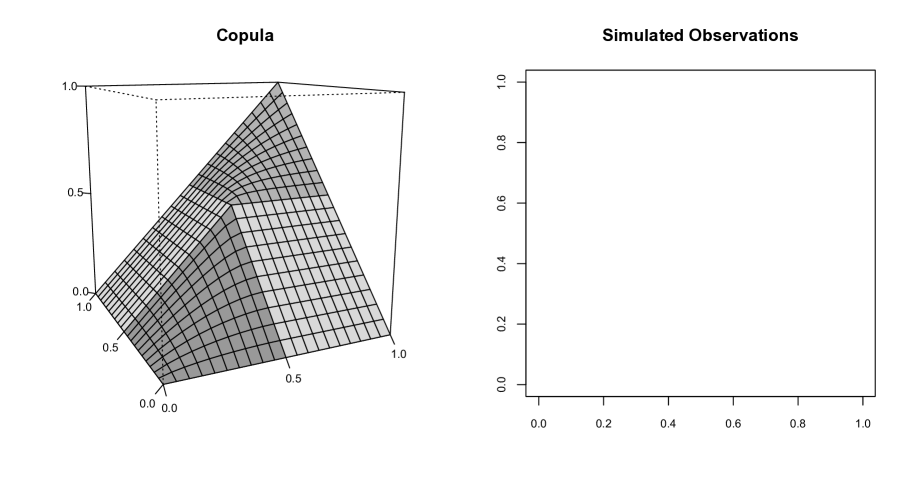
Figure 1: Left picture: Ordinal sum copula. Right picture: $500$ corresponding simulated observations.

In order to check for $C(q,q)=q$ for some $q\in(0,1)$ we propose the following modification of the statistic $\mathbb{T}_{n,\operatorname{M}}$

$$\mathbb{S}_{n,\operatorname{M}}=\mathbb{T}_{n,\operatorname{M}}+k_{n}\phi(A_{n}(C_{n})),$$

where $\mathbb{T}_{n,\operatorname{M}}$ is defined in (2.4) and (2.5), $k_{n}\sim n^{\alpha},\alpha\in(0,1/2)$ is some constant chosen by the statistician, $\phi$ is some increasing function with $\phi(0)=0$ and

$$A_{n}(C_{n})=\max\left\{\frac{i}{n}\left(1-\frac{i}{n}\right)\,:\,C_{n}\left(\frac{i}{n},\frac{i}{n}\right)=\frac{i}{n}\right\}.$$

Intuitively, $A_{n}(C_{n})$ should be “large” for copulas which satisfy $C(q,q)=q$ for some $q\in(0,1)$. For a decent choice of $k_{n}$ and $\phi$ we refer the reader to Section 4.

In Figure 2 we illustrate the points $i/n$ at which $C_{n}(i/n,i/n)=i/n$ for two specific examples, the Clayton copula with $\theta=1$ and the ordinal sum copula depicted in Figure 1. The solid and dashed lines correspond to the true copula and the empirical copula calculated for a set of $n=100$ observations, respectively. For the ordinal sum copula there always exist some points $i/n$ in a neighbourhood of $1/2$ such that $C_{n}(i/n,i/n)=i/n$, see the proof of the following Proposition, which is sufficient for the derivation of the asymptotic properties of the statistic $\mathbb{S}_{n,\operatorname{M}}$.

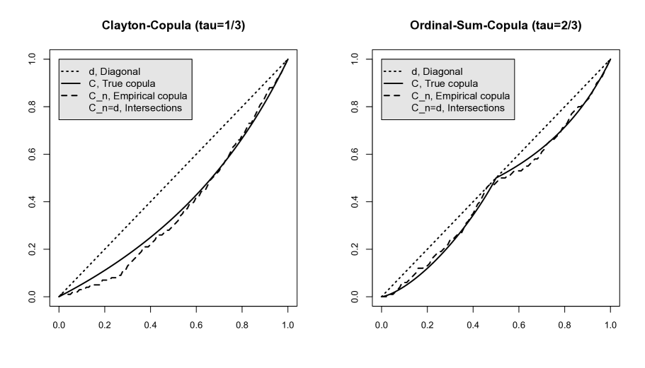
Figure 2: The solid lines show the diagonal section of a Clayton copula (left) and an ordinal sum copula (right), while the dashed line show one realization of the corresponding empirical copula. The circled points mark the locations where $C_{n}(i/n,i/n)=i/n$.

Proposition 3.1.

1. Suppose $C$ is an Archimedean copula satisfying Condition 2.1 and that the coefficients of tail dependence

   $$\lambda_{L}=\lim_{u\rightarrow 0}\frac{C(u,u)}{u}\quad\text{ and }\quad\lambda_{U}=\lim_{u\to 1}\frac{1-2u+C(u,u)}{1-u}$$

   exist and are smaller than $1$. Then it holds

   $$A_{n}(C_{n})=o_{\mathbb{P}}(n^{-\alpha})$$

   for any $\alpha<1/2$.

2. If there exists a $q\in(0,1)$ such that $C(q,q)=q$ then it holds

   $$A_{n}(C_{n})\geq q(1-q)+o_{\mathbb{P}}(1).$$

Proof. We start with the proof of a). First choose $\delta>0$ and $\lambda<1$ such that

$$\frac{C(u,u)}{u}\vee\frac{1-2u+C(u,u)}{1-u}\leq\lambda$$

for all $u\in[0,\delta]\cup[1-\delta,1]$ and use the decomposition

$$A_{n}(C_{n})=A_{n}(C_{n},[0,\delta))+A_{n}(C_{n},[\delta,1-\delta])+A_{n}(C_{n},(1-\delta,1]),$$ (3.1)

where

$$A_{n}(C_{n},B)=\max\left\{i/n\left(1-i/n\right)\,:\,C_{n}\left(i/n,i/n\right)=i/n\text{ and }i/n\in B\right\}$$

for some set $B\subset[0,1]$ (with the convention that $\max\emptyset=0$). Consider each term separately and define $M_{n}=\sup_{u\in[0,1]}\left|C_{n}(u,u)-C(u,u)\right|,$ which is of order $O_{\mathbb{P}}(n^{-1/2})$ under Condition 2.1. Now let $i/n\in(0,\delta)$ be such that $C_{n}(i/n,i/n)=i/n$. Due to the estimate

$$i/n(1-\lambda)\leq i/n\left(1-\frac{C(i/n,i/n)}{i/n}\right)=i/n-C(i/n,i/n)=C_{n}(i/n,i/n)-C(i/n,i/n)\leq M_{n}$$

we have $i/n(1-i/n)\leq i/n\leq M_{n}/(1-\lambda)$ and we can conclude that

$$A_{n}(C_{n},[0,\delta))\leq\frac{M_{n}}{1-\lambda}=O_{\mathbb{P}}(n^{-1/2}).$$ (3.2)

A similar calculation shows that for $i/n\in(1-\delta,1]$ with $C_{n}(i/n,i/n)=i/n$ we have $(1-i/n)(1-\lambda)\leq M_{n}$ which in turn implies

$$A_{n}(C_{n},(1-\delta,1])\leq\frac{M_{n}}{1-\lambda}=O_{\mathbb{P}}(n^{-1/2}).$$ (3.3)

It remains to estimate the second summand $A_{n}(C_{n},[\delta,1-\delta])$ of the decomposition (3.1). For continuity reasons we can choose a $\kappa>0$ such that $u-C(u,u)\geq\kappa$ for all $u\in[\delta,1-\delta]$. If there was a $q\in[\delta,1-\delta]$ such that $C_{n}(q,q)=q$, it would follow that $M_{n}\geq C_{n}(q,q)-C(q,q)\geq\kappa$ and therefore we have for any $\varepsilon>0$

$$\mathbb{P}\left(n^{\alpha}A_{n}(C_{n},[\delta,1-\delta]\right)>\varepsilon)\leq\mathbb{P}(\exists\,q\in[\delta,1-\delta]:C_{n}(q,q)=q)\leq\mathbb{P}(M_{n}\geq\kappa)\stackrel{{\scriptstyle\mathbb{P}}}{{\rightarrow}}0.$$

A combination of (3.2) and (3.3) with this result proves part a) of the proposition.

For the proof of part b) let $n_{1}=\#\{1\leq i\leq n:(F_{1}(X_{i1}),F_{2}(X_{i2}))\in[0,q]^{2}\}$. Since $C(q,q)=q$ implies that the mass of $C$ is concentrated on $(0,q)^{2}\cup(q,1)^{2}$ we have $(F_{1}(X_{i1}),F_{2}(X_{i2}))\in[0,q]^{2}$ if and only if $X_{i1}\leq X_{n_{1}:n,1}$ and $X_{i2}\leq X_{n_{1}:n,2}$, where $X_{j:n,p}=F_{np}^{-}(j/n)$ denotes the $j$-th order statistic of $X_{1p},\dots,X_{np}$ (for $p=1,2$). This yields $C_{n}(n_{1}/n,n_{1}/n)=n_{1}/n$, which entails the assertion by

$$A_{n}(C_{n})\geq\frac{n_{1}}{n}\left(1-\frac{n_{1}}{n}\right)\stackrel{{\scriptstyle\mathbb{P}}}{{\rightarrow}}q(1-q)>0.$$

∎

Remark 3.2.

1. The conditions on the coefficients of tail dependence in part a) of Proposition 3.1 can be equivalently expressed by conditions on the regular variation of the Archimedean generator of $C$. For a thorough discussion of these issues the reader is referred to the work of Charpentier and Segers, (2009).

2. Exploiting Theorem G.1 in Genest and Segers, (2009) and Proposition 4.2 in Segers, (2011) one can improve the rate of convergence in part a) of Proposition 3.1 to any $\alpha<3/4$. It is our conjecture that the term is in fact of order $O_{\mathbb{P}}(1/n)$, but we were not able to derive the asymptotic distribution of $nA_{n}(C_{n})$. Since we do not need a refined rate for our purposes here we omit a deeper discussion and defer these issues to future research.

From now on, suppose that the conditions of Theorem 2.3 and Proposition 3.1 hold. We can conclude that $\mathbb{S}_{n,\operatorname{M}}$ weakly converges to $\mathbb{T}_{C,\operatorname{M}}$ if the copula $C$ is Archimedean, while $\mathbb{S}_{n,\operatorname{M}}$ converges to $+\infty$ in probability if $C$ is non-Archimedean, i.e. if it is either non-associative (by the results of Section 2) or if there exists a $q\in(0,1)$ such that $C(q,q)=q$ (by Proposition 3.1). The quantiles of $\mathbb{T}_{C,\operatorname{M}}$ can be approximated by the multiplier method described in Section 2.2. Analogously to the discussion at the end of the Section 2.2 we can use the multiplier bootstrap to obtain an asymptotic level-$\alpha$ test for the hypothesis of Archimedeanity, which is consistent against all alternatives satisfying the Condition 2.1. Its finite sample properties will be investigated in the following section.

4 Finite sample properties

We conclude this paper with a simulation study regarding the finite sample performance of the proposed tests for Archimedeanity and Associativity. We consider the following six copula models:

• The Gumbel copula, which is Archimedean.

• The Clayton copula, which is Archimedean.

• The $t$-copula with fixed degree of freedom $df=1$, which is non-associative.

• The asymmetric negative logistic model [see Joe, (1990)] with fixed parameters $\psi_{1}=2/3,\psi_{2}=1$, which is non-associative.

• An ordinal sum model based on the partition $J_{1}=[0,1/2],J_{2}=[1/2,1]$ and the Gumbel $(C_{1})$ and Clayton $(C_{2})$ copula, denoted by $\text{Ordinal}_{A}$. The model is associative.

• An ordinal sum model based on the partition $J_{1}=[0,1/2],J_{2}=[1/2,1]$ and the two Clayton $(C_{1}=C_{2})$ copulas, denoted by $\text{Ordinal}_{B}$. The model is associative.

The parameters of the models are chosen in such a way that the coefficient of upper tail dependence $\lambda_{U}$ is either $1/4$ or $1/2$ [for the asymmetric negative logistic model] or that Kendall’s-$\tau$ is either $1/3$ or $2/3$ [for the remaining five models]. For $\tau_{\text{Ordinal}_{A}}=1/3$ (or $2/3$, resp.) we chose $\tau_{\text{Gumbel}}=0$ ($1/3$) and $\tau_{\text{Clayton}}=-2/3$ ($1/3$), while $\tau_{\text{Clayton}}=-1/3$ ($1/3$) for $\tau_{\text{Ordinal}_{B}}=1/3$ ($2/3$).

We generated $1000$ random samples of sample sizes $n=200$ and $n=500$ and calculated the empirical probability of rejecting the null hypotheses of Archimedeanity or Associativity for $\operatorname{M}\in\{\operatorname{L}^{2},\operatorname{KS}\}$. For each sample of size $n=200,500$ we carried out $B=200$ Bootstrap replications based on the multiplier method, where we chose a $\mathcal{U}(\{0,2\})$-distribution for the multipliers [i.e. $\mathbb{P}(\xi=0)=\mathbb{P}(\xi=2)=1/2$, s.t. $\mu=\tau=1$] and used $h=n^{-1/4}$ to estimate the partial derivatives. The critical values of the tests are determined by the method described in Section 2. The penalty term $\mathbb{S}_{n,\operatorname{M}}-\mathbb{T}_{n,\operatorname{M}}=k_{n}\phi(A_{n}(C_{n}))$ is chosen in the following data-adaptive way: first of all, we set $\phi(x)=(4x)^{2}$ in order to give more emphasis to values around the maximal value of $A_{n}(C_{n})$ [which equals $1/4$]. The constant $k_{n}$ is chosen according to the distribution of the bootstrap approximation: if $q^{\xi}_{0.05,\operatorname{M}}$ denotes the $0.05$-quantile of the sample $\{\mathbb{T}_{n,\operatorname{M}}^{\xi,b}\}_{b=1,\dots,B}$ we set $k_{n}=q^{\xi}_{0.05,\operatorname{M}}n^{1/4}$. The latter choice guarantees that under $H_{0}$ the error term is small compared to the distribution of $\mathbb{T}_{C,\operatorname{M}}$.

The results are stated in Table 1. The entries of the table represent the empirical probabilities of rejecting the null hypothesis of Archimedeanity and of Associativity [in brackets] for both the $\operatorname{L}^{2}$-test [first two columns] and the $\operatorname{KS}$-test [last two columns]. We observe that the nominal level of the four tests are accurately approximated for the four Archimedean copulas under investigation. The $\operatorname{L}^{2}$-test tends to be more conservative than the $\operatorname{KS}$-test. Also note that the values for $\mathbb{S}_{n,\operatorname{M}}$ and $\mathbb{T}_{n,\operatorname{M}}$ differ only by a very small amount meaning that the penalty term $k_{n}\phi(A_{n}(C_{n}))$ is of negligible magnitude under the null hypothesis.

The $t$-copula and the asymmetric negative logistic models are non-associative and the results in Table 1 reveal that these deviations are detected by both tests for Associativity, with better results for the $t$-copula and for stronger dependence [measured by either $\tau$ or $\lambda_{U}$]. The power properties of the $\operatorname{L}^{2}$-test outclass the properties of the $\operatorname{KS}$-test for all four non-associative models under investigation, such that the former test seems to be generally preferable.

Regarding the (associative) ordinal sum models both tests for associativity are very conservative. Note that the asymptotic theory developed in Section 2 does not apply for these models since the partial derivatives of the corresponding copulas are not continuous on $\{1/2\}\times[0,1]$ and $[0,1]\times\{1/2\}$. Regarding the power properties the $\operatorname{KS}$-test for Archimedeanity performs slightly better for the ordinal sum alternatives.

	$\operatorname{L}2$-Test			$\operatorname{KS}$-Test
	0.1	0.05		0.1	0.05
n=200:
Clayton($\tau=1/3$)	0.071 (0.071)	0.038 (0.037)		0.088 (0.088)	0.050 (0.050)
Clayton($\tau=2/3$)	0.030 (0.016)	0.011 (0.009)		0.124 (0.078)	0.068 (0.036)
Gumbel($\tau=1/3$)	0.079 (0.079)	0.043 (0.043)		0.082 (0.082)	0.046 (0.045)
Gumbel($\tau=2/3$)	0.034 (0.032)	0.015 (0.013)		0.108 (0.098)	0.065 (0.057)
$t(\tau=1/3,df=1)$	0.953 (0.953)	0.886 (0.884)		0.562 (0.558)	0.380 (0.376)
$t(\tau=2/3,df=1)$	0.748 (0.726)	0.592 (0.564)		0.392 (0.355)	0.258 (0.231)
Aneglog($\lambda_{U}=0.25$)	0.112 (0.112)	0.061 (0.061)		0.105 (0.105)	0.059 (0.059)
Aneglog($\lambda_{U}=0.5$)	0.641 (0.641)	0.536 (0.536)		0.363 (0.356)	0.225 (0.222)
$\text{Ordinal}_{A}(\tau=1/3)$	0.996 (0.000)	0.827 (0.000)		1.000 (0.012)	1.000 (0.005)
$\text{Ordinal}_{A}(\tau=2/3)$	1.000 (0.004)	1.000 (0.001)		1.000 (0.079)	1.000 (0.041)
$\text{Ordinal}_{B}(\tau=1/3)$	1.000 (0.000)	1.000 (0.000)		1.000 (0.045)	1.000 (0.021)
$\text{Ordinal}_{B}(\tau=2/3)$	1.000 (0.006)	1.000 (0.001)		1.000 (0.057)	1.000 (0.030)
n=500:
Clayton($\tau=1/3$)	0.082 (0.082)	0.051 (0.051)		0.088 (0.088)	0.036 (0.036)
Clayton($\tau=2/3$)	0.062 (0.059)	0.032 (0.027)		0.090 (0.082)	0.046 (0.039)
Gumbel($\tau=1/3$)	0.091 (0.091)	0.045 (0.045)		0.105 (0.105)	0.050 (0.050)
Gumbel($\tau=2/3$)	0.072 (0.070)	0.033 (0.032)		0.124 (0.121)	0.068 (0.066)
$t(\tau=1/3,df=1)$	1.000 (1.000)	1.000 (1.000)		0.954 (0.953)	0.871 (0.871)
$t(\tau=2/3,df=1)$	0.998 (0.990)	0.998 (0.990)		0.818 (0.811)	0.655 (0.650)
Aneglog($\lambda_{U}=0.25$)	0.237 (0.237)	0.173 (0.173)		0.124 (0.124)	0.069 (0.069)
Aneglog($\lambda_{U}=0.5$)	0.979 (0.979)	0.947 (0.947)		0.716 (0.716)	0.584 (0.584)
$\text{Ordinal}_{A}(\tau=1/3)$	1.000 (0.000)	0.980 (0.000)		1.000 (0.022)	1.000 (0.007)
$\text{Ordinal}_{A}(\tau=2/3)$	1.000 (0.021)	1.000 (0.009)		1.000 (0.093)	1.000 (0.038)
$\text{Ordinal}_{B}(\tau=1/3)$	1.000 (0.000)	1.000 (0.000)		1.000 (0.005)	1.000 (0.023)
$\text{Ordinal}_{B}(\tau=2/3)$	1.000 (0.013)	1.000 (0.004)		1.000 (0.082)	1.000 (0.037)

Table 1: Simulated rejection probabilities for the multiplier bootstrap-tests for Archimedeanity and for Associativity (in brackets). The sample size is $n=200$ or $n=500$, $B=200$ Bootstrap-replicates and 1000 simulation runs have been performed. The first four lines are Archimedean copula models, the $t$-models are not associative and the ordinal sum-models are associative, but not Archimedean.

Acknowledgements This work has been supported by the Collaborative Research Center “Statistical modeling of nonlinear dynamic processes” (SFB 823, Teilprojekt A1, C1) of the German Research Foundation (DFG).

References

- Alsina et al., (2006) Alsina, C., Frank, M. J., and Schweizer, B. (2006). Associative functions. World Scientific Publishing Co. Pte. Ltd., Hackensack, NJ. Triangular norms and copulas.
- Bücher, (2011) Bücher, A. (2011). Statistical inference for copulas and extremes. PhD thesis, Ruhr-University Bochum, Germany.
- Bücher and Dette, (2010) Bücher, A. and Dette, H. (2010). A note on bootstrap approximations for the empirical copula process. Statist. Probab. Lett., 80:1925–1932.
- Charpentier and Segers, (2009) Charpentier, A. and Segers, J. (2009). Tails of multivariate Archimedean copulas. J. Multivariate Anal., 100(7):1521–1537.
- Fermanian et al., (2004) Fermanian, J.-D., Radulović, D., and Wegkamp, M. (2004). Weak convergence of empirical copula processes. Bernoulli, 10(5):847–860.
- Genest and MacKay, (1986) Genest, C. and MacKay, R. J. (1986). Copules archimédiennes et familles de lois bidimensionnelles dont les marges sont données. Canad. J. Statist., 14(2):145–159.
- Genest et al., (2011) Genest, C., Nešlehová, J., and Ziegel, J. (2011). Inference in multivariate archimedean copula models. Test. to appear.
- Genest and Rivest, (1993) Genest, C. and Rivest, L.-P. (1993). Statistical inference procedures for bivariate Archimedean copulas. J. Amer. Statist. Assoc., 88(423):1034–1043.
- Genest and Segers, (2009) Genest, C. and Segers, J. (2009). Rank-based inference for bivariate extreme-value copulas. Ann. Statist., 37(5B):2990–3022.
- Jaworski, (2010) Jaworski, P. (2010). Testing archimedeanity. In Borgelt, C., González-Rodríguez, G., Trutschnig, W., Lubiano, M., Gil, M., Grzegorzewski, P., and Hryniewicz, O., editors, Combining Soft Computing and Statistical Methods in Data Analysis, volume 77 of Advances in Intelligent and Soft Computing, pages 353–360. Springer, Berlin.
- Joe, (1990) Joe, H. (1990). Families of min-stable multivariate exponential and multivariate extreme value distributions. Statist. Probab. Lett., 9(1):75–81.
- Kosorok, (2008) Kosorok, M. R. (2008). Introduction to Empirical Processes and Semiparametric Inference. Springer, New York.
- Ling, (1965) Ling, C.-h. (1965). Representation of associative functions. Publ. Math. Debrecen, 12:189–212.
- McNeil and Nešlehová, (2009) McNeil, A. J. and Nešlehová, J. (2009). Multivariate Archimedean copulas, -monotone functions and -norm symmetric distributions. Ann. Statist., 37(5B):3059–3097.
- Naifar, (2011) Naifar, N. (2011). Modelling dependence structure with Archimedean copulas and applications to the iTraxx CDS index. Journal of Computational and Applied Mathematics, 235:2459–2466.
- Nelsen, (2006) Nelsen, R. B. (2006). An introduction to copulas. Springer Series in Statistics. Springer, New York, second edition.
- Rémillard and Scaillet, (2009) Rémillard, B. and Scaillet, O. (2009). Testing for equality between two copulas. Journal of Multivariate Analysis, 100:377–386.
- Rivest and Wells, (2001) Rivest, L.-P. and Wells (2001). A martingale approach to the copula-graphic estimator for the survival function under dependent censoring. Journal of Multivariate Analysis, 79:138–.
- Rüschendorf, (1976) Rüschendorf, L. (1976). Asymptotic distributions of multivariate rank order statistics. Annals of Statistics, 4:912–923.
- Scaillet, (2005) Scaillet, O. (2005). A Kolmogorov-Smirnov type test for positive quadrant dependence. Canad. J. Statist., 33(3):415–427.
- Segers, (2010) Segers, J. (2010). Weak convergence of empirical copula processes under nonrestrictive smoothness assumptions. arXiv:1012.2133v1.
- Segers, (2011) Segers, J. (2011). Asymptotics of empirical copula processes under nonrestrictive smoothness assumptions. arXiv:1012.2133v2.
- Sklar, (1959) Sklar, A. (1959). Fonctions de répartition à dimensions et leurs marges. Publ. Inst. Statist. Univ. Paris, 8:229–231.
- Tsukahara, (2005) Tsukahara, H. (2005). Semiparametric estimation in copula models. Canad. J. Statist., 33(3):357–375.
- Van der Vaart and Wellner, (1996) Van der Vaart, A. W. and Wellner, J. A. (1996). Weak Convergence and Empirical Processes - Springer Series in Statistics. Springer, New York.
- Wang and Wells, (2000) Wang, W. and Wells, M. T. (2000). Model selection and semiparametric inference for bivariate failure-time data. Journal of the American Statistical Association, 95(449):62–72.