Testing the Low-Mass End of X-Ray Scaling Relations
with a Sample of Chandra Galaxy Groups

Abstract

Context. Well-determined scaling relations between X-ray observables and cluster mass are essential for using large cluster samples to constrain fundamental cosmological parameters. Scaling relations between cluster masses and observables, such as the luminosity-temperature, mass-temperature, luminosity-mass relations, have been investigated extensively, however the question of whether these relations hold true also for poor clusters and groups remains unsettled. Some evidence supports a “break” at the low end of the group/cluster mass range, possibly caused by the stronger influence of non-gravitational physics on low-mass systems.

Aims. The main goal of this work is to test local scaling relations for the low-mass range in order to check whether or not there is a systematic difference between clusters and groups, and to thereby extend this method of reliable and convenient cluster mass determination for future large samples down to the group regime.

Methods. We compiled a statistically complete sample of 112 X-ray galaxy groups, 26 of which have usable Chandra data. Temperature, metallicity, and surface brightness profiles were created for these 26 groups, and used to determine the main physical quantities and scaling relations. We then compared the group properties to those of the HIFLUGCS clusters, as well as several other group and cluster samples.

Results. We present radial profiles for the individual objects and scaling relations of the whole sample ($L_{\text{x}}$-$T$, $M$-$T$, $L_{\text{x}}$-$M$, $M_{\text{g}}$-$M$, $M$-$Y_{\text{x}}$, $L_{\text{x}}$-$Y_{\text{x}}$, $f_{\text{g}}$-$T$). Temperature and metallicity profiles behave universally, except for the core regions. The $L_{\text{x}}$-$T$, $M$-$T$, $L_{\text{x}}$-$M$, $M_{\text{g}}$-$M$, $M$-$Y_{\text{x}}$, and $L_{\text{x}}$-$Y_{\text{x}}$ relations of the group sample are generally in good agreement with clusters. The $L_{\text{x}}$-$T$ relation steepens for $T<3\,\mathrm{keV}$, which could point to a larger impact of heating mechanisms on cooler systems. We found a significant drop in the gas mass fraction below $\lesssim 1\,\mathrm{keV}$, as well as a correlation with radius, which indicates the ICM is less dominant in groups compared to clusters and the galaxies have a stronger influence on the global properties of the system. In all relations the intrinsic scatter for groups is larger than for clusters, which appears not to be correlated with merger activity but could be due to scatter caused by baryonic physics in the group cores. We also demonstrate the importance of selection effects.

Conclusions. We have found some evidence for a similarity break between groups and clusters. However this does not have a strong effect on the scaling relations.

1 Introduction

Clusters of galaxies are excellent tools for measuring fundamental cosmological parameters such as the mean matter density $\Omega_{\text{m}}$ and the amplitude of primordial density fluctuations, $\sigma_{8}$. These can readily be constrained by comparing theoretical predictions to the observed cluster mass function, but only if the masses are well-determined and not affected by systematic bias.

X-ray emission from the intracluster medium (ICM) provides one of the main instruments to measure the mass, as well as a wide range of additional physical gas properties, e. g. temperature, metallicity, gas density, entropy, luminosity, and also to investigate the dynamical state. However, for samples of hundreds of objects and future surveys encompassing up to $100,000$ clusters, like eROSITA (e. g. Predehl et al. 2010), it is convenient and essential to use reliable mass-observable relations instead of determining masses individually for each cluster.

The total gravitational mass of a cluster, consisting of both baryonic matter and dark matter, is tightly correlated with observable quantities such as temperature and luminosity, and relations between these have been studied extensively with both observational and computational techniques (e. g. Allen et al. 2001, Finoguenov et al. 2001, Reiprich & Böhringer 2002, Borgani et al. 2004, Stanek et al. 2006, Nagai et al. 2007, Rykoff et al. 2008, Hartley et al. 2008, Zhang et al. 2008, Lopes et al. 2009, Vikhlinin et al. 2009, Ettori et al. 2010, Leauthaud et al. 2010, Mantz et al. 2010, Plagge et al. 2010).

Groups and poor clusters of galaxies are more common than rich clusters due to the steepness of the cluster mass function, and they contain a total amount of hot gas comparable to or even larger than that of all rich clusters combined. However, at the same time they are fainter and cooler, and thus generally more difficult to detect and distinguish from the background, especially at higher redshifts. So only recently, with the advent of highly sensitive, high-resolution X-ray observatories like Chandra and XMM-Newton, have groups been studied to a greater extent. Over the last decade, many independent investigations have found indications that groups cannot simply be treated as less massive, “scaled-down” cluster specimen, but must be considered as a unique class of objects, for a number of reasons.

First of all, groups are different from clusters simply in that they are cooler, less massive systems with shallower potential wells. But because of this they are also expected to be more strongly affected by non-gravitational mechanisms such as galactic winds or feedback from supernovae, cosmic rays, and active galactic nuclei (AGN). These influences are complex and difficult to reproduce in simulations, and thus require careful cross-checking with observations. These processes are suspected of systematically increasing intrinsic scatter and changing global properties of groups.

Also, the matter composition in groups is different from that in clusters. While in clusters the ICM strongly dominates over the galactic component, in groups the situation is turned around, and the combined mass of the member galaxies may even exceed that of the gas (e. g. Giodini et al. 2009). Accordingly, e. g. Dell’Antonio et al. (1994) and Mulchaey & Zabludoff (1998) suggested that two distinct X-ray emitting components coexist in groups, which have to be considered separately, one of which is extended and consists of hot diffuse gas bound to the group potential, and a second component, which is associated with the halos of member galaxies. Jeltema et al. (2008a) also showed that the member galaxies have a higher chance of retaining their gas halos in group environments because these have lower densities and gas stripping is not nearly as efficient as it is in clusters.

In terms of mass and richness, groups naturally stand as an intermediate class between isolated field galaxies on one hand and rich clusters, typically containing thousands of galaxies, on the other. In groups the average galaxy velocity dispersions are much lower than in clusters, close to the relative velocities of single galaxies, increasing the probability of galaxy-galaxy interactions and mergers, making groups the most attractive environments to study these activities.

As the physical emission processes in the ICM are strongly dependent on the gas temperature, the X-ray emission spectra from low-temperature groups are typically dominated by line emission, not bremsstrahlung continuum emission which is dominant in hotter objects with $T\gtrsim 2\,\mathrm{keV}$.

Many investigations have found or predicted a systematic difference between the physical properties of groups compared to clusters, e. g. a flatter $L_{x}$-$\sigma$ relation (Mahdavi et al. 2000, Xue & Wu 2000b), or a steepening of the $L_{x}$-$T$ relation (e. g. Ponman et al. 1996, Xue & Wu 2000b, Helsdon & Ponman 2000, Davé et al. 2008). Pope (2009) predicted analytically that AGN feedback should not affect the $L_{x}$-$\sigma$ relation above $\sigma\sim 500\,\mathrm{km\leavevmode\nobreak\ s^{-1}}$, corresponding to temperatures around $1-2\,\mathrm{keV}$, which could explain a similarity break in the $L_{x}$-$T$ relation. Sanderson et al. (2003) found a break and gradual steepening in the $M$-$T$ relation measured over a wide range of objects, spanning from elliptical galaxies to clusters. Finoguenov et al. (2001) also reported a steeper $M$-$T$ slope than the cluster relation when groups are included in the fit. Maughan et al. (2011) found an observed steepening of the $L_{x}$-$T$ relation of relaxed clusters below $3.5\,\mathrm{keV}$ and argue it is caused by central heating that affects the ICM out to a larger radius in lower mass systems. This would also be in agreement with the findings of Mittal et al. (2011), who suggested that for systems below $2.5\,\mathrm{keV}$ AGN heating becomes a more important influence on the $L_{x}$-$T$ relation than ICM cooling, which is dominant in hotter clusters.

On the other hand, a number of studies do not support the discrepancy between groups and clusters, but instead get consistent results for the whole observed mass range, albeit often with larger scatter for groups, as for the $L_{\text{x}}$-$\sigma$, $L_{\text{x}}$-$T$, $M$-$T$, $\sigma$-$T$, $M$-$T$, and $M$-$Y_{\text{x}}$ relations (e. g. Mulchaey & Zabludoff 1998, Osmond & Ponman 2004, Sun et al. 2009).

Khosroshahi et al. (2007) investigated fossil groups in particular and found that fossils are hotter and brighter for a given mass than non-fossil groups, suggesting they follow more closely an extension of cluster properties. Similarly, Balogh et al. (2010) found a dichotomy in the X-ray gas properties of low-mass clusters and groups selected by $\sigma$. This might explain why observations of groups seem to yield larger scatter and inconsistent results, namely there could be different types of groups involved. Intracluster magnetic fields may also affect the scaling relations more strongly for the low-temperature range, resulting in an effective steepening, as proposed by Colafrancesco & Giordano (2007).

Another hint for a possible change in the properties of groups is the mass fraction $f_{\text{g}}$ of the hot gas component compared to the total mass. This parameter remains quite constant over the cluster regime, yet e. g. Reiprich (2001), Gastaldello et al. (2007), and Dai et al. (2010) detected a decrease in $f_{\text{g}}$ towards the low-mass, low-temperature end. Croston et al. (2008) and Pratt et al. (2009) suggest that a dependence of $f_{\text{g}}$ on temperature and mass may be responsible for the steepening in scaling relations. Sun et al. (2009) find a lower gas fraction as well, but only for the region within a small fiducial radius, so they argue the global $f_{\text{g}}$ in groups may be decreased by lower gas fractions within the central region alone. This would be in agreement with the findings of Zhang et al. (2010), who detect a correlation of gas fraction and cluster radius. However Sanderson et al. (2003) report a systematic trend in $f_{\text{g}}$ with temperature in all but the central regions.

The main goal of this work is to investigate whether or not there is a “break” by testing the main cluster scaling relations for a sample of galaxy groups. We used essentially the same reduction and analysis pipelines that were applied to the HIFLUGCS clusters (Hudson et al. 2010), so the results of both samples are directly comparable. We investigated the $L_{\text{x}}$-$T$, $M$-$T$, $L_{\text{x}}$-$M$, $M_{\text{g}}$-$M$, $M$-$Y_{\text{x}}$, $L_{\text{x}}$-$Y_{\text{x}}$, and $f_{\text{g}}$-$T$ relations, for both $r_{2500}$ and $r_{500}$, where $Y_{\text{x}}$ is defined as the product of temperature and gas mass, which has been introduced in order to reduce scatter and bias from merger activity (Kravtsov et al. 2006), and where the $r_{\Delta}$ is defined as the radius within which the matter density is $\Delta$ times the critical density of the Universe and which encloses the total matter $M_{\Delta}$.

Merging events are problematic for cluster scaling relations because they have a large impact on the global properties of the system, strongly boosting luminosity and temperature via shock-heating for a certain time but also often biasing low the measured temperature due to unthermalized gas, cool clumps and substructure (e. g. Mathiesen & Evrard 2001, Ricker & Sarazin 2001, Ritchie & Thomas 2002, Hartley et al. 2008, Yang et al. 2009, Böhringer et al. 2010, Takizawa et al. 2010). Another issue is the fact that X-ray mass estimates must rely on the fundamental assumptions of hydrostatic equilibrium and spherical symmetry, which are expected to be broken in merging systems and may take several Gyr to re-establish (Ritchie & Thomas 2002). Tovmassian & Plionis (2009) even state that groups in general are not in equilibrium but still in the process of virialization.

Including only regular, relaxed systems could in principle reduce scatter and bias in scaling relations, but identifying mergers is not trivial, for instance in the most extreme case a merger along the line-of-sight will appear perfectly symmetric in the X-ray emission, so it may probably not be possible to reliably determine the true dynamical state going by the surface brightness distribution alone (Nagai et al. 2007a, Jeltema et al. 2008b, Ventimiglia et al. 2008, Riemer-Sørensen et al. 2009, Zhang et al. 2009). We did not exclude any irregular groups, and so did not bias our sample with respect to morphology. We do however investigate whether excluding unrelaxed objects changes the scaling relations significantly (see section 4.3).

However we took care in the global temperature fits to exclude the central region of groups with cooling cores that are strongly influenced by complex baryonic physics not yet fully understood, which, if not excluded, will introduce a large degree of scatter on the luminosity-temperature and luminosity-mass relations (Markevitch 1998, Loken et al. 2002, Sanderson et al. 2006, Chen et al. 2007, Mittal et al. 2009, Pratt et al. 2009, Hudson et al. 2010).

This paper is organized as follows. We begin with the selection of the group sample in section 2. In section 3 we outline the analysis methods. We present our results in section 4 and discuss and compare them to other work in section 5. A summary and our conclusions are given in section 6. Radial profiles, images and notes for individual objects are included in the appendix. Throughout this paper, we assume a flat $\Lambda$CDM cosmology with $\Omega_{\text{m}}=0.3$, $\Omega_{\Lambda}=0.7$, and $h=0.7$, where $H_{0}=100\,h\,\mathrm{km\,s^{-1}\,Mpc^{-1}}$ is the Hubble constant. X-ray luminosities $L_{\text{x}}$ and fluxes $f_{\text{x}}$ are given in the range of $0.1-2.4\,\mathrm{keV}$ (“ROSAT band”). Logarithms are decadic.

Figure 1: Left: X-ray fluxes of the 26 groups plotted against redshift. The dashed line is the HIFLUGCS limit. Right: X-ray luminosities plotted against redshift. The dashed line is the upper luminosity cut applied here. One object appears outside the limit due to conflicting luminosity measurements (section 2).

2 Sample Selection

The group sample presented in this work was compiled from the X-ray selected, highly complete HIFLUGCS, NORAS, and REFLEX catalogues (Reiprich & Böhringer 2002, Böhringer et al. 2000, and Böhringer et al. 2004, respectively). We selected groups by applying an upper limit to the X-ray luminosity $L_{\text{x}}$, which was determined homogeneously for all three parent catalogues, plus a lower redshift cut to exclude objects that are too close to be observed out to sufficiently large radii:

$$L_{\text{x}}<5\cdot 10^{43}\,h^{-2}_{50}\,\mathrm{erg\,s^{-1}}=2.55\cdot 10^{43}\,h^{-2}_{70}\,\mathrm{erg\,s^{-1}},\text{and }z>0.01.$$

This selection yields a statistically complete sample of 112 X-ray selected galaxy groups. In this work only those groups were investigated that have been observed with the Chandra telescope with sufficient exposure time ($\gtrsim 10\,\mathrm{ks}$). Of these 27 objects, listed in Table 1, one (IC4296) in the end had to be excluded from the scaling relations for technical reasons, but will still appear in some of the tables (for more details see section A in the appendix). We do not consider any redshift evolution for our scaling relations, as this is a local sample (median redshift $0.025$). The fluxes and luminosities of the remaining 26 groups are plotted against redshift in Fig. 1. The effect of flux limits applied to the parent samples appears as a deficiency of faint objects at high redshifts in the luminosity plot.

A few groups are included in more than one catalogue and thus have several luminosity measurements. For those objects present in the HIFLUGCS sample, we adopted this luminosity measurement, for the others we preferred the value obtained with REFLEX. In one case (MKW8) the measured values differ by $50\,\mathrm{\%}$ between HIFLUGCS and NORAS, where the former measurement places the group outside the luminosity cut. We however kept this object in the sample because the luminosity obtained with NORAS lies well within the cut.

As mentioned in the previous section, we avoided morphology bias by not performing any morphological selection, however the results of this work may be affected by “archival bias” as we so far have relied on what was available in the Chandra archives.

In future work we will continue to complete this sample, starting with observational data taken with XMM-Newton. For the full sample more observations will be necessary, since some of the groups on the selection list have not been observed with either XMM-Newton or Chandra.

Table 1: Properties of the group sample

Group Name	RA	DEC	$z$	$n_{\text{H}}$	$f_{\text{x}}$	$L_{\text{x}}$	$L_{\text{x}}$ error
	J2000	J2000		$10^{20}\,\mathrm{cm^{-2}}$	$10^{-12}\,\mathrm{erg\,s^{-1}\,cm^{-2}}$	$10^{44}\,h^{-2}_{70}\,\mathrm{erg\,s^{-1}}$	%
A0160	01 13 02.287	+15 29 46.37	0.0447	3.98	4.34	0.198	14.1
A1177	11 09 44.387	+21 45 42.25	0.0316	5.51*	3.74	0.090	14.3
ESO552020	04 54 50.639	-18 06 46.99	0.033456	4.45	5.54	0.142	11.8
HCG62	12 53 05.419	-09 12 17.54	0.0137	3.55	6.54	0.031	13.2
HCG97	23 47 23.672	-02 18 13.70	0.0218	14.82*	2.63	0.030	38.8
IC1262	17 33 01.027	+43 45 32.85	0.034394	3.27*	11.55	0.248	5.1
IC1633	01 09 54.500	-45 54 22.67	0.02425	1.91	14.01	0.179	8.0
IC4296	13 36 37.460	-33 58 37.99	0.012465	4.14	2.35	0.008	16.4
MKW4	12 04 26.365	+01 53 51.34	0.02	3.61*	22.68	0.203	1.7
MKW8	14 40 37.939	+03 27 50.15	0.027	2.34	25.25	0.414	8.4
NGC326	00 58 21.121	+26 52 57.91	0.047	17.30*	4.92	0.230	12.9
NGC507	01 23 38.670	+33 15 24.93	0.01902	5.56	21.12	0.129	1.3
NGC533	01 25 32.066	+01 45 22.28	0.017385	3.12	4.71	0.032	15.9
NGC777	02 00 14.235	+31 25 24.63	0.016728	4.72	3.36	0.021	14.0
NGC1132	02 52 50.838	-01 16 35.64	0.024213	5.56	6.03	0.075	16.2
NGC1550	04 19 37.695	+02 24 30.46	0.0123	13.35*	46.32	0.156	5.4
NGC4325	12 23 06.592	+10 37 13.26	0.0257	5.95*	7.01	0.105	7.8
NGC4936	13 04 16.392	-30 32 08.23	0.0117	6.49	8.28	0.025	13.6
NGC5129	13 24 09.943	+13 58 46.11	0.023176	11.04*	2.96	0.037	17.1
NGC5419	14 03 37.462	-33 59 09.24	0.014	5.16	8.08	0.032	14.4
NGC6269	16 57 58.730	+27 51 22.43	0.034424	6.80*	7.33	0.190	8.2
NGC6338	17 15 21.347	+57 24 43.94	0.028236	2.29	14.81	0.257	15.4
NGC6482	17 51 48.948	+23 04 21.76	0.013129	14.72*	2.84	0.010	10.9
RXCJ1022.0+3830	10 22 10.353	+38 31 25.57	0.0491	6.02*	3.37	0.188	28.3
RXCJ2214.8+1350	22 14 46.016	+13 50 50.80	0.0263	4.57	3.24	0.047	18.1
S0463	04 28 38.623	-53 50 46.01	0.0394	2.40*	4.02	0.148	16.5
SS2B153	10 50 26.346	-12 50 44.69	0.0154	10.16*	10.93	0.059	6.8

• Notes: Coordinates are given for the emission-weighted center. $L_{\text{x}}$ and $f_{\text{x}}$ are given in the $0.1-2.4\,\mathrm{keV}$ band. For REFLEX and NORAS objects we quote the corrected fluxes. Galactic $n_{\text{H}}$ values taken from the LAB survey, fitted values are marked with an asterisk.

3 Data Analysis

The observations used are listed in Table 6 in the appendix. In two cases, NGC507 and NGC1132, one of two available data sets was badly flared, so we completely excluded it and relied solely on the other one. For HCG62 there were four observations available, however of the first two, one was from an early epoch and the other had only $5\,\mathrm{ks}$, so we used the newer data sets, which combined add up to $120\,\mathrm{ks}$.

All data sets were reduced using CIAO $3.4$ with CALDB $3.3$, following the procedures given in the CIAO Science Threads and in M. Markevitch’s cookbook.

In general the data analysis was carried out in the same way as described in Hudson et al. (2006 and 2010), apart from minor modifications described below, so only a brief outline of the methods will be given here.

Background subtraction was done using the ACIS blank-sky background files, correcting for possible differences in the Galactic foreground emission between science and background observations.

The emission peak (EP) and emission-weighted center (EWC) for each group were determined from adaptively smoothed, background-subtracted, exposure-corrected images. In most cases the EP and the EWC coincide, though in groups with irregular morphology they can be separated by several arcminutes (Table 2). The temperature, metallicity, and surface brightness profiles were all centered on the EWC, which we consider more appropriate for studying the outer parts of the group and the overall morphology, while the EP was used only to estimate the core region to be excluded from the global temperature determination.

3.1 Global Temperature

The global temperatures and metallicities were determined by fitting the whole observed area to a single spectrum. The temperature may be strongly biased by a cooler gas component at the center, detectable as a central temperature drop. In order to minimize this bias, we investigated temperature profiles centered on the EP to determine how large a region should be excluded from the fit. The cutoff radii for individual objects are given in Table 2.

We slightly modified the core cutoff estimation method from the HIFLUGCS analysis (Hudson et al. 2010), as for the fainter systems in our sample there are relatively few source counts and radial bins. In cases where there were so few counts that the temperature profile consisted of only 5 or fewer bins, no central region was excluded at all. The other profiles were fit with a two-component function, consisting of a powerlaw for the central region and a constant beyond the cutoff radius, to account for the flat plateau found in typical profiles at intermediate radii. In cases where there were one or two bins at large radii significantly lower than the plateau, they were ignored in this fit, as they are the least important for the core region. The cutoff radius between central and flat region was varied iteratively, starting from the center, until the reduced $\chi^{2}$ of the combined fit reached a minimum. The outer radius of the annulus with the best fit statistic was then set as the cutoff radius. We did not simply use a fixed fraction of the virial radius as core estimate because there is evidence the cutoff radius does not scale uniformly with $r_{\text{vir}}$ (Hudson et al. 2010).

3.2 Temperature and Metallicity Profiles

For the radial temperature and metallicity profiles, successive annular regions were created around the EWC. We required that each ring contain the same number of source counts, $2500$, $5000$ or $10,000$, depending on the brightness of the object and the depth of the available data. The outermost annulli with fewer counts were still included in the profiles if the spectral fit reasonably constrained the temperature.

Temperature $T$ and metallicity $Z$ (relative to the solar abundances measured by Anders & Grevesse 1989) were fit simultaneously for each annulus, with the hydrogen column density $n_{\text{H}}$ fixed to the LAB value. In some cases we found the $n_{\text{H}}$ value to be significantly too low, so we left this parameter free in the fits (marked by an asterisk in Table 1).

In our fit models we use one apec component for the ICM, and another to account for possible over- or undersubtraction of the CXB, as estimated from the outer regions. In some cases we found it necessary to include an unfolded powerlaw component as well, to account for unresolved AGN emission or soft proton flares, especially in the BI chips (S1 and S3). In cases where the reduced $\chi^{2}\gtrsim 1.3$, slight model variations were used to improve the fit. In some cases we tried an apec model with separate abundances for the most common elements. We found the reduced $\chi^{2}$ could be improved slightly but the best fit parameters remained unchanged, so we chose to keep the regular model. For several objects, the fit to the innermost annuli was not very good, but could be significantly improved by fitting a second apec component, probably due to the presence of multi-temperature gas at the center.

For the mass calculation we also determined the temperature gradient by fitting a powerlaw function to the profile, excluding the same core region as for the global temperature (see above). We used a simple powerlaw function, which we found to describe the data reasonably well (see the plots in section C of the appendix):

$$\log\left(\frac{T}{T_{\text{mid}}}\right)=a\cdot\log\left(\frac{r}{r_{\text{mid}}}\right)+b,$$ (1)

where $\log r_{\text{mid}}=(\log r_{\text{min}}+\log r_{\text{max}})/2$ and $T_{\text{mid}}=(\log T_{\text{min}}+\log T_{\text{max}})/2$.

3.3 Surface Brightness Profiles

Surface brightness profiles (SBPs) were extracted from narrow annular regions in the energy range of $0.1-2.0\,\mathrm{keV}$, with $\sim 500$ source counts per radial bin. Each profile was fit with a double $\beta$-model (e. g. Cavaliere & Fusco-Femiano 1976), which is the superposition of two surface brightness components with respective core radii $x_{\text{ci}}$, $\beta$ parameters $\beta_{\text{i}}$, and central surface brightness $\Sigma_{0}=\Sigma_{01}+\Sigma_{02}$:

$$\Sigma(x)=\Sigma_{01}\left(1+\frac{x^{2}}{x_{\text{c1}}^{2}}\right)^{-3\beta_{1}+\frac{1}{2}}+\Sigma_{02}\left(1+\frac{x^{2}}{x_{\text{c2}}^{2}}\right)^{-3\beta_{2}+\frac{1}{2}},$$ (2)

and which yields the corresponding density profile

$$n(r)=\sqrt{n^{2}_{01}\left(1+\frac{r^{2}}{r_{\text{c1}}^{2}}\right)^{-3\beta_{1}}+n^{2}_{02}\left(1+\frac{r^{2}}{r_{\text{c2}}^{2}}\right)^{-3\beta_{2}}},$$ (3)

via these relations:

$$n^{2}_{01}=\frac{\Sigma_{12}LI_{2}}{\Sigma_{12}LI_{2}+LI_{1}}n^{2}_{0},\quad\text{and}\quad n^{2}_{02}=\frac{LI_{1}}{\Sigma_{12}LI_{2}+LI_{1}}n^{2}_{0}.$$ (4)

The central electron density, $n_{0}$, is given by

$$n_{0}=\left(\frac{10^{14}\leavevmode\nobreak\ 4\pi\leavevmode\nobreak\ (\Sigma_{12}\leavevmode\nobreak\ LI_{2}+LI_{1})\leavevmode\nobreak\ D_{\text{A}}\leavevmode\nobreak\ D_{\text{L}}\leavevmode\nobreak\ \zeta\leavevmode\nobreak\ n}{\Sigma_{12}\leavevmode\nobreak\ LI_{2}\leavevmode\nobreak\ EI_{1}+LI_{1}\leavevmode\nobreak\ EI_{2}}\right)^{1/2},$$ (5)

where $D_{\text{A}}$ and $D_{\text{L}}$ are the angular diameter and luminosity distances, respectively, $\zeta$ is the ratio of electrons to protons, $n$ is the normalization of the apec model, $EI_{\text{i}}$ is the emission integral for model i,

$$EI_{\text{i}}=2\pi\int\int^{R}_{0}x\leavevmode\nobreak\ \left(1+\frac{x^{2}+l^{2}}{x^{2}_{\text{ci}}}\right)^{-3\beta_{\text{i}}}\leavevmode\nobreak\ \text{d}x\leavevmode\nobreak\ \text{d}l,$$ (6)

and

$$LI_{\text{i}}=\int\left(1+\frac{z^{2}}{x_{\text{ci}}^{2}}\right)^{-3\beta_{\text{i}}}\text{d}z$$ (7)

is the line integral along the line of sight (for $i=[1,2]$) and $\Sigma_{12}$ is the ratio of $\Sigma_{01}$ and $\Sigma_{02}$. $x_{\text{ci}}$ is the projected length of $r_{\text{ci}}$.

In one case, NGC777, the data was only sufficient to fit a single $\beta$-model. Since the slope of the outer $\beta$ component has the greatest influence on the mass calculation, we put more weight on this component by fitting the outer part separately and fixing the slope in the overall fit. Some irregular or asymmetric groups have small humps close to the center, which are likely caused by an offset between the emission peak and the emission-weighted center, on which the SBPs are centered, or by a secondary peak, e. g. in a merging system. In a few cases we excluded these spikes when fitting the SBP, which improved the fit statistic but did not significantly change the final fit parameters of the $\beta$-model.

3.4 Mass Determination

The total mass within radius $r$ can be estimated assuming hydrostatic equilibrium and spherical symmetry, using the density gradient as well as the temperature gradient:

$$M(<r)=-\frac{1}{G}\frac{k_{\text{B}}Tr}{\mu m_{\text{p}}}\left(\frac{\text{d}\ln\rho_{\text{g}}}{\text{d}\ln r}+\frac{\text{d}\ln T}{\text{d}\ln r}\right),$$ (8)

where $G$ is the gravitational constant, $\mu$ is the gas mean molecular weight ($\mu\approx 0.6$), and $m_{\text{p}}$ is the proton mass. Plugging in eqns. (1) and (3) for the temperature and density gradients, we arrive at:

$$M(<r)=\frac{3r^{3}}{G}\frac{T(r)}{\mu m_{\text{p}}}\left(\frac{\Sigma_{12}LI_{2}\zeta^{\prime}_{1}+LI_{1}\zeta^{\prime}_{2}}{\Sigma_{12}LI_{2}\zeta_{1}+LI_{1}\zeta_{2}}-a\right),$$ (9)

where $a$ is the slope of the temperature profile (eqn. 1) and

$$\zeta_{\text{i}}=\left(1+\frac{r^{2}}{r_{\text{ci}}^{2}}\right)^{-\frac{3\beta_{\text{i}}}{2}}\quad\text{and}\quad\zeta^{\prime}_{\text{i}}=\frac{\beta_{\text{i}}}{r_{\text{ci}}^{2}}\left(1+\frac{r^{2}}{r_{\text{ci}}^{2}}\right)^{-\frac{3\beta_{\text{i}}}{2}-1}.$$ (10)

In the double $\beta$-model fits $r_{\text{c1}}$, $r_{\text{c2}}$, $\beta_{1}$ and $\beta_{2}$ are highly degenerate, resulting in unphysically large errors (often $\sim 100\,\mathrm{\%}$). For this reason we used a Monte Carlo simulation to estimate the uncertainties. With this we created 1000 temperature and surface brightness profiles varied according to the statistical errors and used the standard deviation of the mass values derived from each variation as an estimate of the statistical uncertainty on total mass and gas mass.

The gas mass within $r$ can be calculated using eqn. (3) and

$$M_{\text{g}}(<r)=\mu m_{\text{p}}\left(1+\frac{n_{\text{e}}}{n_{\text{p}}}\right)\int n(r)\,\text{d}V,$$ (11)

where $n_{\text{e}}$ and $n_{\text{p}}$ are the electron and proton number densities.

The fiducial radii $r_{2500}$ and $r_{500}$ were determined iteratively by integration of the total mass profiles.

3.5 Scaling Relations

Linear regressions for the scaling relations were calculated in log-log space, using the bisector statistic of the BCES_REGRESS code (Akritas & Bershady 1996), which takes into account the uncertainties on both the $X$ and $Y$ parameters. The errors were estimated with $10\,000$ bootstrapping iterations. We used the following functions for fitting:

$$\log\left(\frac{L_{\text{x}}}{0.5\cdot 10^{44}\,h^{-2}_{70}\,\mathrm{erg\,s^{-1}}}\right) = a\cdot\log\left(\frac{T}{3\,\mathrm{keV}}\right)+b,$$ (12)

$$\log\left(\frac{M_{\text{r}}}{10^{14}\,h^{-1}_{70}\leavevmode\nobreak\ M_{\odot}\,\mathrm{}}\right) = a\cdot\log\left(\frac{T}{3\,\mathrm{keV}}\right)+b,$$ (13)

$$\log\left(\frac{L_{\text{x}}}{0.5\cdot 10^{44}\,h^{-2}_{70}\,\mathrm{erg\,s^{-1}}}\right) = a\cdot\log\left(\frac{M_{\text{r}}}{10^{14}\,h^{-1}_{70}\leavevmode\nobreak\ M_{\odot}\,\mathrm{}}\right)+b,$$ (14)

$$\log\left(\frac{M_{\text{r}}}{10^{14}\,h^{-1}_{70}\leavevmode\nobreak\ M_{\odot}\,\mathrm{}}\right) = a\cdot\log\left(\frac{Y_{\text{x}}}{10^{12}\,h^{-5/2}_{70}\leavevmode\nobreak\ M_{\odot}\,\mathrm{}}\right)+b,$$ (15)

$$\log\left(\frac{L_{\text{x}}}{0.5\cdot 10^{44}\,h^{-2}_{70}\,\mathrm{erg\,s^{-1}}}\right) = a\cdot\log\left(\frac{Y_{\text{x}}}{10^{12}\,h^{-5/2}_{70}\leavevmode\nobreak\ M_{\odot}\,\mathrm{}}\right)+b,$$ (16)

$$\log\left(\frac{M_{\text{g,r}}}{10^{12}\,h^{-5/2}_{70}\leavevmode\nobreak\ M_{\odot}\,\mathrm{}}\right) = a\cdot\log\left(\frac{M_{\text{r}}}{10^{14}\,h^{-1}_{70}\leavevmode\nobreak\ M_{\odot}\,\mathrm{}}\right)+b,$$ (17)

$$\log\left(\frac{f_{\text{g,r}}}{0.1\cdot h^{-3/2_{70}}}\right) = a\cdot\log\left(\frac{T}{3\,\mathrm{keV}}\right)+b,$$ (18)

where $r$ is $r_{2500}$ or $r_{500}$, respectively.

The total logarithmic scatter is given by $\sigma^{X}_{\text{tot}}=\langle(\log X-(\log Y-b)/a)^{2}\rangle$ and $\sigma^{Y}_{\text{tot}}=\langle(\log Y-(a\cdot\log X+b))^{2}\rangle$. The intrinsic logarithmic scatter is $\sigma^{X}_{\text{int}}=\left((\sigma^{X}_{\text{tot}})^{2}-(\sigma^{X}_{\text{stat}})^{2}-a^{2}\cdot(\sigma^{Y}_{\text{stat}})^{2}\right)^{1/2}$ and $\sigma^{Y}_{\text{int}}=\left((\sigma^{Y}_{\text{tot}})^{2}-(\sigma^{Y}_{\text{stat}})^{2}-a^{-2}\cdot(\sigma^{X}_{\text{stat}})^{2}\right)^{1/2}$, where the statistical errors are determined as $\sigma^{X}_{\text{stat}}=\langle\log_{10}(\text{e})\cdot\Delta X/X\rangle$ and $\sigma^{Y}_{\text{stat}}=\langle\log_{10}(\text{e})\cdot\Delta Y/Y\rangle$, respectively.

3.6 Morphology Selection

Table 2: Morphological classification and core removal. An object is classified as morphology type 2 (disturbed) if the separation between emission peak and emission-weighted center is $>30\,\mathrm{kpc}$ and/or if there are several distinct peaks visible in the X-ray emission. The last column is the low-temperature core excised when fitting the global temperature (see section 3.1).

Name	Separation		Subpeak(s)	Type	Core
	arcmin	kpc			arcmin
A0160	0.72	37.8	Y	2	-
A1177	0.16	6.0	Y	2	-
ESO552020	0.43	17.4	N	1	-
HCG62	0.18	3.0	N	1	2.00
HCG97	0.27	7.2	N	1	-
IC1262	0.51	21.0	N	1	0.85
IC1633	1.54	46.1	N	2	-
MKW4	0.22	5.3	N	1	0.68
MKW8	1.27	41.3	N	2	-
NGC326	1.19	65.8	N	2	-
NGC507	0.08	1.9	N	1	1.41
NGC533	0.23	4.9	N	1	1.02
NGC777	0.40	8.2	N	1	-
NGC1132	0.27	7.8	N	1	-
NGC1550	0.22	3.3	N	1	0.59
NGC4325	0.04	1.3	N	1	0.67
NGC4936	0.57	8.3	N	1	-
NGC5129	0.16	4.4	N	1	-
NGC5419	0.76	13.0	N	1	-
NGC6269	0.22	9.0	N	1	1.62
NGC6338	0.42	14.3	Y	2	1.92
NGC6482	0.07	1.1	N	1	-
RXCJ1022.0+3830	0.11	6.2	N	1	-
RXCJ2214.8+1350	0.45	14.3	N	1	-
S0463	3.24	151.7	Y	2	-
SS2B153	0.08	1.5	N	1	-

As discussed in the introduction, the dynamical state can have a strong influence on the global properties of clusters and groups, and also on the validity of the mass determination, which is based on the assumption of hydrostatic equilibrium. We are aware that it is hard to reliably determine the dynamical state from a projected image such as the surface brightness distribution, but we nevertheless classify our groups into different morphological categories, to at least get a qualitative estimate of the influence of merging and substructure.

We sorted the groups into two morphological types (Table 2): Type 1 means regular or relaxed, a group is considered irregular or unrelaxed (type 2) if the physical separation between emission peak and emission-weighted center is $>30\,\mathrm{kpc}$, and/or if there is more than one peak in the central X-ray emission (unless it is clearly not interacting with the ICM).

4 Results

Derived properties for individual groups are listed in Table 3. The luminosity values used here are all taken from the input catalogs and have been determined homogeneously from ROSAT observations (except LoCuSS). The temperatures for both the group sample and HIFLUGCS were measured more recently using Chandra data. HIFLUGCS masses were derived from ROSAT data.

Table 3: Derived properties of the group sample.

Group Name	$k_{\text{B}}\leavevmode\nobreak\ T$	$Z$	$r_{2500}$	$M_{2500}$	$r_{500}$	$M_{500}$
	keV	$Z_{\odot}$	$h^{-1}_{70}\,\mathrm{Mpc}$	$10^{13}\leavevmode\nobreak\ h^{-1}_{70}\leavevmode\nobreak\ M_{\odot}$	$h^{-1}_{70}\,\mathrm{Mpc}$	$10^{13}\leavevmode\nobreak\ h^{-1}_{70}\leavevmode\nobreak\ M_{\odot}$
A0160	$1.77\pm 0.05$	$0.17\pm 0.02$	$0.255\pm 0.007$	$2.35\pm 0.19$	$0.550\pm 0.024$	$4.79\pm 0.61$
A1177	$1.61\pm 0.04$	$0.35\pm 0.04$	$0.280\pm 0.015$	$3.12\pm 0.50$	$0.625\pm 0.047$	$7.02\pm 1.58$
ESO552020	$1.96\pm 0.05$	$0.39\pm 0.04$	$0.265\pm 0.006$	$2.66\pm 0.18$	$0.580\pm 0.025$	$5.58\pm 0.75$
HCG62	$1.31\pm 0.01$	$0.22\pm 0.01$	$0.220\pm 0.009$	$1.54\pm 0.17$	$0.465\pm 0.014$	$2.88\pm 0.28$
HCG97	$0.81\pm 0.01$	$0.15\pm 0.01$	$0.225\pm 0.006$	$1.66\pm 0.12$	$0.520\pm 0.015$	$4.03\pm 0.30$
IC1262	$1.79\pm 0.02$	$0.24\pm 0.01$	$0.275\pm 0.006$	$2.96\pm 0.20$	$0.660\pm 0.013$	$8.28\pm 0.48$
IC1633	$2.99\pm 0.08$	$0.35\pm 0.04$	$0.335\pm 0.015$	$5.35\pm 0.74$	$0.845\pm 0.060$	$17.29\pm 3.91$
MKW4	$1.86\pm 0.03$	$0.49\pm 0.03$	$0.320\pm 0.012$	$4.67\pm 0.52$	$0.690\pm 0.029$	$9.48\pm 1.18$
MKW8	$2.84\pm 0.07$	$0.41\pm 0.04$	$0.310\pm 0.009$	$4.25\pm 0.39$	$0.695\pm 0.037$	$9.65\pm 1.61$
NGC326	$1.67\pm 0.04$	$0.21\pm 0.02$	$0.230\pm 0.010$	$1.72\pm 0.23$	$0.530\pm 0.036$	$4.29\pm 0.89$
NGC507	$1.32\pm 0.01$	$0.28\pm 0.01$	$0.205\pm 0.004$	$1.23\pm 0.07$	$0.470\pm 0.021$	$2.98\pm 0.41$
NGC533	$1.33\pm 0.01$	$0.28\pm 0.02$	$0.220\pm 0.013$	$1.52\pm 0.24$	$0.480\pm 0.032$	$3.20\pm 0.58$
NGC777	$0.73\pm 0.01$	$0.32\pm 0.06$	$0.180\pm 0.005$	$0.83\pm 0.05$	$0.395\pm 0.015$	$1.76\pm 0.13$
NGC1132	$1.08\pm 0.01$	$0.31\pm 0.02$	$0.190\pm 0.007$	$0.99\pm 0.12$	$0.440\pm 0.023$	$2.47\pm 0.43$
NGC1550	$1.33\pm 0.00$	$0.28\pm 0.00$	$0.210\pm 0.005$	$1.32\pm 0.09$	$0.445\pm 0.010$	$2.52\pm 0.19$
NGC4325	$0.98\pm 0.01$	$0.39\pm 0.02$	$0.195\pm 0.003$	$1.05\pm 0.04$	$0.430\pm 0.006$	$2.28\pm 0.10$
NGC4936	$0.89\pm 0.02$	$0.17\pm 0.02$	$0.155\pm 0.007$	$0.54\pm 0.08$	$0.355\pm 0.026$	$1.30\pm 0.31$
NGC5129	$0.81\pm 0.01$	$0.30\pm 0.03$	$0.210\pm 0.009$	$1.34\pm 0.17$	$0.490\pm 0.027$	$3.36\pm 0.54$
NGC5419	$2.09\pm 0.04$	$0.32\pm 0.03$	$0.220\pm 0.009$	$1.52\pm 0.18$	$0.480\pm 0.030$	$3.20\pm 0.61$
NGC6269	$1.87\pm 0.06$	$0.26\pm 0.03$	$0.225\pm 0.009$	$1.62\pm 0.19$	$0.570\pm 0.025$	$5.30\pm 0.75$
NGC6338	$2.00\pm 0.03$	$0.17\pm 0.01$	$0.295\pm 0.005$	$3.62\pm 0.19$	$0.580\pm 0.019$	$5.61\pm 0.54$
NGC6482	$0.62\pm 0.01$	$0.61\pm 0.20$	$0.125\pm 0.002$	$0.29\pm 0.02$	$0.265\pm 0.005$	$0.52\pm 0.03$
RXCJ1022.0+3830	$1.74\pm 0.04$	$0.19\pm 0.03$	$0.260\pm 0.012$	$2.55\pm 0.35$	$0.590\pm 0.034$	$5.89\pm 0.99$
RXCJ2214.8+1350	$1.34\pm 0.01$	$0.21\pm 0.01$	$0.230\pm 0.006$	$1.74\pm 0.18$	$0.605\pm 0.026$	$6.40\pm 1.05$
S0463	$1.97\pm 0.06$	$0.15\pm 0.02$	$0.265\pm 0.009$	$2.71\pm 0.27$	$0.565\pm 0.019$	$5.22\pm 0.54$
SS2B153	$0.81\pm 0.00$	$0.51\pm 0.03$	$0.180\pm 0.005$	$0.86\pm 0.06$	$0.400\pm 0.014$	$1.84\pm 0.17$
Group Name	$M_{\text{g,2500}}$	$Y_{\text{x,2500}}$	$f_{\text{g,2500}}$	$M_{\text{g,500}}$	$Y_{\text{x,500}}$	$f_{\text{g,500}}$
	$10^{13}\leavevmode\nobreak\ h^{-5/2}_{70}\leavevmode\nobreak\ M_{\odot}$	$10^{13}\leavevmode\nobreak\ h^{-5/2}_{70}\leavevmode\nobreak\ M_{\odot}\,\mathrm{keV}$	$h^{-3/2}_{70}$	$10^{13}\leavevmode\nobreak\ h^{-5/2}_{70}\leavevmode\nobreak\ M_{\odot}$	$10^{13}\leavevmode\nobreak\ h^{-5/2}_{70}\leavevmode\nobreak\ M_{\odot}\,\mathrm{keV}$	$h^{-3/2}_{70}$
A0160	$0.101\pm 0.001$	$0.179\pm 0.004$	$0.043\pm 0.004$	$0.419\pm 0.009$	$0.742\pm 0.019$	$0.087\pm 0.011$
A1177	$0.095\pm 0.005$	$0.153\pm 0.009$	$0.030\pm 0.005$	$0.251\pm 0.035$	$0.405\pm 0.069$	$0.036\pm 0.009$
ESO552020	$0.123\pm 0.002$	$0.240\pm 0.005$	$0.046\pm 0.003$	$0.456\pm 0.011$	$0.893\pm 0.024$	$0.082\pm 0.011$
HCG62	$0.018\pm 0.001$	$0.023\pm 0.002$	$0.012\pm 0.002$	$0.049\pm 0.009$	$0.065\pm 0.013$	$0.017\pm 0.003$
HCG97	$0.030\pm 0.002$	$0.025\pm 0.001$	$0.018\pm 0.002$	$0.069\pm 0.007$	$0.056\pm 0.005$	$0.017\pm 0.002$
IC1262	$0.172\pm 0.005$	$0.307\pm 0.009$	$0.058\pm 0.004$	$0.545\pm 0.030$	$0.976\pm 0.053$	$0.066\pm 0.005$
IC1633	$0.196\pm 0.004$	$0.586\pm 0.014$	$0.037\pm 0.005$	$0.829\pm 0.045$	$2.476\pm 0.149$	$0.048\pm 0.011$
MKW4	$0.069\pm 0.004$	$0.128\pm 0.007$	$0.015\pm 0.002$	$0.128\pm 0.003$	$0.238\pm 0.044$	$0.013\pm 0.002$
MKW8	$0.191\pm 0.003$	$0.541\pm 0.012$	$0.045\pm 0.004$	$0.749\pm 0.022$	$2.127\pm 0.068$	$0.078\pm 0.013$
NGC326	$0.013\pm 0.001$	$0.021\pm 0.001$	$0.007\pm 0.001$	$0.067\pm 0.003$	$0.112\pm 0.006$	$0.016\pm 0.003$
NGC507	$0.068\pm 0.001$	$0.090\pm 0.002$	$0.056\pm 0.003$	$0.291\pm 0.007$	$0.384\pm 0.011$	$0.098\pm 0.014$
NGC533	$0.024\pm 0.002$	$0.032\pm 0.003$	$0.016\pm 0.003$	$0.080\pm 0.013$	$0.106\pm 0.024$	$0.025\pm 0.006$
NGC777	$0.021\pm 0.003$	$0.015\pm 0.002$	$0.025\pm 0.004$	$0.053\pm 0.008$	$0.038\pm 0.006$	$0.030\pm 0.005$
NGC1132	$0.039\pm 0.001$	$0.042\pm 0.001$	$0.040\pm 0.005$	$0.170\pm 0.007$	$0.183\pm 0.008$	$0.069\pm 0.012$
NGC1550	$0.054\pm 0.001$	$0.071\pm 0.001$	$0.041\pm 0.003$	$0.172\pm 0.007$	$0.228\pm 0.009$	$0.068\pm 0.006$
NGC4325	$0.043\pm 0.001$	$0.042\pm 0.001$	$0.041\pm 0.002$	$0.129\pm 0.006$	$0.126\pm 0.006$	$0.056\pm 0.003$
NGC4936	$0.018\pm 0.001$	$0.016\pm 0.001$	$0.033\pm 0.005$	$0.087\pm 0.004$	$0.078\pm 0.004$	$0.067\pm 0.016$
NGC5129	$0.020\pm 0.001$	$0.016\pm 0.001$	$0.015\pm 0.002$	$0.048\pm 0.005$	$0.039\pm 0.004$	$0.014\pm 0.003$
NGC5419	$0.059\pm 0.002$	$0.123\pm 0.004$	$0.039\pm 0.005$	$0.314\pm 0.012$	$0.656\pm 0.024$	$0.098\pm 0.019$
NGC6269	$0.082\pm 0.002$	$0.154\pm 0.005$	$0.051\pm 0.006$	$0.492\pm 0.012$	$0.919\pm 0.029$	$0.093\pm 0.013$
NGC6338	$0.147\pm 0.002$	$0.295\pm 0.005$	$0.041\pm 0.002$	$0.410\pm 0.011$	$0.821\pm 0.025$	$0.073\pm 0.007$
NGC6482	$0.007\pm 0.001$	$0.005\pm 0.001$	$0.026\pm 0.002$	$0.023\pm 0.001$	$0.014\pm 0.001$	$0.043\pm 0.004$
RXCJ1022.0+3830	$0.112\pm 0.003$	$0.195\pm 0.007$	$0.044\pm 0.006$	$0.405\pm 0.031$	$0.706\pm 0.071$	$0.069\pm 0.013$
RXCJ2214.8+1350	$0.053\pm 0.001$	$0.070\pm 0.002$	$0.030\pm 0.003$	$0.289\pm 0.008$	$0.386\pm 0.011$	$0.045\pm 0.008$
S0463	$0.118\pm 0.002$	$0.232\pm 0.006$	$0.043\pm 0.004$	$0.503\pm 0.018$	$0.990\pm 0.038$	$0.096\pm 0.011$
SS2B153	$0.029\pm 0.001$	$0.023\pm 0.001$	$0.033\pm 0.002$	$0.083\pm 0.003$	$0.068\pm 0.002$	$0.045\pm 0.004$

• Notes: The statistical errors on the temperatures of NGC1550 and SS2B153 were smaller than $0.01\,\mathrm{keV}$.

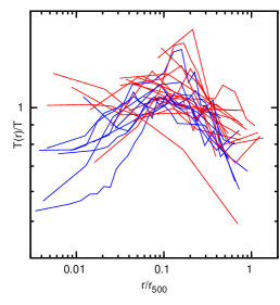
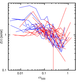
Figure 2: Top row, left to right: Temperature profiles scaled by $r_{500}$ and global temperature (linear), metallicity profiles scaled by $r_{500}$ (linear), surface brightness profiles scaled by $r_{500}$ (logarithmic). Bottom row: Same as above, but all plotted with lines, in logarithmic scale. Groups where a low-temperature core has been removed are shown in blue, others in red.

4.1 Radial Profiles

The projected temperature and metallicity profiles of the group sample are plotted in Fig. 2 (left and center), scaled by $r_{500}$, both in linear and logarithmic scales (top and bottom). In the lower part of the figure the objects where a low-temperature core was removed from the temperature analysis are shown as dotted lines. The temperature profiles behave quite universally for $r\gtrsim 0.05\,r_{500}$, with a flat plateau in the middle and decline beyond $r\sim 0.2r_{500}$. Towards the inner regions however, there is an increase in scatter, and at small radii the profiles vary between being quite flat and showing a clear drop in temperature.

The metallicity profiles have a larger scatter, especially in the outer bins, where $Z$ was not very well constrained by the data, but also show a universal decrease with radius. However objects with a central temperature drop tend to have higher metallicities in the center.

The observed surface brightness profiles are plotted in Fig. 2 (right), scaled by $r_{500}$. Individual temperature, metallicity, and surface brightness profiles are shown in appendix C.

4.2 Scaling Relations

The best-fit results for all relations, including scatter, are listed in Table 4.

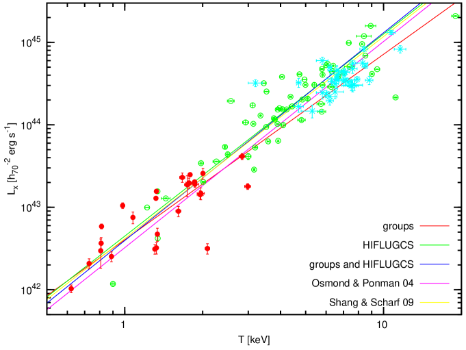
Figure 3: $L_{\text{x}}$-$T$ relation. Filled red circles are groups, open green circles are HIFLUGCS clusters (Reiprich & Böhringer 2002, Hudson et al. 2010), light blue asterisks are LoCuSS clusters (Zhang et al. 2008).

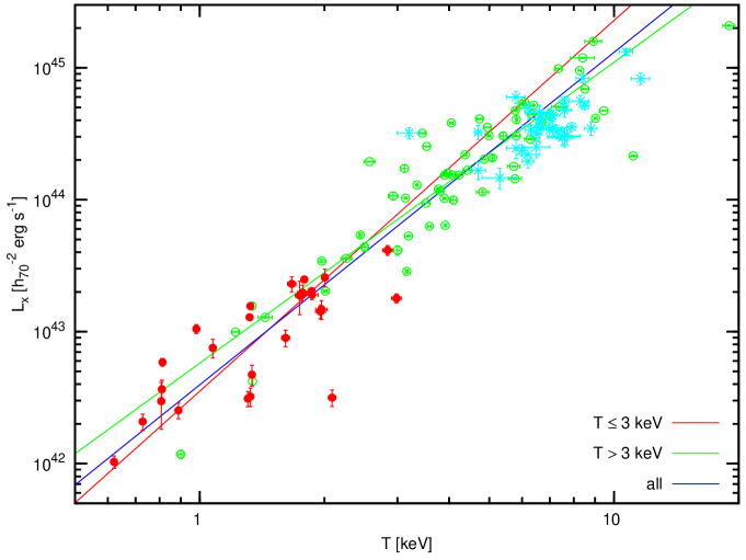
Figure 4: Same points as in Fig. 3, but the fits are cut at $3\,\mathrm{keV}$.

Figure 5: $M_{500}$-$T$ relation. Filled red circles are groups, open green circles are HIFLUGCS clusters, blue open triangles are the groups from Sun et al. (2009), light blue asterisks are LoCuSS clusters.

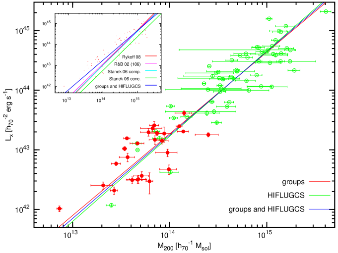
Figure 6: $L_{\text{x}}$-$M_{200}$ relation. Filled red circles are groups and open green circles are HIFLUGCS clusters.

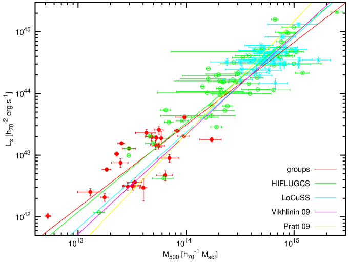
Figure 7: $L_{\text{x}}$-$M_{500}$ relation. Filled red circles are groups, open green circles are HIFLUGCS clusters, and light blue asterisks are LoCuSS clusters.

Table 4: Fit results of all scaling relations

Relation ($Y$-$X$)	Sample	a	b	$\sigma_{\text{tot}}$ (X)	$\sigma_{\text{tot}}$ (Y)	$\sigma_{\text{int}}$ (X)	$\sigma_{\text{int}}$ (Y)
$L_{\text{x}}$-$T$	groups	$2.25\pm 0.21$	$-0.02\pm 0.09$	$0.122$	$0.275$	$0.119$	$0.268$
	HIFLUGCS	$2.45\pm 0.16$	$0.12\pm 0.04$	$0.105$	$0.258$	$0.105$	$0.257$
	groups & HIFLUGCS	$2.52\pm 0.10$	$0.10\pm 0.03$	$0.109$	$0.275$	$0.108$	$0.274$
	$T<3\,\mathrm{keV}$	$2.81\pm 0.27$	$0.19\pm 0.10$	$0.110$	$0.308$	$0.108$	$0.304$
	$T\geq 3\,\mathrm{keV}$	$2.28\pm 0.25$	$0.15\pm 0.06$	$0.107$	$0.243$	$0.106$	$0.242$
$M_{500}$-$T$	groups	$1.68\pm 0.20$	$0.15\pm 0.07$	$0.104$	$0.176$	$0.098$	$0.165$
	HIFLUGCS	$1.70\pm 0.08$	$0.21\pm 0.02$	$0.077$	$0.131$	$0.051$	$0.087$
	groups & HIFLUGCS	$1.75\pm 0.06$	$0.20\pm 0.02$	$0.084$	$0.147$	$0.067$	$0.117$
$M_{2500}$-$T$	groups	$1.59\pm 0.18$	$-0.24\pm 0.06$	$0.097$	$0.154$	$0.093$	$0.147$
$L_{\text{x}}$-$M_{200}$	groups	$1.37\pm 0.20$	$-0.43\pm 0.08$	$0.229$	$0.313$	$0.215$	$0.293$
	HIFLUGCS	$1.43\pm 0.10$	$-0.47\pm 0.08$	$0.211$	$0.301$	$0.186$	$0.265$
	groups & HIFLUGCS	$1.40\pm 0.06$	$-0.45\pm 0.04$	$0.219$	$0.307$	$0.199$	$0.278$
$L_{\text{x}}$-$M_{500}$	groups	$1.34\pm 0.18$	$-0.21\pm 0.09$	$0.226$	$0.303$	$0.214$	$0.287$
	HIFLUGCS	$1.44\pm 0.10$	$-0.18\pm 0.06$	$0.202$	$0.291$	$0.176$	$0.254$
	LoCuSS	$1.55\pm 0.98$	$-0.33\pm 0.76$	$0.167$	$0.259$	$0.099$	$0.153$
	all	$1.44\pm 0.06$	$-0.18\pm 0.04$	$0.209$	$0.301$	$0.189$	$0.272$
$L_{\text{x}}$-$M_{2500}$	groups	$1.42\pm 0.16$	$0.33\pm 0.12$	$0.203$	$0.288$	$0.194$	$0.276$
$M_{500}$-$Y_{\text{x},500}$	groups	$0.53\pm 0.06$	$-0.62\pm 0.05$	$0.369$	$0.194$	$0.350$	$0.184$
	HIFLUGCS	$0.55\pm 0.04$	$-0.63\pm 0.09$	$0.286$	$0.157$	$0.218$	$0.120$
	groups & HIFLUGCS	$0.55\pm 0.02$	$-0.63\pm 0.04$	$0.311$	$0.170$	$0.264$	$0.144$
$M_{2500}$-$Y_{\text{x},2500}$	groups	$0.53\pm 0.05$	$-0.69\pm 0.03$	$0.283$	$0.150$	$0.270$	$0.143$
$L_{\text{x}}$-$Y_{\text{x},500}$	groups	$0.71\pm 0.05$	$-1.05\pm 0.06$	$0.379$	$0.269$	$0.369$	$0.262$
	HIFLUGCS	$0.79\pm 0.03$	$-1.10\pm 0.05$	$0.200$	$0.158$	$0.196$	$0.155$
	groups & HIFLUGCS	$0.78\pm 0.02$	$-1.08\pm 0.05$	$0.261$	$0.203$	$0.257$	$0.200$
$L_{\text{x}}$-$Y_{\text{x},2500}$	groups	$0.76\pm 0.05$	$-0.66\pm 0.05$	$0.336$	$0.256$	$0.327$	$0.249$
$M_{\text{g},500}$-$M_{500}$	groups	$1.38\pm 0.18$	$0.83\pm 0.09$	$0.217$	$0.300$	$0.208$	$0.288$
	HIFLUGCS	$1.26\pm 0.12$	$0.78\pm 0.08$	$0.192$	$0.242$	$0.161$	$0.204$
	groups & HIFLUGCS	$1.28\pm 0.06$	$0.78\pm 0.04$	$0.202$	$0.259$	$0.181$	$0.231$
$M_{\text{g},2500}$-$M_{2500}$	groups	$1.34\pm 0.16$	$0.75\pm 0.11$	$0.175$	$0.235$	$0.169$	$0.227$
$f_{\text{g},500}$-$T$	groups	$1.32\pm 0.32$	$0.11\pm 0.12$	$0.222$	$0.294$	$0.216$	$0.286$
	HIFLUGCS	$0.83\pm 0.42$	$-0.22\pm 0.08$	$0.314$	$0.262$	$0.286$	$0.239$
	groups & HIFLUGCS	$0.79\pm 0.09$	$-0.17\pm 0.03$	$0.337$	$0.268$	$0.315$	$0.250$
$f_{\text{g},2500}$-$T$	groups	$1.12\pm 0.32$	$-0.15\pm 0.12$	$0.226$	$0.253$	$0.222$	$0.249$

• Notes: See section 3.5 for fit functions.

$L_{\text{x}}$-$T$ Relation

The luminosity-temperature relation for the group sample is plotted in Fig. 3, together with the $64$ HIFLUGCS clusters (Hudson et al. 2010) and the $37$ LoCuSS clusters from Zhang et al. (2008). Fitting groups and clusters separately gives a slightly shallower slope for the groups ($2.25\pm 0.21$ compared to $2.45\pm 0.16$ for HIFLUGCS), but they are consistent within the errors. Fitting HIFLUGCS together with the group sample steepens the relation to $2.52\pm 0.10$, but this effect is again not significant considering the uncertainties. The best fit group relation is also in good agreement with both the relations found for the GEMS group sample (Osmond & Ponman 2004) and a local Suzaku cluster sample (Shang & Scharf 2009).

We also investigated whether selecting groups and clusters by temperature produces a different result from the luminosity cut applied before. We applied cuts at different temperatures (stepsize $0.5\,\mathrm{keV}$), and the lowest temperature at which the difference in slope of cooler and hotter objects was significant was $3\,\mathrm{keV}$, so we chose this as a cut. The resulting fits are shown in Fig. 4. We found that systems below $3\,\mathrm{keV}$ follow a significantly steeper relation ($2.81\pm 0.28$) than the hotter systems ($2.28\pm 0.24$).

It is also interesting to note that the groups have higher scatter than the clusters both in $T$ and $L_{\text{x}}$. Similarly, when selecting by temperature the intrinsic scatter in both parameters is higher for the cooler systems ($0.268$ vs. $0.257$ for $L_{\text{x}}$ and $0.119$ vs. $0.105$ for $T$).

We also tried fitting this relation with a broken powerlaw function, but this improves the fit only marginally and the data do not constrain the fit well due to the large scatter.

$M$-$T$ Relation

In Fig. 5 we show the fits to the $M_{500}$-$T$ relation. We again compare the group sample to the HIFLUGCS and the LoCuSS clusters, as well as the group sample of Sun et al. (2009), and the cluster sample of Vikhlinin et al. (2009).

The slopes of all these fits are very similar, and the best fit relations of groups and clusters are consistent with each other ($1.68\pm 0.20$ vs. $1.70\pm 0.08$). However the normalization of our group sample is $\sim 10-30\,\mathrm{\%}$ lower than the others, in particular of the other group sample. Possible reasons for this will be discussed in section 5.

When fitting groups and clusters we once more find a slightly, but not significantly steeper best fit relation ($1.75\pm 0.06$) compared to the pure cluster fit. Again we note that the scatter in groups is larger than in clusters ($0.165$ vs. $0.087$ for $M$ and $0.098$ vs. $0.051$ for $T$).

For $r_{2500}$ we find a best fit $M$-$T$ relation of $a=1.59\pm 0.18$ and $b=-0.24\pm 0.06$.

$L_{\text{x}}$-$M$ Relation

The luminosity-mass relation is plotted in Figs. 6 and 7 (for $M_{200}$ and $M_{500}$, respectively). Note that for our group sample the measurement of $M_{200}$ involved significant extrapolation beyond the actual data. We show the $L_{\text{x}}$-$M_{200}$ relation here primarily for comparison with other publications.

All the three fits are very close together, and the slopes of the group sample and the HIFLUGCS clusters are consistent with each other (in the $L_{\text{x}}$-$M_{200}$ relation $1.37\pm 0.20$ for groups, $1.43\pm 0.10$ for HIFLUGCS). The cluster fit is not changed significantly by including the groups ($1.40\pm 0.06$). The same trend can also be seen for $M_{500}$.

The $L_{\text{x}}$-$M_{200}$ relation of clusters and groups combined is shown together with several other cluster relations in the inset plot of Fig. 6. The fit to the extended HIFLUGCS sample (106 clusters, Reiprich & Böhringer 2002), the stacked relation found by Rykoff et al. (2008), and the compromise model of Stanek et al. (2006) agree very well with each other, while Stanek et al.’s concordance model fit is significantly lower in normalization. See section 5 for a more detailed discussion.

In Fig. 7 we compare the group $L_{\text{x}}$-$M_{500}$ relation to both the HIFLUGCS and LoCuSS clusters, as well as Vikhlinin et al. (2009) and Pratt et al. (2009). The group relation is shallower than all these cluster samples but consistent with HIFLUGCS (see discussion).

Once more we find the intrinsic scatter for groups to be larger than for the cluster samples, for instance the scatter in $M_{500}$ is $0.287$ for the groups, but only $0.254$ for HIFLUGCS and $0.153$ for LoCuSS.

The best fit $L_{\text{x}}$-$M$ relation for $r_{2500}$ is $a=1.42\pm 0.16$ and $b=0.33\pm 0.12$.

$Y_{\text{x}}$, $M_{\text{g}}$ and $f_{\text{g}}$ Relations

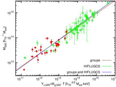
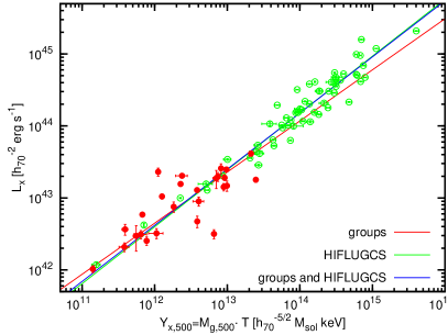
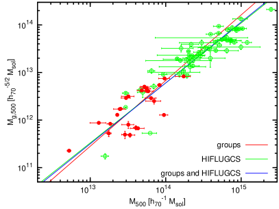
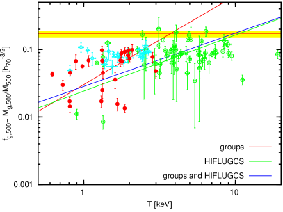
Figure 8: $Y_{\text{x}}$ and gas fraction relations at $r_{500}$. Top left: $M$-$Y_{\text{x}}$ relation. Top right: $L_{\text{x}}$-$Y_{\text{x}}$ relation. Lower left: $M_{\text{g}}$-$M$ relation. Lower right: $f_{\text{g}}$-$T$ relation. Filled red circles are groups, open green circles are HIFLUGCS clusters (gas masses from Zhang et al. 2011), and light blue asterisks are the groups from Sun et al. (2009). The orange line with yellow error regions is the cosmic baryon fraction from WMAP5 (Dunkley et al. 2009).

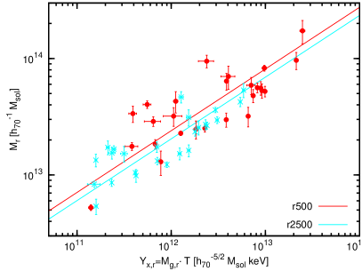
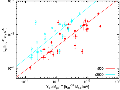
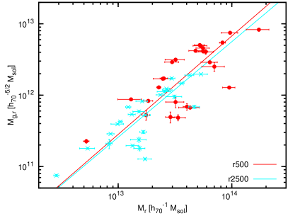
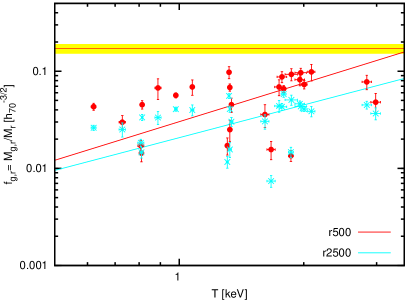
Figure 9: Same relations as in Fig. 8, but at different radii. Filled red circles are for $r=r_{500}$ and light blue asterisks are for $r=r_{2500}$.

In Fig. 8 we show fit results to the $M$-$Y_{\text{x}}$, $L_{\text{x}}$-$Y_{\text{x}}$, $M_{\text{g}}$-$M$, and $f_{\text{g}}$-$T$ relations, all determined for $r_{500}$. We compare the group results to the HIFLUGCS clusters (gas masses were measured by Zhang et al. 2011 for all except 2A0335, which is omitted here). The gas mass fractions of Sun et al.’s group sample and the cosmic baryon fraction $\Omega_{\text{b}}/\Omega_{\text{m}}$ measured from WMAP five-year data (Dunkley et al. 2009) are also included in the $f_{\text{g}}$-$T$ plot for comparison.

For the $M$-$Y_{\text{x}}$ and $L_{\text{x}}$-$Y_{\text{x}}$ relations, the different samples are in good agreement, although the slope of the fit is slightly flatter for the groups than for the clusters ($0.53\pm 0.06$ vs. $0.55\pm 0.04$ and $0.71\pm 0.05$ vs. $0.79\pm 0.03$, respectively). The $M_{\text{g}}$-$M$ relation for groups is a bit steeper than that of the clusters, but the slopes are consistent with each other within the uncertainties ($1.38\pm 0.18$ vs. $1.26\pm 0.12$).

The intrinsic scatter for these relations is much larger in groups, for example in the $L_{\text{x}}$-$Y_{\text{x}}$ relation, $Y_{\text{x}}$ has a scatter of $0.369$ for the groups, compared to $0.196$ for HIFLUGCS, and similar trends can be seen for the other parameters and relations. Including groups in the fit does not significantly influence any of the cluster relations, for instance the best fit HIFLUGCS $M$-$Y_{\text{x}}$ relation is $a=0.55\pm 0.04$ and $b=-0.63\pm 0.09$, compared to $a=0.55\pm 0.02$ and $b=-0.63\pm 0.04$ of the combined fit, and the difference is negligible for the $L_{\text{x}}$-$Y_{\text{x}}$ and $M_{\text{g}}$-$M$ relations as well.

There is a strong trend for lower $f_{\text{g}}$ at lower temperatures. The slope of the group $f_{\text{g}}$-$T$ relation is clearly different from zero ($1.32\pm 0.32$), as are the shallower fit to the HIFLUGCS clusters ($0.83\pm 0.42$), and the combined fit of groups and clusters ($0.79\pm 0.09$). The intrinsic scatter in $f_{\text{g}}$ is larger for the group sample than for HIFLUGCS ($0.286$ vs. $0.239$, but it is smaller for $T$ ($0.216$ vs. $0.286$).

In Fig. 9 we show the same relations as before, but compare the radii $r_{500}$ and $r_{2500}$. The relations measured out to $r_{2500}$ have smaller uncertainties and scatter, compared to $r_{500}$.

The gas mass fractions within $r_{2500}$ are typically lower than within $r_{500}$, and the slope of the $f_{\text{g}}$-$T$ relation measured within $r_{2500}$ is flatter than for $r_{500}$, but also significantly differs from zero ($1.12\pm 0.32$).

We have inspected the other scaling relations in terms of $f_{\text{g}}$ but did not find any particular trends for low or high gas mass objects to behave differently. As an example, in Fig. 11 (left) we show the $L_{\text{x}}$-$T$ relation with objects with gas mass fractions above and below the mean marked as different symbols.

4.3 Morphology and Cool Cores

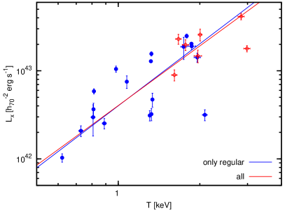
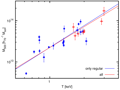
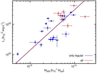
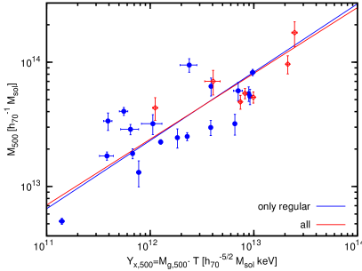
Figure 10: Scaling relations fit using different morphological selections. Filled blue circles are regular (relaxed) objects, open red diamonds are irregular (unrelaxed). Top left: $L_{\text{x}}$-$T$. Top right: $M$-$T$. Lower left: $L_{\text{x}}$-$M$. Lower right: $M$-$Y_{\text{x}}$.

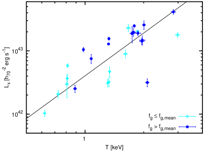
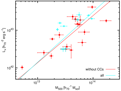
Figure 11: Left: $L_{\text{x}}$-$T$ relation, objects with gas mass fraction above and below the mean value are plotted as different symbols (lower $f_{\text{g}}$ are light blue open diamonds, others are filled blue circles). Right: $L_{\text{x}}$-$M$ relation, comparison of fit with and without cool core objects (light blue open diamonds).

Table 5: Fit results selected by morphology and excluding cool core objects.

Relation ($Y$-$X$)	Sample	a	b	$\sigma_{\text{tot}}$ (X)	$\sigma_{\text{tot}}$ (Y)	$\sigma_{\text{int}}$ (X)	$\sigma_{\text{int}}$ (Y)
$L_{\text{x}}$-$T$	regular	$2.34\pm 0.32$	$0.02\pm 0.16$	$0.128$	$0.300$	$0.126$	$0.294$
	without CCs	$2.03\pm 0.22$	$-0.13\pm 0.11$	$0.125$	$0.255$	$0.121$	$0.245$
	all	$2.25\pm 0.21$	$-0.02\pm 0.09$	$0.122$	$0.275$	$0.119$	$0.268$
$M_{500}$-$T$	regular	$1.76\pm 0.29$	$0.19\pm 0.12$	$0.112$	$0.197$	$0.107$	$0.189$
	without CCs	$1.63\pm 0.24$	$0.14\pm 0.08$	$0.122$	$0.199$	$0.115$	$0.187$
	all	$1.68\pm 0.20$	$0.15\pm 0.07$	$0.104$	$0.176$	$0.098$	$0.165$
$L_{\text{x}}$-$M_{500}$	regular	$1.34\pm 0.19$	$-0.22\pm 0.11$	$0.222$	$0.298$	$0.211$	$0.283$
	without CCs	$1.25\pm 0.22$	$-0.31\pm 0.12$	$0.230$	$0.287$	$0.214$	$0.267$
	all	$1.34\pm 0.18$	$-0.21\pm 0.09$	$0.226$	$0.303$	$0.214$	$0.287$
$M_{500}$-$Y_{\text{x},500}$	regular	$0.55\pm 0.08$	$-0.63\pm 0.05$	$0.383$	$0.210$	$0.369$	$0.202$
	without CCs	$0.52\pm 0.07$	$-0.62\pm 0.06$	$0.374$	$0.196$	$0.351$	$0.184$
	all	$0.53\pm 0.06$	$-0.62\pm 0.05$	$0.369$	$0.194$	$0.350$	$0.184$
$f_{g,500}$-$T$	regular	$1.45\pm 0.62$	$0.22\pm 0.26$	$0.203$	$0.294$	$0.198$	$0.286$
	without CCs	$1.18\pm 0.28$	$0.08\pm 0.11$	$0.218$	$0.258$	$0.209$	$0.247$
	all	$1.32\pm 0.32$	$0.11\pm 0.12$	$0.222$	$0.294$	$0.216$	$0.286$

We also tested several scaling relations for a possible influence of morphology and dynamical state, using the selection criteria introduced in section 3.6. We compared the whole sample to one where unrelaxed objects are excluded, and to one where the cool core objects are excluded. Table 5 contains the best-fit results for the $L_{\text{x}}$-$T$, $M$-$T$, $L_{\text{x}}$-$M$, and $M$-$Y_{\text{x}}$ relations, plotted in Fig. 10 for the morphology selection, as well as the $f_{\text{g}}$-$T$ relation.

We found that the morphology selection had no significant effect on any of these relations. For all relations the fit for regular systems has the larger uncertainty, mainly because there are fewer objects constraining the fit. There is however a trend for these objects to be hotter, e. g. none of the unrelaxed groups has a temperature below $1.5\,\mathrm{keV}$. Merging systems are not scattered significantly more strongly than groups that appear to be regular, and excluding disturbed systems only slightly improves the scatter in the $L_{\text{x}}$-$M$ and the $f_{\text{g}}$-$T$ relations, while in the other relations the scatter actually increases, probably due to statistics. For example, the $M$-$T$ relation fit using only regular groups has an intrinsic scatter of $0.189$ in $M$ and $0.107$ in $T$, while for the complete relation the scatter is only $0.165$ and $0.098$, respectively.

We also compared the best-fit relations to the fits excluding objects with a cool core, in order to determine whether cool cores have an effect on global properties apart from the temperature (where cool cores have been excluded). The results are again shown in Table 5. We found that the cool cores do not significantly affect the relations, the largest impact is on the luminosity-temperature relation, which is flatter when the CC objects are excluded ($2.03\pm 0.22$ compared to $2.25\pm 0.21$), but the changes are not significant within the uncertainties. The $L_{\text{x}}$-$M$ relation is shown as an example in Fig. 11 (right), as a relation that does not explicitly contain $T$. Here the fits are also consistent within the errorbars ($a=1.25\pm 0.22$ and $b=-0.31\pm 0.12$ vs. $a=1.34\pm 0.18$ and $b=-0.21\pm 0.09$ for the full sample). The main effect of excluding cool core objects is reducing the scatter in $L_{\text{x}}$ (from $0.287$ to $0.267$ in the $L_{\text{x}}$-$M$ relation) and $f_{\text{g}}$ (from $0.286$ to $0.247$ in the $f_{\text{g}}$-$T$ relation). We observe that objects with a cool core tend to have a higher luminosity, for instance the mean $\Delta L_{\text{x}}=\log L_{\text{x}}-\left(a\cdot\log T+b\right)$ is $0.08$ for the cool core objects and $-0.04$ for the others, meaning the CC objects mostly lie above the $L_{\text{x}}$-$T$ relation. This is a well-known phenomenon, but apart from this they do not particularly stand out in any of the scaling relations.

5 Discussion

In section 4.1 we have shown universal behavior in the radial temperature and metallicity profiles scaled to a characteristic radius. However, there is an increase in scatter and a large variability in the inner parts of the temperature profiles ($\lesssim 0.05r_{500}$), where some groups exhibit a drop in temperature while others appear to remain flat down to the very center. A variability of the inner temperature slopes has also been observed in the HIFLUGCS clusters, by Hudson et al. (2010). It is difficult to say whether this is due to the cool core/non-cool core bimodality often reported for clusters, since the profiles have only a small number of radial bins and in many cases do not extend down to the very center. Unfortunately, this is a typical problem when analyzing groups, as the profiles cannot be resolved as finely as in clusters, due to the much lower count rates even at the center, and the low signal to noise in the outskirts. Those profiles that do resolve the core however have clear trends for either constant temperature or a cool core. It is possible that the bimodality is either not as pronounced in groups as it is in clusters, or it is simply not clearly detectable in this sample because of the low count rates and would require more data with longer exposure times.

With regards to a systematic difference or “break” in the scaling relations due to feedback or other non-gravitational processes, our results are somewhat ambiguous (see section 4.2). When comparing fits of the group sample with cluster relations we found that in virtually all parameters the intrinsic scatter is larger for groups, while the slopes of the scaling relations are still consistent with the cluster fits. The strong temperature-dependence of the gas mass fraction however indicates a systematic difference in the physical properties of clusters and groups. If groups generally have lower $f_{\text{g}}$ one would expect to see a stronger influence of the galactic component on the whole system and especially the central region via AGN feedback, compared to clusters, where the ICM component is dominant over the galaxies in terms of mass.

Our data do not show a clear break in a broken powerlaw sense, but the scaling relations are not completely consistent either. It is possible there is a gradual, continuous shift which may be harder to detect due to the increase in scatter, and which leads to different results depending on which objects are compared. For example, we found that the $L_{\text{x}}$-$T$ slope of our group sample selected by luminosity is consistent with that of the HIFLUGCS clusters, as well as the samples of Osmond & Ponman (2004) and Shang & Scharf (2009), but the relation for systems below $3\,\mathrm{keV}$ is steeper than the slope for hotter objects. Using a broken powerlaw function however does not significantly improve the fit. Fitting the groups together with the clusters steepens the $L_{\text{x}}$-$T$ as well as the $M$-$T$ relation in comparison to the pure cluster fits, which is in agreement with the findings of e. g.  Finoguenov et al. (2001). However the best-fit normalization for groups is rather low, especially of the $M$-$T$ relation, and this may be sufficient to cause the observed steepening.

In section 4.2 we have noted that the normalization of our $M_{500}$-$T$ relation is $\lesssim 30\,\mathrm{\%}$ lower than, among others, the relation found by Vikhlinin et al. (2009). However these authors used the $Y_{\text{x}}$-$M$ relation to estimate their masses, and their sampling only goes down to temperatures of $\sim 2.5\,\mathrm{keV}$. But our $M$-$T$ normalization is still lower than a comparable group relation obtained by Sun et al. (2009), which is based solely on Chandra data, like our sample. This discrepancy could be caused by a multitude of effects, some of which we will briefly discuss here.

Probably the most important known bias on the $M$-$T$ relation due to selection is based on the difference between relaxed and unrelaxed systems. As mentioned in the introduction, simulations indicate that for a given mass merging clusters are observed to be cooler than relaxed clusters, due to gas that has not yet been thermalized (e. g. Mathiesen & Evrard 2001, Ventimiglia et al. 2008). Sun et al.’s and Vikhlinin et al.’s samples are explicitly selected to be relaxed, while our groups were not subjected to any selection by morphology or dynamical state. However, following this chain of reasoning our groups should be cooler than the others, not hotter, so this cannot be the explanation. On the other hand, it is possible that this sample is missing some of the fainter, cooler objects due to flux limits and archive bias, and by chance appears to have an offset from the other samples.

Another possible reason why observed group properties differ from cluster scaling relations could be the limited radial extent out to which group emission can be measured (e. g. Mulchaey 2000). While group emission is in theory detectable out to large radii, the gas is emitting at very low temperatures ($\lesssim 0.5\,\mathrm{keV}$) and hard to distinguish from the Galactic foreground, which is similar in terms of both surface brightness and temperature. In addition, our analysis is limited by Chandra’s field-of-view. Due to these limitations, our profiles could only be traced out to $\sim 0.7r_{500}$ on the average. There has been some computational and observational evidence indicating that SBPs steepen at large radii, even more strongly than a double $\beta$-model accounts for (e. g. Vikhlinin et al. 2006), which could bias low our mass measurements. This would however not explain an offset between our results and other work that relies on Chandra data as well, like Sun et al. (2009). Furthermore, other investigators have found the cluster density profiles to be consistent with (Humphrey et al. 2011) or even flatter than predictions (Kawaharada et al. 2010, Simionescu et al. 2011, Urban et al. 2011).

Fortunately there is some overlap between our groups and those of Sun et al. (2009) and also Gastaldello et al. (2007). Seven of our groups are present in the former sample, and six in the latter, so we can perform a quantitative direct comparison between the results of the different temperature and mass measurements. When comparing $T$ values for the groups overlapping with Sun et al.’s work (Gastaldello et al. have not published temperatures for their sample), we found that on average our temperatures are in agreement ($10^{\langle\log T-\log T_{\text{Sun}}\rangle}=1.09^{+0.13}_{-0.12}$). Differences in the individual cluster temperatures may be caused by the different temperature determinations applied. While we fitted the (projected) global temperature using the whole observed area, Sun et al. used the deprojection method developed by Vikhlinin et al. (2006a and 2006b) to fit 3D temperature profiles. This method is likely to yield lower temperatures because it puts more weight on cooler gas components at large radii. Sun et al. excluded the inner core regions $<0.15\,r_{500}$, which is comparable to our cuts, so we do not expect cool gas at the group centers to make a large difference. It is possible however that the different background treatments (blank-sky vs. stowed background files) also have an effect on the temperature measurements.

When comparing the masses, we find that our values are again consistent with other work ($10^{\langle\log M-\log M_{\text{Sun}}\rangle}=1.10^{+0.87}_{-0.49}$ and $10^{\langle\log M-\log M_{\text{Gastaldello}}\rangle}=0.99^{+0.61}_{-0.38}$, respectively), albeit with quite large statistical spread. So we conclude that since the individual mass and temperature values are consistent the difference in normalization of the $M$-$T$ relation is most likely caused by incompleteness of the samples and/or the high scatter in properties of galaxy groups. We also point out that the combined fit of the groups with the HIFLUGCS clusters is in good agreement with the other relations.

Of the scaling relations investigated here, the relation between luminosity and mass is the most useful for future cluster cataloguing missions like eROSITA. For tens of thousands of new detections $L_{\text{x}}$ is the easiest X-ray property to measure, and which can be determined from even a small number of photons. In this context it is convenient that our results indicate that the cluster relation holds also for low-mass objects. The best fit $L_{\text{x}}$-$M_{500}$ relation for groups in the low-mass range agrees well with the HIFLUGCS cluster relation, while being shallower than the fit found for the LoCuSS clusters, as well as the relations found by Vikhlinin et al. (2009) and Pratt et al. (2009). However we point out that the LoCuSS clusters all lie in a narrow range both in luminosity and mass and therefore by themselves cannot constrain the slope of the $L_{\text{x}}$-$M$ relation very well, and the authors of the latter two publications did not measure the masses individually but estimated $M_{500}$ from the $Y_{\text{x}}$-$M$ relation.

For comparison with previous publications we also show our results for the $L_{\text{x}}$-$M_{200}$ relations, although the temperature and surface brightness profiles had to be extrapolated considerably to determine the mass within $r_{200}$ and we expect the uncertainties to be large. Again we found reasonable agreement between the group relation and HIFLUGCS, as well as the relations found by Stanek et al. (2006, compromise model) and Rykoff et al. (2008). Stanek et al.’s concordance model appears to significantly underestimate the normalization, which can be explained by the difference in the assumed cosmological models, as has been argued by Reiprich (2006).

The $M$-$Y_{\text{x}}$, $L_{\text{x}}$-$Y_{\text{x}}$, and $M_{\text{g}}$-$M$ relations also are consistent for groups and clusters, although the scatter is much larger for groups. Including groups into the relations does not change the fits of the HIFLUGCS clusters.

We observed a strong correlation between temperature and gas mass fraction, which is in agreement with e. g. Reiprich (2001), Gastaldello et al. (2007), and Pratt et al. (2009), and could explain naturally why the X-ray emitting gas in groups can only be traced out to smaller physical radii than in clusters. The measured group gas fractions are also lower than the typical cluster $f_{\text{g}}$ around $0.1$ (e. g. Vikhlinin et al. 2009a). Sun et al. (2009) pointed out this may be caused by a central drop in $f_{\text{g}}$, and might not be a global effect. This is in in principle in agreement with our finding that the gas fraction increases with radius, which should be considered when using $f_{\text{g}}$ to determine cosmological parameters. We also find the $f_{\text{g}}$-$T$ relation within $r_{2500}$ to be significantly different from constant, although the slope is flatter than for $r_{500}$.

We have quantitatively confirmed the expectation that, compared to clusters, groups have a larger intrinsic scatter in properties such as luminosity or temperature, which clearly exceeds the statistical uncertainties. This increases the scatter in derived parameters like total mass and even the $Y_{\text{x}}$ parameter, which for clusters is thought to be the most robust against scatter due to merger activity. But for our sample the $Y_{\text{x}}$ scaling relations the scatter is not reduced compared to other relations, but is even actually larger. Interestingly, in the $f_{\text{g}}$-$T$ relation the scatter in $T$ was actually quite a bit lower for the group sample than for the clusters, but not for $f_{\text{g}}$. We assume this is an effect of the much steeper slope.

We did not find dynamical state and morphology to have any significant effect on the relations, and merging objects are apparently not responsible for the large scatter. Concerning the impact of cool cores, by excluding the core region in the temperature analysis we have in principle removed any possible bias on temperature. On the other hand it was not feasable to remove the cores from the luminosity measurements. The original ROSAT observations have a low spatial resolution, comparable to the core regions removed for the temperature determination in our analysis, and Chandra data do not extend out to $r_{500}$ due to the small field of view. In addition, for the purpose of applying our relation to, for example, eROSITA, excluding the centers would not necessarily be useful since the clusters we compare our relation to will not have the cores removed, either.

Overall, we found that objects with a central temperature drop tend to have higher luminosities and lie above for instance the $L_{\text{x}}$-$T$ relation. This is not surprising since cool, dense gas produces the most X-rays and consequently cool cores clusters are generally found to be brighter than non-cool cores, and are more likely to be detected. Excluding the cool core objects from the fits has however not significantly changed the best fit results for our scaling relations (see section 4.3).

Therefore it seems more likely that scatter due to baryonic physics in the core regions, and not substructure and merger bias, is responsible for the large uncertainties in the fit results. For instance, the X-ray luminosities have been measured without applying any core exclusion and thus may be subject to large scatter due to galactic influences like AGN feedback. While this holds true for both the groups and the HIFLUGCS clusters, it is possible either that core properties are generally more variable in groups, or that any variation in the strength of feedback processes such as heating has a stronger impact on cooler systems with lower gas masses (e. g. Mittal et al. 2011). The latter argument could explain both the increased scatter and the steepening of the $L$-$T$ relation for objects with $T<3\,\mathrm{keV}$.

We note that properties measured out to $r_{2500}$ have systematically lower scatter than those determined out to $r_{500}$. This is not surprising, since the necessary extrapolations add a large uncertainty to the measurements, because it is not possible to reliably measure whether group profiles at large radii are shaped like cluster profiles or perhaps drop off more quickly. These limits may be improved by including more data into the analysis, for instance observations taken with XMM-Newton or Suzaku.

A comparison between groups and clusters in addition depends on the criteria used to distinguish the two classes, as the transition is a smooth one. We compiled our group sample using a luminosity limit, but for instance for the $L_{\text{x}}$-$T$ relation we found more conclusive results when dividing the objects by temperature, perhaps partly due to the higher scatter in $L_{\text{x}}$ for the cooler systems. This indicates differences in selection criteria may be a reason why different authors find inconsistent and even contradictory results. Therefore it could be useful, but is beyond the scope of this paper, to test and compare a number of selection parameters, such as temperature, luminosity, velocity dispersion, richness, virial radius, gas mass, or total mass. In the next section, we test the influence of luminosity, flux, and redshift cuts on our sample.

5.1 Selection Effects

Figure 12: Observed $L_{\text{x}}$-$T$ relation and “true” relation according to Monte Carlo simulations.

Since our sample is derived from flux-limited parent samples, we expect our results to be susceptible to Malmquist bias, and perhaps also “archival bias.” Another possible selection bias may result from the luminosity cut applied in the construction of the group sample, since systems scattered above the luminosity limit are excluded, effectively placing more weight on fainter objects. However these effects cannot be properly corrected for in a sample that is incomplete, as is the case for our and most other published samples. We hope to overcome these biases by using a statistically complete sample, but even with this incomplete sample we can make an estimation of how large an effect the Malmquist bias has on the scaling relations, as well as the cuts in $L_{\text{x}}$ and $z$. We performed this test for the luminosity-temperature relation, following a similar procedure as described in Mittal et al. (2011).

Malmquist bias is caused by the fact that using a flux limit to select a sample of objects favors bright objects because of intrinsic scatter. In order to measure this effect and the other aforementioned biases for our sample we created a simulated group sample and iteratively varied the input $L_{\text{x}}$-$T$ slope and normalization until the fake data reproduced the observed relation. For this we first created a mock cluster sample in the redshift range of 0.01 to 0.2, such that the number of objects grew as luminosity distance $D_{\text{L}}$ cubed, corresponding to a random homogeneous distribution in a spherical volume with radius $D_{\text{L}}$. We then used the powerlaw temperature function measured by Markevitch (1998) to assign temperatures to the objects, in the range $0.5-10\,\mathrm{keV}$. These temperatures were converted to luminosities using the respective $L_{\text{x}}$-$T$ relation to be tested, and applying the measured intrinsic and statistical scatter (we did not consider evolution effects, since our sample is nearby). We then applied a flux cut of $2.5\cdot 10^{-12}\,\mathrm{erg\,s^{-1}\,cm^{-2}}$ and a luminosity cut of $L_{\text{x}}<2.55\cdot 10^{43}\,h^{-2}_{70}\,\mathrm{erg\,s^{-1}}$, to reproduce the selections made for the actual group sample. The total number of objects was chosen such that after the cuts the sample had on average the same number of objects as the real sample ($\sim 20-30$).

The input $L_{\text{x}}$-$T$ parameters that produced the measured relation ($a=2.25$, $b=-0.02$) are $a=2.70$ and $b=0.03$. This means that the observed relation is higher in normalization in the range in which our group sample lies (see Fig. 12), which is what is expected due to Malmquist bias. The observed relation is also flatter, which is probably an effect of the luminosity cut mentioned above. However at this point we cannot reliably correct for these biases since the sample is not statistically complete. For the purpose of comparing groups and clusters this implies that if the flattening due to the luminosity cut is a significant influence the actual group $L_{\text{x}}$-$T$ relation could actually be steeper than the cluster relation. This would also be supported by our observation that applying a temperature cut instead of the luminosity cut results in a significantly steeper group relation (see section 4.2).

5.2 Note on Model Choice

We discuss briefly to what extent different model choices affect the final mass result, and justify the direct comparison to the HIFLUGCS measurements. We found, in agreement with Xue & Wu (2000a), that fitting a double $\beta$-model instead of a single one results in, on the average, higher values of $\beta$ and hence higher masses. In most cases the double model gives a much better and more accurate fit because it uses separate components to describe the central region, which may have excess emission from a cooling core, and the outer parts, which are more representative of the overall density gradient.

We note that on the other hand including the temperature gradient decreases the mass compared to the isothermal model. We found the mass values determined using the single $\beta$ and isothermal model are on average lower than the double $\beta$-model with the temperature gradient by a factor of $10^{\langle\log M_{1\beta\text{, iso}}-\log M_{2\beta\text{, d}T}\rangle}=0.88^{+0.88}_{-0.44}$, which is consistent with unity. In addition we have confirmed that the best-fit slopes for the $L$-$M$ relation are consistent within the errors.

In particular, we argue our mass measurements can be compared to the HIFLUGCS masses from Reiprich & Böhringer (2002), even though these were determined assuming an isothermal profile, fit with single $\beta$-models only. On the other hand, our masses are mostly calculated with double $\beta$-models, taking into account the temperature gradients. This is the same procedure as applied for the LoCuSS clusters (Zhang et al. 08), which we also include in the plots for comparison.

6 Summary and Conclusions

Using a luminosity limit of $L_{\text{x}}<2.55\cdot 10^{43}\,h^{-2}_{70}\,\mathrm{erg\,s^{-1}}$ and a redshift cut of $z>0.01$, we have compiled a statistically complete sample of X-ray galaxy groups with the goal of investigating a possible “break” between scaling relations of groups and clusters, which are important cosmological tools. For this work, we have reduced and analyzed Chandra observations for a subsample of 26 groups, extracted radial temperature, metallicity, and surface brightness profiles, and determined the global temperature, metallicity, total mass, gas mass, gas mass fraction, and $Y_{\text{x}}$ parameter for each object. We have investigated the $L_{\text{x}}$-$T$, $M$-$T$, $L_{\text{x}}$-$M$, $M_{\text{g}}$-$M$, $M$-$Y_{\text{x}}$, $L_{\text{x}}$-$Y_{\text{x}}$, and $f_{\text{g}}$-$T$ scaling relations, and compared these to several cluster relations. We summarize our results as follows:

1. The group temperature profiles scaled to $r_{500}$ decrease universally beyond a radius of $\gtrsim 0.05\,r_{500}$, with larger scatter in the central regions.

2. The $L_{\text{x}}$-$T$ and $M$-$T$ relations are consistent for groups and clusters, with a slight steepening when groups and clusters are fitted together, in agreement with e. g. Finoguenov et al. (2001). Our $M$-$T$ normalization appears to be a bit lower than other comparable work, but on average our results are consistent and we attribute the offset to mainly scatter and selection effects.

3. The most useful relation to estimate masses for large cluster samples, $L_{\text{x}}$-$M$, is also found to be consistent within the errors for both groups and clusters.

4. The $L_{\text{x}}$-$T$ relation is steeper for groups selected via a temperature cut at $T<3\,\mathrm{keV}$, compared to hotter objects. This could indicate that cooler systems are more strongly affected by heating processes such as AGN feedback, supernovae, or cosmic rays.

5. We found a systematic drop of $f_{\text{g}}$ with temperature, significantly different from a constant relation, both within $r_{2500}$ and $r_{500}$. The gas fractions are lower than typical values for clusters ($\sim 0.1$, e. g. Vikhlinin et al. 2009a). The gas mass fractions are also lower at smaller radii, in agreement with the findings of Sun et al. (2009).

6. Groups generally have large scatter in all parameters and large uncertainties where radial profiles had to be extrapolated, which increases the uncertainties on the best-fit relations. This may be improved by including more objects and completing the group sample, and including more data, for instance taken with XMM-Newton or Suzaku.

7. Dynamical state and cool cores have no significant effect on any of the scaling relations. This indicates that merging activity, dynamical state and cool cores do not have as strong an impact on groups as on high-mass systems, and the large scatter is probably due to a different effect, for instance the increasing influence of the galactic component on the ICM.

8. A quantitative test of the impact of selection effects on the $L_{\text{x}}$-$T$ relation showed that the observed group relation is higher in normalization and flatter than the actual relation. We argue that these effects are caused by Malmquist bias and the upper luminosity cut, respectively. However to reliably correct for these effects a statistically complete sample is necessary.

In short, we have found some evidence for a systematic difference between the group and cluster regimes, however the most commonly used scaling relations do not seem to be strongly affected by this. The strongest effects appear to be the lower gas fractions which points to a less dominant role of the ICM in groups than in clusters and stronger influence of the galaxies, and the significantly larger scatter in all relations, which is likely not caused by merging and irregularity, but rather by non-gravitational galactic physics in the core. This large scatter on group properties is highly problematic, as it may generate spurious effects or mask out actual trends. We did not find a hard powerlaw “break”, but it is possible that there is a gradual change that is obscured by the scatter, and by bias due to selection effects. Therefore we will work to continue completing our sample, to be able to eliminate selection biases and to produce more conclusive results.

Appendix A Notes on Individual Groups

A0160

This group/poor cluster of galaxies was classified as “intermediate type” because there is a distinct sub-peak to the east of the center of extended emission. However this sub-peak was excluded from our analysis of the ICM, as it appears not to be interacting with the surrounding material. There is a large degeneracy between temperature and normalization in the spectral fits, so the total error on the surface brightness was overestimated. We corrected for this unreasonably high uncertainty by choosing the smaller of the two errors.

This system was investigated by Drake et al. (2000), who found “wake”-like structures in the X-ray emission, which they interpreted as evidence for ram-pressure stripping of the cluster galaxies by the surrounding ICM.

Jetha et al. (2005) also inspected radio observations for this object, and found a spatial correlation between a wide angle tailed radio galaxy in the BCG and structures in the X-ray emitting gas. They concluded that the secondary peak (“source 1”) corresponds to a large elliptical at slightly higher redshift than the cluster, which they found not to be interacting with the cluster.

HCG62

This group has been studied extensively, in radio, X-ray and optical bands. In the innermost regions, the emission shows traces of dynamical activity, although the overall shape is quite regular. We used only the newer two of the four available Chandra observations, because they are from a more recent different background epoch and together have $\sim 120\,\mathrm{ks}$ of exposure, which is more than sufficient for our analysis.

Using ASCA data, Fukazawa et al. (2001) and Nakazawa et al. (2007) reported an excess of hard emission in the spectra of this group. This hard excess could however not be confirmed by a more recent Suzaku observation (Tokoi et al. 2008).

Spavone et al. (2006) concentrated specifically on the brightest group member, NGC4778, which shows distinct kinematical and morphological peculiarities, which they argued is an indication for a possible recent minor merger event. If this conclusion is correct, the group may still be dynamically disturbed, even though the emission appears to be spherical at large radii.

Two X-ray cavities in this group were studied by Morita et al. (2006), but found no clear explanation for their origin. These authors also found some evidence for a departure from hydrostatic equilibrium in this system. They used a triple $\beta$-model to describe the SBP.

Gu et al. (2007) identified an arc-shaped region spanning from south to northwest, with an average metal abundance about a factor of two higher than the surrounding regions. They concluded this may have been created by AGN activity, or by a recent merger, in accordance with Spavone et al.

Gitti et al. (2010) combined X-ray data from Chandra and XMM-Newton with GMRT radio data and detect low-frequency radio emission associated with the X-ray cavities.

IC1262

This poor cluster appears quite regular and relaxed in the overall emission but shows some remarkable filamentary emission features close to the center which are clearly visible in the Chandra image.

Hudson et al. (2003) first reported a possible detection of a diffuse non-thermal component, measured with Beppo-SAX, which might also correspond to excess emission in radio. Hudson & Henriksen (2003) confirmed this observation with Chandra data, and concluded this cluster has recently merged with a smaller subclump, triggering the non-thermal emission by relativistic shocks.

On the other hand, Trinchieri et al. (2007) found the filamentary structures to be actually cooler than the surrounding regions, and rejected the shock front scenario proposed by Hudson & Henriksen. They suggested these structures may have been formed by ram pressure stripping of a nearby spiral galaxy or a past radio source that has since faded and is now only a relic.

IC1633

This system is the hottest ($T\sim 3\,\mathrm{keV}$) and most massive ($M_{200}\sim 16\cdot 10^{13}\leavevmode\nobreak\ h^{-1}_{70}\leavevmode\nobreak\ M_{\odot}$) object in the sample presented here.

IC4296

This group is the faintest object in our sample, and in addition was observed with only half of the area of the CCD chips (“1/2 subarray mode”) to avoid pile-up, apparently because the observers were interested mostly in the giant radio-active elliptical galaxy at the center (Pellegrini et al. 2003). However, with this configuration large parts of the extended group emission are lost, so both observations essentially are useless for investigating the ICM. We nevertheless performed the analysis, but the object was an obvious outlier in all of the investigated scaling relations, with too high temperature and mass, clearly outside the normal scatter, so it was ultimately excluded from the fits, although it still appears in some of the tables.

MKW4

Using XMM-Newton observations, O’Sullivan et al. (2003) studied this poor HIFLUGCS cluster and found a central temperature gradient lacking strong cooling activity, as well as a sharp abundance peak at the cluster core, located at the position of the central cD galaxy NGC4073. They argued that this system is close to establishing hydrostatic equilibrium and has developed a central temperature drop, but not yet a cooling flow.

Fukazawa et al. (2004) observed this group with Chandra and also found a central temperature drop and high central abundance. They attributed this high abundance to the weakness of the AGN in the cD galaxy, which allowed the ejected metals to remain near the cluster center.

MKW8

This poor cluster is the brightest object in our sample, as well as the second hottest. It is also included in the HIFLUGCS sample. The X-ray map is slightly asymmetric, and in the optical image there are two large galaxies visible at the center.

Hwang et al. (1999) investigated the properties of a small sample of groups and found MKW8 to be a dynamically complex system with a relatively low velocity dispersion.

NGC326

The radio-active central galaxy of this system has an inversion symmetric (“Z”-shaped) morphology and has been studied in the radio regime by Murgia et al. (2001).

NGC507

This rich group/poor cluster shows some interesting dynamical features, with quite irregular X-ray emission. The main X-ray peak is coincident with the NGC507 galaxy, but the emission is extended in the north and east directions towards another large galaxy (NGC508). In addition the cluster may be contaminated by or even interacting with the nearby group NGC499, which is located only about $15\,\mathrm{arcmin}$ to the north of NGC507, just outside the region observed with Chandra. This system is included in HIFLUGCS.

Paolillo et al. (2003) investigated this system and found two different components in the X-ray emission, one belonging to the halo core and another external, extended component. Accordingly, they used a bidimensional double $\beta$-model to fit the surface brightness distribution. Kraft et al. (2004) observed a sharp discontinuity in the surface brightness map and suggested this is caused by a radio lobe within the galaxy NGC507, which is blowing higher abundance gas out into the group halo.

Recently, Sato et al. (2009) re-observed this group with Suzaku and created radial temperature and metallicity profiles, as well as several metal mass-to-light ratios and a 2-dimensional hardness map. They found it necessary to use a two-temperature model to fit the ICM spectra, however they saw no signs for a significant deviation from spherical symmetry.

NGC1132

Mulchaey & Zabludoff (1999) have analyzed ASCA observations of the elliptical galaxy NGC1132 and found an extended X-ray halo. They concluded this system is not an isolated galaxy but may be either the remnant of a poor group which has in the past merged into a single giant elliptical (fossil group) or has never managed to form a group due to a lack of other bright nearby galaxies (“failed” group).

NGC1550

The X-ray emission of this system is slightly elliptical in the central regions. In the optical the group is dominated by the S0 galaxy NGC1550.

Kawaharada et al. (2003) used ASCA data to estimate the mass of this group and, comparing this to the optical luminosity, found an unusually high mass-to-light ratio, which is closer to rich clusters than typical groups of similar mass. They proposed this system may be classified as a “dark group” with an especially low baryon content. A study with XMM-Newton data was also published by Kawaharada et al. (2009), where they investigated the metal distibution in the ICM and concluded that the group galaxies have in the past been merged into the cD galaxy, so NGC1550 would qualify as a fossil group.

The temperature and entropy profiles of this group were investigated in detail by Sun et al. (2003), using Chandra observations. They found the temperature profile to be quite similar to those of other groups, indicating a universal profile. In the entropy profile they did not see evidence for the “entropy floor” predicted by simulations. Also, they studied the galactic composition of this system and concluded NGC1550 is not a fossil group.

Sato et al. (2010) investigated the distribution of metals in this group using Suzaku data. They traced the abundances of several elements out to a radial region of $\sim 0.5r_{180}$, which would fit well the picture of a fossil group whose central dominant galaxy has enriched the ICM out to large radii.

NGC4325

This group has been studied by Russell et al. (2007), who used both ROSAT and Chandra data. They found several indications for a disturbance in the group core and the surrounding ICM, e. g. X-ray cavities. They concluded that even though the group is radio-quiet, there is evidence for past AGN activity and, judging by the steep entropy profile, another outburst may be imminent.

NGC5419 (Abell S753)

Subrahmanyan et al. (2003) investigated this poor cluster in the radio regime and presented several theories concerning the origin of the low surface brightness radio source found in this system. It may be a relic of activity in the dominant galaxy NGC5419 or of another cluster galaxy, or may have been created as a lobe of a powerful radio galaxy, although there is no clear optical counterpart.

NGC6269 (AWM5)

A small sub-peak is visible on the edge of the Chandra field of view which belongs to the group member NGC6265, which appears to be moving through the ICM east of the cD galaxy NGC6269.

Baldi et al. (2009) have performed a detailed study of this group and presented evidence for reheating of cool gas in the group core, probably due to past AGN activity. They also investigated the ram pressure stripped tail of NGC6265 and estimated the mass of this galaxy.

NGC6338

This system is very clearly in the process of merging, with a bright subclump just to the north of the main group center, which is localized at the position of the BCG. The subclump corresponds to a smaller galaxy apparently falling into the gravitational potential of the group.

NGC6482

This group is both the coolest and least massive object in this sample. It was studied in detail by Khosroshahi et al. (2004), who found evidence this is a fossil group with short cooling times at the center but which nevertheless shows now sign of a central temperature drop.

RXCJ1022

There is a secondary peak close to the group center, but no apparent change in the ICM surrounding it. This may either be an infalling group that has not yet effected on the ICM, or a chance alignment along the line of sight. There are currently no redshift measurements available to check the latter possibility. However in both cases it is advisable to remove this clump from the group emission, as it is not (or not yet) part of the main group’s gravitational potential, so we exclude this region from the analysis.

This is the most distant object in the sample presented here ($z\sim 0.05$).

RXCJ2214 (3C442A)

At the very center, this system shows signs of dynamical disturbance, where two bright galaxies (NGC2736 and NGC2737) are in the process of merging.

Worrall et al. (2007) and Hardcastle et al. (2007) have studied the interaction between the ICM and the radio lobes found in this system, which probably have been created by past activity of the radio galaxy 3C442A. Both concluded that the ICM disturbed by the merger has a strong impact on the radio lobes, changing the dynamics and possibly even re-heating the radio plasma.

S0463

In this system there are two peaks of roughly the same size and luminosity, so it is not immediately clear which should be the emission peak. The clump in the south-western quadrant is more luminous, but the BCG lies at the position of the other one, so we assume this to be the peak of emission as it should correspond to the center of the group’s gravitational potential.

SS2S153 (NGC3411, USGC152)

O’Sullivan et al. (2007) investigated this group in detail and reported a remarkable feature in the temperature profile. Although the overall X-ray emission is very regular and spherical, and the metallicity profile shows no unusual features, there appears to be a shell of cool gas surrounding the hotter group core. They concluded the most likely explanation is interplay between the cool core and a past episode of heating from the currently quiescent AGN.

Appendix B Tables

Table 6: Table of observations

Target Name	OBSID	Observation Date	Exposure	Good Time	PI	Pointing	Data Mode
		yyyy-mm-dd	ks	ks
A0160	3219	2002-10-18	59.27	59.10	Ponman	ACIS-I	VFAINT
A1177	6940	2006-12-27	34.08	33.19	Buote	ACIS-S	VFAINT
ESO552020	3206	2002-10-14	24.18	18.67	Forman	ACIS-I	VFAINT
HCG62	10462	2009-03-02	68.04	66.38	Rafferty	ACIS-S	VFAINT
	10874	2009-03-03	52.04	50.82	Rafferty	ACIS-S	VFAINT
	total		120.08	117.19
HCG97	4988	2005-01-14	58.13	31.89	Vrtilek	ACIS-S	VFAINT
IC1262	2018	2001-08-23	31.13	26.97	Trinchieri	ACIS-S	FAINT
	6949	2006-04-17	39.11	38.89	Forman	ACIS-I	VFAINT
	7321	2006-04-19	38.05	37.84	Forman	ACIS-I	VFAINT
	7322	2006-04-22	38.04	37.84	Forman	ACIS-I	VFAINT
	total		146.33	141.54
IC1633	4971	2003-11-16	25.12	24.37	Forman	ACIS-I	VFAINT
IC4296	2021	2001-09-10	24.22	23.85	Pellegrini	ACIS-S	FAINT
	3394	2001-12-15	25.40	17.61	Pellegrini	ACIS-S	FAINT
	total		49.62	41.46
MKW4	3234	2002-11-24	30.36	26.97	Fukazawa	ACIS-S	VFAINT
MKW8	4942	2005-03-01	23.45	23.07	Reiprich	ACIS-I	VFAINT
NGC326	6830	2006-09-02	95.67	95.40	Worrall	ACIS-S	VFAINT
NGC507	317	2000-10-11	27.19	flared	Murray	ACIS-S	FAINT
	2882	2002-01-08	44.21	43.55	Murray	ACIS-I	VFAINT
	total		44.21	43.55
NGC533	2880	2002-07-28	38.10	31.11	Sarazin	ACIS-S	VFAINT
NGC777	5001	2004-12-23	10.17	9.75	Murray	ACIS-I	VFAINT
NGC1132	801	1999-12-10	14.17	9.33	Zabludoff	ACIS-S	FAINT
	3576	2003-11-16	40.17	flared	Garmire	ACIS-S	FAINT
	total		14.17	9.33
NGC1550	3186	2002-01-08	10.12	9.84	Murray	ACIS-I	VFAINT
	3187	2002-01-08	9.77	9.59	Murray	ACIS-I	VFAINT
	5800	2005-10-22	45.13	44.60	Dupke	ACIS-S	VFAINT
	5801	2005-10-24	45.04	43.56	Dupke	ACIS-S	VFAINT
	total		110.06	107.59
NGC4325	3232	2003-02-04	30.48	29.03	Ponman	ACIS-S	VFAINT
NGC4936	4997	2004-02-09	14.15	13.59	Murray	ACIS-I	VFAINT
	4998	2004-02-19	15.15	14.77	Murray	ACIS-I	VFAINT
	total		29.30	28.36
NGC5129	6944	2006-04-13	21.18	20.74	Buote	ACIS-S	VFAINT
	7325	2006-05-14	26.18	23.85	Buote	ACIS-S	VFAINT
	total		47.36	44.59
NGC5419	4999	2004-06-18	14.77	14.51	Murray	ACIS-I	VFAINT
	5000	2004-06-19	15.01	10.37	Murray	ACIS-I	VFAINT
	total		29.78	24.88
NGC6269	4972	2003-12-29	40.16	39.67	Forman	ACIS-I	VFAINT
NGC6338	4194	2003-09-17	47.94	46.90	Ponman	ACIS-I	VFAINT
NGC6482	3218	2002-05-20	19.61	16.32	Ponman	ACIS-S	VFAINT
RXCJ1022.0+3830	6942	2006-10-14	42.04	40.45	Buote	ACIS-S	VFAINT
RXCJ2214.8+1350	5635	2005-07-27	28.57	27.22	Kraft	ACIS-I	VFAINT
	6353	2005-07-28	14.17	14.00	Kraft	ACIS-I	VFAINT
	6359	2005-10-07	20.15	19.95	Kraft	ACIS-I	VFAINT
	6392	2006-01-12	33.13	32.77	Kraft	ACIS-I	VFAINT
	total		96.02	93.94
S0463	6956	2006-06-30	29.74	29.31	Johnstone	ACIS-I	VFAINT
	7250	2006-06-30	29.47	29.03	Johnstone	ACIS-I	VFAINT
	total		59.21	58.34
SS2B153	3243	2002-11-05	29.91	18.41	Vrtilek	ACIS-S	VFAINT

Appendix C Radial Profiles

Left to Right: Temperature profile, metallicity profile, surface brightness profile.

Figure 13: A0160

Figure 14: A1177

Figure 15: ESO552020

Figure 16: HCG62

Figure 17: HCG97

Figure 18: IC1262

Figure 19: IC1633

Figure 20: IC4296

Figure 21: MKW4

Figure 22: MKW8

Figure 23: NGC326

Figure 24: NGC507

Figure 25: NGC533

Figure 26: NGC777

Figure 27: NGC1132

Figure 28: NGC1550

Figure 29: NGC4325

Figure 30: NGC4936

Figure 31: NGC5129

Figure 32: NGC5419

Figure 33: NGC6269

Figure 34: NGC6338

Figure 35: NGC6482

Figure 36: RXCJ1022

Figure 37: RXCJ2214

Figure 38: S0463

Figure 39: SS2B153