A survey of ocean simulation and rendering techniques in computer graphics

Abstract

This paper presents a survey of ocean simulation and rendering methods in computer graphics. To model and animate the ocean’s surface, these methods mainly rely on two main approaches: on the one hand, those which approximate ocean dynamics with parametric, spectral or hybrid models and use empirical laws from oceanographic research. We will see that this type of methods essentially allows the simulation of ocean scenes in the deep water domain, without breaking waves. On the other hand, physically-based methods use Navier-Stokes Equations (NSE) to represent breaking waves and more generally ocean surface near the shore. We also describe ocean rendering methods in computer graphics, with a special interest in the simulation of phenomena such as foam and spray, and light’s interaction with the ocean surface.

Computer GraphicsI.3.7Three-Dimensional Graphics and RealismAnimation Computer GraphicsI.3.8Applications

1 Introduction

The main goal of computer graphics is to reproduce in the most true-to-life possible way the perceived reality with all the complexity of natural phenomena surrounding us. The ocean’s complexity is mainly due to a highly dynamic behavior. Ranging from a quiet sea to an agitated ocean, from small turbulent waves to enormous shorebreaks, the dynamic motion of the ocean is influenced by multiple phenomena occurring at small and large scales. For several centuries, scientists have tried to understand and explain these mechanisms. In oceanographic research, physicists define the behavior of the ocean surface depending on its location: in deep ocean water areas (far from the coast), intermediate areas or shallow water areas (close to the shore). This classification characterizes wave motions with different parameters. In deep waters, the free surface defined by the interface between air and water is generally subjected to a large oscillatory behavior, whereas in shallow waters waves break near the shore. Representing the visual complexity of these phenomena is a challenge, and the last 30 years have seen computer graphics evolve in order to address this issue.

Different models can be used to represent ocean dynamics: parametric description, spectral description as well as models from Computational Fluid Dynamics (CFD) and more specifically Navier-Stokes Equations (NSE). The first category aims at computing the path of water particles and describes the free surface with parametric equations based on real observations, obtained from buoys or satellite measurements [Bie52]. The second category approximates the state of the sea by using waves spectrum [PM64, HBB^∗73, BGRV85] and computes waves distribution according to their amplitudes and frequencies. Finally, NSE can represent dynamics of all types of fluid, including the dynamical behavior of the ocean.

Ocean simulation methods in the computer graphics domain can therefore be classified into two main categories: parametric/spectral methods that use oceanographic models, and physically-based methods relying on NSE. Parametric/spectral models work best in deep waters where they accurately represent the periodical motion of the sea. But since they do not take into account the interactions with the bottom of the sea in shallow waters, only physically-based methods deriving approximate solutions from NSE can reproduce the complexity of ocean dynamics near the shore.

Another important characteristics of oceans for computer graphics is their complex optical properties. For example, the color of ocean waters, varying from green to deep blue, is related to the concentration of phytoplankton particles. Several other phenomena, such as foam, sprays, water properties (turbidity, bubbles, …) and light-water exchanges must also be simulated at the rendering stage. Addressing the simulation of these phenomena is a precondition to obtain realistic ocean scenes.

This paper presents a survey of research works in ocean simulation and rendering in computer graphics. This includes different methods specifically designed for ocean scenes, but also more general water simulation techniques that can be applied to ocean simulation. Papers presenting specific methods for fluid simulation, intended for example for rivers [TG01, YNBH09] or fountains [WCHJ06] are not covered here; interested readers can also refer to [Igl04] where a more general survey of water simulation techniques is presented.

In sections 2 and 3, we will focus on the methods specifically intended to model and animate the detailed surface of the ocean. We will use the classification presented in the previous paragraph: parametric/spectral methods describing the surface using models from oceanography, and NSE-based methods that simulate the dynamic behaviour of ocean waves. Section 4 is dedicated to realistic ocean rendering, particularly the representation of foam and sprays and the simulation of different light-water interactions. Finally, we will conclude by presenting possible perspectives for these techniques.

2 Ocean dynamics simulation in deep water

The methods presented in this section use theoretical models and/or experimental observations to describe the ocean surface in deep water and represent swell effects. We can subdivide these methods into three main categories: first, those describing the ocean surface directly in the spatial domain, then those describing the surface in spectral domain and finally hybrid methods combining the two. As we will show in the following section, spatial methods use a height map computed as a sum of periodical functions, and animated with a simple phase difference, in order to represent the ocean surface. Spectral approaches use a wave spectrum to describe the surface in the spectral domain and a Fourier Transform to obtain its transformation in the spatial domain. Finally the combination of the two, called hybrid methods, produces convincing surfaces that can be animated easily.

2.1 Spatial domain approaches

Figure 1: Ocean surface obtained in [FR86]

The main goal of spatial domain approaches is to represent the geometry of the water surface using a sum of periodical functions evolving temporally using a phase difference.

2.1.1 Early works

This idea to combine series of sinusoids with high and low amplitudes was first proposed by Max [Max81]. Ocean surface is represented as a height map with height $y=h(x,z,t)$ computed at each point ($x,z$) at time $t$ by:

$$h(x,z,t)=-y_{0}+\sum_{i=1}^{N_{w}}A_{i}cos(k_{i_{x}}x+k_{i_{z}}z-w_{i}t)$$ (1)

where $N_{w}$ is the total number of waves, $A_{i}$ is the amplitude of the $i$-th wave, $\vec{k_{i}}=(k_{i_{x}},k_{i_{z}})$ its wave vector, $w_{i}$ its pulsation and $y_{0}$ is the height of the free surface. The x-axis is oriented horizontally and points towards the coastline, the y-axis is vertical, and the z-axis is horizontal and aligned with the coastline. For each wave, the shape of the curve defined by the motion of a single point depends directly on the product between the amplitude $A_{i}$ and the wave number $k_{i}=||\vec{k_{i}}||$. If $k_{i}A_{i}<0.5$, this path is similar to a trochoïd. If $k_{i}A_{i}=0.5$, the shape is a cycloid. In all other cases ($k_{i}A_{i}>0.5$), this path cannot represent a realistic motion (see Figure 2).

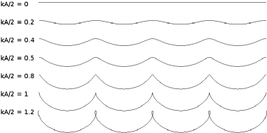
Figure 2: Shapes of waves obtained using Eq. 1

In order to obtain a realistic effect, the wave vector $\vec{k_{i}}$ of each wave is computed using scattering relationship in deep water domain, i.e. supposing that the bottom of the sea is located at infinite depth:

$$k_{i}=2\pi/\sqrt{\frac{gL_{i}}{2\pi}}$$ (2)

with $g$ the gravitation constant and $L_{i}$ the wavelength of each individual wave.

The same idea was developed with a simple bump mapping approach, where normal vectors on a planar mesh are transformed using a sum of $20$ cycloids [Sch80]. However, assuming that the bottom of the sea is at infinite depth limits the use of these methods since they don’t include more complex phenomena such as breaking waves or waves refraction near the shore. Peachey [Pea86] introduces a depth parameter to compute the wave vector $\vec{k_{i}}$ of each wave, using Airy wave theory:

$$k_{i}=2\pi/\sqrt{\frac{gL_{i}}{2\pi}tanh{\frac{2\pi d}{L_{i}}}}$$ (3)

where $d$ is the depth of a point related to the bottom of the sea.

Fournier and Reeves [FR86] suggested modifying Gerstner’s theory of waves, where water particles positions are given by:

$$\left\{\begin{array}[]{l}x=x_{0}-Ae^{ky_{0}}\sin(kx_{0}-wt)\\ y=y_{0}-Ae^{ky_{0}}\cos(kz_{0}-wt)\end{array}\right.$$ (6)

with $x$ (respectively $y$) the horizontal (resp. vertical) coordinate of a water particle at time $t$, $x_{0}$ and $y_{0}$ its coordinates at rest, $A$ the wave amplitude, $k$ the wave number and $w$ the wave pulsation. Fournier and Reeves enhance this model by taking into account the transformation of the path of water particles following the topological changes of the sea bed, and by transforming their circular path into a more realistic elliptic motion. This method permits to control the waves’ shape, more or less crested, through the use of different parameters, and therefore yields a more realistic result (see Figure 1).

Gonzato and Le Saec [GS99] modify this model when the starting point of a plunging breaking wave is detected near the shoreline (i.e. if the wave’s crest starts to curl over). This phenomenological modification results in the addition of two local functions applied to the wave’s shape: a stretch function imitates Biesel law by progressively stretching the wave along its crest, and a plunging function simulates gravity.

Ts’o and Barsky [TB87] suggested that the refraction of waves could be represented by the principle of light refraction formulated by Descartes. Their approach, called wave tracing, consists in generating a spline surface by casting rays from the skyline in a uniform 2D grid, progressing with Bresenham’s algorithm. The deviation of a ray is computed according to the depth difference of a cell to the next. However, a major drawback with this method is the lack of details on the generated surface when rays diverge significantly from a straight line, since in that case the number of rays defining the surface is too low. Gonzato and Le Saec [GS00] address this problem by generating new rays in undersampled areas, offering a better representation of the ocean surface around bays or islands for instance. This method called “Dynamic Wave Tracing” can handle wave reflexion and diffraction due to obstacles. This approach was also used by Gamito and Musgrave [GM02] to extract a phase map used in a parametric model, which can be animated easily. The height map representing the ocean surface can be rendered using enhanced ray tracing [GS00] or sphere tracing [DCG07] methods.

2.1.2 GPU implementations

Series of periodic functions are particularly well suited to GPU computations, and in the last few years research works describing real time implementations have emerged.

Chen et al [CLW07] use four sinusoids, computed in a vertex shader and transferred to a bump map in a pixel shader to simulate ripples. Salgado and Conci [SC07] describe a real-time implementation of Fournier’s method [FR86] using a vertex shader. Schneider and Westermann [SW01] compute a displacement map using Perlin noise in a vertex shader on the GPU to obtain interactive results. Isidoro et al [IVB02] use a precomputed mesh perturbed by four sinusoids with low frequencies in a vertex shader. Ripples are obtained by using a bump map combining multiple textures. When using a limited number of input functions, visually convincing surfaces are obtained in interactive time (see Figure 3). Cui et al [CYCXW04] follow the same approach combined with an adaptive tessellation of the surface using the method of Hinsinger et al [HNC02] (described in Section 2.3).

Chou and Fu [CF07] described a new GPU implementation for ocean simulation in order to take into account various interactions between the ocean surface and fixed or dynamic objects. The aim of this approach is to combine a particle system with a height-field obtained with a sum of sinusoids computed at each vertex of the surface mesh. Particles move according to the motion of each vertex but also to hydrodynamical forces [Bro91, FLS04] due to solid objects interacting in the scene.

2.1.3 Adaptive schemes

In order to limit computation time, adaptive schemes have been proposed to limit computations only in visible areas and/or to reduce the number of periodic functions used to represent the surface dynamically, depending on the distance to the viewer. This approach consists in discarding high frequencies in distant areas, also limiting aliasing effects such as moiré patterns visible on the horizon. The “grid project” concept proposed by Johanson [Joh04] consists in projecting the pyramid of vision onto the height map representing the water surface. Distant areas are automatically sampled at low resolution, whereas high resolution is used near the viewer.

Finch [Fin04] and Lee et al [LGL06a, LGL06b] propose a Level of Details (LOD) tessellation by adapting the resolution of the surface to the distance between the viewer and the horizontal plane; using the angle between the camera and the surface, vertices outside the pyramid of vision are also discarded before rendering stage. The implementation by Lee et al provides a $40\%$ gain in computation time compared to a fixed-resolution approach, and outperforms the implementation of Johanson [Joh04] (tests were conducted on a Pentium 4 at 3.0GHz and a GeForce 6600 GPU).

Kryachko [Kry05] use vertex textures, by computing two height maps representing the global motion of waves and fine scale details. The resolution is based on the distance to the viewer, allowing for fine-tune computations (see Figure 3).

Figure 3: Real-time ocean simulation from [Kry05]

2.2 Fourier domain approaches

This type of representation consists in describing the ocean surface using a spectral distribution of waves, obtained from theoretical or measured data. The spatial representation is then computed using the most significant frequency components and an inverse fast Fourier transform (IFFT), giving a geometric characterization of the surface as a dynamic height map defined for each point $X$ by:

$$h(X,t)=\sum_{i=1}^{N_{s}}\tilde{h}(\vec{k},t)e^{i\vec{k}X}$$ (7)

where $N_{s}$ is the number of spectral components, $\vec{k}$ is the wave vector and $\tilde{h}(\vec{k},t)$ is the amplitude of the Fourier component obtained from a theoretic wave spectrum.

2.2.1 General methods

This idea was proposed by Mastin et al [MWM87] with the Pierson-Moskowitz spectrum [PM64]. The amplitude of each Fourier component at time $t=0$ is given by:

$$\tilde{h_{0}}(\vec{k})=\frac{\alpha g^{2}}{16\pi^{4}f^{5}}e^{-\frac{5}{4}(\frac{f_{m}}{f})^{4}}$$ (8)

where $\alpha=0.0081$ is called Phillips’ constant, $g$ is the gravitation constant. The frequency peak $f_{m}$ is defined by:

$$f_{m}=\frac{0.13g}{U_{10}}$$ (9)

with $U_{10}$ the wind speed measured at $10$ meters above the surface.

Premoze and Ashikhmin [PA00] follow the same idea by using the JONSWAP spectrum [HBB^∗73], a modified version of Pierson-Moskowitz’s which reduces frequencies and thus raises waves’ amplitudes. The amplitude of each Fourier component at time $t=0$ in that case is slightly different:

$$\tilde{h_{0}}(\vec{k})=\frac{\alpha g^{2}}{16\pi^{4}f^{5}}e^{-\frac{5}{4}(\frac{f_{m}}{f})^{4}}e^{\ln(\gamma)e^{\frac{-(f-f_{m})^{2}}{2\sigma^{2}f_{m}^{2}}}}$$ (10)

with:

$$\sigma= \left\{\begin{array}[]{l}0.07\mbox{ if }f\leqslant f_{m}\\ 0.09\mbox{ if }f>f_{m}\end{array}\right.$$

The method presented by Tessendorf [Tes01] was notably used in famous computer-generated scenes for Waterworld and Titanic productions. Again, this approach uses spectral components to describe the surface, computed by a Gaussian pseudo-random generator and a theoretic wave spectrum due to Phillips:

$$\tilde{h_{0}}(\vec{k})=\frac{1}{\sqrt{2}}(\gamma_{r}+i\gamma_{i})\sqrt{P_{h}(\vec{k})}$$ (12)

with $\gamma_{r}$ and $\gamma_{i}$ defined as constants. The spectrum $P_{h}(\vec{k})$ is given by:

$$P_{h}(\vec{k})=C\frac{e^{-1/(kL)^{2}}}{k^{4}}|\vec{k}.\vec{w}|^{2}$$ (13)

where $C$ is a constant, $\vec{k}$ is the wave vector, $k$ is the wave number, $\vec{w}$ is the wind direction, $V$ is its speed and $L=\frac{V^{2}}{g}$. The choice of a random generator is justified by the Gaussian distribution of waves often observed in deep sea areas. In order to obtain fine details on the surface, each component is slightly perturbed by a noise function, producing more or less crested waves at any resolution (see Figure 4). Cieutat et al [CGG03] enhance this model in order to take in account water waves forces applied to a ship, implemented in a ship training simulator.

Although results obtained with this approach seem visually convincing for a distant viewer, when zooming towards the surface, waves’ shapes tend to look unrealistic since the resolution of the heightmap is fixed. In that case it becomes necessary to generate a new surface using more spectral components. This problem is addressed by interactive methods proposed recently.

2.2.2 Level-Of-Detail and GPU implementations

Hu et al [HVT^∗06] apply a LOD approach to Tessendorf’s method by representing the ocean with two surfaces. The first one, with a high, fixed resolution, is animated using a displacement map stored in a vertex shader, while the second one is sampled adaptively and applied as a bump map stored in a pixel shader. This approach produces a large ocean surface in real-time by animating only visible parts (at approx. $100$ frames/sec. on GeForce 3 GPU card). Mitchell [Mit05] implemented Tessendorf’s method on GPU by only considering frequencies generating a significant perturbation of the surface. A white noise is first generated using Phillips’ spectrum, then frequencies are divided in two sets. Low frequencies accounting for the global motion of waves are stored as a displacement map in a vertex shader. High frequencies, representing fine details, are stored in a normal map used for rendering. Since only a part of the spectrum is animated, a realistic ocean surface is obtained at interactive rates; another implementation by Chiu and Chang [CC06] combine this approach with an adaptive tessellation method [Joh04] (see previous section).

An adaptive spectrum sampling is presented by Frechot [Fre06] in order to obtain a more realistic surface with capillary waves or riddles. The main idea of this approach is to re-sample the spectrum corresponding to high frequencies areas, depending on the distance to the viewer. Robine and Frechot [RF06] also described a real-time additive sound synthesis method applied to the ocean surface. Sound synthesis methods are commonly used to efficiently sum a large number of sinusoidal components called partials. Here, ocean waves are considered as partials by shifting from the frequency and time domains to the wave number and spatial ones.

Figure 4: Ocean surface obtained in [Tes01]

2.3 Hybrid approaches

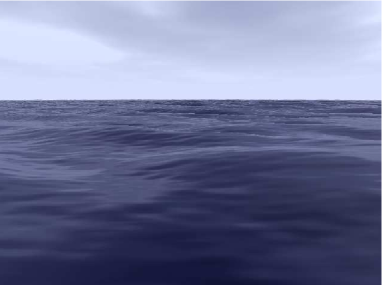
Figure 5: Ocean surface obtained in [TDG00]

Hybrid approaches are a combination of spatial and spectral definitions, generating a geometric representation of the surface while describing the components of wave trains in a realistic manner.

The method proposed by Thon et al [TDG00, TG02] shows a combination of a linear superposition of trochoids, which characteristics are synthesized using Pierson and Moskowitz’s spectrum. In order to get fine scale details, a 3D turbulence function is added to the surface; this method provides very realistic results, as shown on Figure 5.

Lee et al. [LBR07] combine a superposition of sinusoids and the TMA spectrum (Texel, Marson and Arsole, based on Jonswap’s) [BGRV85], creating a better statistical distribution of waves. It also offers better control for the end-user who can change parameters such as the bottom depth, thus enabling him to generate different types of water volumes (lakes, rivers, etc).

Xin et al [XFS06] extend the method of [TG02] to simulate the effects of wind variations over the surface by modulating each spectrum frequency accordingly.

Hinsingert et al [HNC02] apply a LOD scheme to the method of [TDG00] by reducing both the sampling resolution of the surface mesh and the number of trochoidal components depending on the distance to the viewer. This approach reduces the amount of computations for the ocean simulation and tends towards real-time rates (approximately $20$ to $30$ frames per sec. on a GeForce 2 GPU), by using only a subset of the components.

A real-time simulation method for ocean scenes was proposed by Lachman [Lac07] with a framework representing the surface either in the spatial domain by combining a spectrum and a sum of sinusoids or by using the approach of [Tes01]. This method is highly controllable, allowing the user to modify parameters such as the bottom depth or the agitation of the sea (defined by the Beaufort Scale). A LOD representation of the surface is also implemented to reduce computation costs. The main idea consists in defining several resolution levels from the projection of the pyramid of vision on the surface, and meshing the surface accordingly.

2.4 Discussion

		Model		Implementation
		Spatial	Spectral	Wave refraction	GPU	Level-Of-Details
1980	Schachter [Sch80]	x
1981	Max [Max81]	x
1986	Fournier et al. [FR86]	x
1987	Mastin et al. [MWM87]		x
1987	Ts’o et al. [TB87]	x		x
1999	Gonzato et al. [GS99]	x
2000	Gonzato et al. [GS00]	x		x
2000	Thon et al. [TDG00]	x	x
2001	Premoze et al. [PA00]		x
2001	Tessendorf [Tes01]		x
2001	Schneider et al. [SW01]	x			x
2002	Gamito et al. [GM02]	x		x
2002	Hinsinger et al. [HNC02]	x	x		x	x
2002	Isidoro et al. [IVB02]	x			x
2002	Thon et al. [TG02]	x	x
2003	Cieutat et al. [CGG03]		x	x
2004	Finch [Fin04]	x			x	x
2004	Johanson [Joh04]	x			x	x
2005	Kryachko [Kry05]	x			x	x
2005	Mitchell [Mit05]		x		x
2006	Chiu et al. [CC06]		x		x	x
2006	Frechot [Fre06]		x		x	x
2006	Hu et al. [HVT∗06]		x		x	x
2006	Lee et al. [LGL06a]	x			x	x
2006	Lee et al. [LGL06b]	x			x	x
2006	Robine et al. [RF06]		x		x
2006	Xin et al. [XFS06]	x	x		x	x
2007	Chen et al. [CLW07]	x			x
2007	Chou et al. [CF07]	x		x	x
2007	Lachman [Lac07]	x	x		x	x
2007	Lee et al. [LBR07]	x	x		x
2007	Salgado et al. [SC07]	x			x

Table 1: Classification of the simulation methods for deep water presented in section 2

The main advantage of spatial domain approaches is their ability to produce a simple and fast simulation of the ocean surface, but they require a large number of periodical functions for visually plausible results. Several optimizations have been proposed such as GPU evaluation or adaptive schemes to reduce this number according to the distance to the viewer. However, using sine or cosine functions induces a too rounded shape of waves and the surface appears too smooth.
Spectral domain methods address this problem by using oceanographic data directly and allow to disturb the surface according to physical parameters such as wind speed, which brings more realistic results. Unfortunately these methods lack from global control of ocean waves.
In this context, hybrid approaches represent a good compromise between the visually plausible results obtained by spectral approaches and the global control offered by spatial domain methods, and allow to obtain fast and effective simulations of the ocean surface’s dynamic behaviour. A complete summary of the methods presented in this section is shown on Table 1.

However, all these methods only consider deep water phenomena, in which the ocean surface is being subjected to small perturbations. Indeed, in shallow water parametric or spectral approaches cannot faithfully reproduce ocean dynamics near coasts, e.g. breaking waves. To address this complexity, we have to focus on approaches that consider interactions and collisions between the ocean and the shore, which are presented in the next section.

3 Ocean dynamics simulation in shallow water

Navier-Stokes equations (NSE) are able to capture the dynamic complexity of a fluid flow. Incompressible flow is usually considered for large volumes of fluid like oceans:

$$\nabla\vec{U}=0$$ (14)

$$\frac{\partial\vec{U}}{\partial t}+\vec{U}\nabla\vec{U}+\frac{\vec{\nabla}p}{\rho}-\mu\frac{\nabla^{2}\vec{U}}{\rho}-\vec{g}=0$$ (15)

with $\vec{U}=(u,v,w)$ the velocity of the fluid, $\mu$ its viscosity, $p$ its pressure, $\rho$ its density, and $\vec{g}$ representing gravity $(0,9.81,0)$. Operator $\nabla\vec{U}$ (resp. $\nabla^{2}\vec{U}$) is the gradient (resp. Laplacian) of $\vec{U}$ and is defined by $\nabla\vec{U}=(\frac{\partial u}{\partial t},\frac{\partial v}{\partial t},\frac{\partial w}{\partial t})$ (resp. $\nabla^{2}\vec{U}=\frac{\partial^{2}u}{\partial^{2}t}+\frac{\partial^{2}v}{\partial^{2}t}+\frac{\partial^{2}w}{\partial^{2}t}$). The first equation guarantees mass conservation, i.e. the density of the fluid remains constant over time. The second one guarantees moment conservation: the acceleration $\frac{\partial\vec{U}}{\partial t}$ of the fluid is equal to the sum of the applied forces weighted by its density. Other formulations for fluid behavior include shallow water equations (or Saint-Venant equations), preferably used whenever the horizontal scale is greater than the vertical one.

There are two main ways of discretizing these equations. On the one hand, Eulerian approaches use a 2D or a 3D grid where the fluid goes from cell to cell. On the other hand, Lagrangian approaches are based on particles carrying the fluid, thus representing small fluid volumes. Hybrid techniques were also developed to combine these two techniques, adding small-scale details to Eulerian simulations such as bubbles or spray. An excellent tutorial on physically-based simulation of fluids for Computer Graphics is presented by Bridson et al [BMFG06]. Adabala and Manohar [AM02] proposed a survey of most physically-based fluid simulation techniques. Since numerous phenomena can be simulated by these methods (fire, smoke, lava, etc.) we will focus on liquids and more specifically on ocean waters.

3.1 Eulerian approaches

Kass and Miller [KM90] were the first to use a physically-based realistic approach to represent the ocean surface. This method consists in solving Saint-Venant equations in 2D in order to obtain a heightmap. This was later extended by Chen and Lobo [CL95] to solve NSE taking into account pressure effects, hence generating a more realistic surface modulation.

A full 3D resolution of NSE was introduced in the Computer Graphics community by Foster and Metaxas [FM96, FM97], inspired from a physical approach proposed by Harlow and Welch [HW65] based on a uniform voxel decomposition of the 3D space. Velocity of the fluid is defined at the centers of each face of voxels; gradient and Laplacian are computed using finite differences between faces of adjacent voxels. Divergence at a given voxel is obtained from the updated velocities at its faces. In order to guarantee fluid incompressibility, the pressure field at a given voxel is modified according to the divergence. Virtual particles are placed in the voxel grid to extract the fluid surface, i.e. to discover its location, however the resulting surface does not look visually convincing. This problem was later addressed by Foster and Fedkiw [FF01] who represent it as an implicit, level-set surface evolving according to the fluid’s velocity. Nevertheless, visual results show compressibility artifacts since a noticeable volume of fluid disappears during the animation.

In order to solve this problem, Enright et al [EMF02] place particles above and below the surface, and advect them according to the velocity of the voxel they belong to. The surface is then computed by interpolating between the two implicit functions obtained from the locations of these particles. Since this approach called particles level-set method can be applied to all types of fluids, it became very popular and was widely used for many purposes, including the simulation of interactions between fluids and solids [CMT04, WMT05] or between different types of fluids [LSSF06]. The main drawback is high computational costs, which can be reduced by using an adaptive, octree-like structure [LGF04] to refine the voxel grid only near the fluid-solid or fluid-fluid interface.

This approach permits to capture the dynamic behavior of fluid surfaces in a realistic way and can be used for oceanic scenes. Enright et al [EMF02] simulate breaking waves by constraining the velocities in the grid using parametric equations [RO98]. Although realistic results are obtained, this approach can only handle limited types of waves (spilling or rolling waves). Mihalef et al [MMS04] simulate breaking waves by constraining velocities inside the grid using the parametric approach of Thon et al [TDG00] in 2D. The initial horizontal and vertical velocities of each element of fluid are given by:

$$\left\{\begin{array}[]{l}u=Awe^{k_{z}}\cos(k_{x})\\ v=Awe^{k_{z}}\sin(k_{x})\\ \end{array}\right.$$

where, as in [TDG00], $A$ is the amplitude of a wave, $\vec{k}=(k_{{x}},k_{{z}})$ its characteristic vector and $w$ its pulsation. The user can obtain any type of shore-break by choosing from a library of precomputed profiles. The full 3D simulation is then computed by extruding the desired profile along the parallel direction to the shore (see Figure 6).

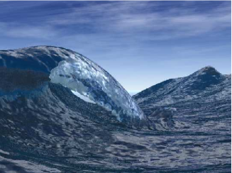
Figure 6: Eulerian breaking waves simulation from [MMS04]

Thürey et al [TMFSG07] simulate breaking waves in real-time, by solving Saint-Venant equations in 2D. A breaking wave is obtained by detecting regions with high curvatures on the heightmap representing the fluid, and adding a new mesh to account for the water falling from the crest. Each vertex of this mesh is projected in the 2D grid and advected using the corresponding cell.

3.2 Lagrangian approaches

In Lagrangian approaches, the fluid is represented by a set of particles following physical laws. Particle systems were first introduced in the computer graphics community by Reeves [Ree83] to simulate natural phenomena such as water, fire, clouds or smoke. Miller and Pearce [MP89] simulate interactions between particles by connecting them with the aid of springs to represent attraction or repulsion forces between neighboring particles, hence simulating viscous liquid flows. Terzopoulos et al [TPF89] later extended this method to simulate morphing from a solid to a liquid by modifying the stiffness of each spring. Tonnesen [Ton91] simulates the same kind of effects by solving heat transfer equations on the particles set.

Although realistic results are obtained with these methods, they are unable to simulate the inner dynamic complexity of fluids described by NSE. Stam and Fiume [SF95] introduced the Smoothed Particle Hydrodynamics (SPH) model in computer graphics, originally used in astrophysics to study the dynamics of celestial objects as well as their interactions [Luc77], and formalized by Monaghan [Mon92] for fluids. In that case, NSE are simplified and linearized. By considering that each particle has its own mass and that their sum gives the overall mass of the fluid, Equation 14 can be omitted since the overall mass remains constant over time. In equation 15, the non-linear advection term, representing the fluid’s transport related to its velocity in the Eulerian case, can be omitted: the fluid is transported by the particles themselves. Finally only one linear equation is necessary to describe the fluid’s velocity $\vec{U}$:

$$\frac{\partial{\vec{U}}}{\partial{t}}=\frac{1}{\rho}(-\nabla p+\mu\nabla^{2}\vec{U}+\rho g)$$ (17)

Let $\vec{f}=-\nabla p+\mu\nabla^{2}\vec{U}+\rho G$ represent the total amount of forces applied on a particle. The term $\nabla p$ accounts for pressure forces, $\mu\nabla^{2}\vec{U}$ for viscosity forces, and $\rho G$ for exterior forces. The acceleration $a$ of a particle is then given by:

$$a=\frac{\partial{\vec{U}}}{\partial{t}}=\frac{1}{\rho}(\vec{f}^{press}+\vec{f}^{visc}+\vec{f}^{ext})$$ (18)

where $\vec{f}^{press}$ (resp. $\vec{f}^{visc}$ and $\vec{f}^{ext}$) represents pressure (resp. viscosity and exterior forces). The main idea in the SPH approach consists in defining particles as potential implicit surfaces (also known as blobs or metaballs) influencing their neighbors. A particle represents an estimation of the fluid in a given region rather than a single molecule. Force computations rely on the interpolation of any scalar value $S_{i}$ for a given particle $i$, depending on its neighbors:

$$S_{i}=\sum_{j=1}^{N_{p}}m_{j}\frac{S_{j}}{\rho_{j}}W(r,R)$$ (19)

where $N_{p}$ is the total number of particles, $m_{j}$ (resp. $S_{j}$) is the mass (resp. the scalar value) of particle $j$, $r$ is the distance between particles $i$ and $j$, $R$ is the maximal interaction radius, and $W$ is a symmetric interpolation function. The gradient $\nabla S_{i}$ and Laplacian $\nabla^{2}S_{i}$ are given by:

$$\nabla S_{i}=\sum_{j=1}^{N}m_{j}\frac{S_{j}}{\rho_{j}}\nabla W(r,R)$$ (20)

$$\nabla^{2}S_{i}=\sum_{j=1}^{N}m_{j}\frac{S_{j}}{\rho_{j}}\nabla^{2}W(r,R)$$ (21)

Equation 19 can then be used to compute the density of a particle $i$; pressure and viscosity computation will rely on equations 20 and 21.

The SPH model was extended by several authors [DC96, SAC^∗99] to represent elastic deformations, lava flows, etc. by simulating heat transfer and varying viscosity. Müller et al [MCG03] presented an extension to simulate low compressible liquids such as water. Clavet et al [CBP05] represent visco-elastic fluids by coupling particles with a mass-spring system; particles advection is governed by Navier-Stokes equations but also Newtonian spring dynamics, which slows the fluid down depending on springs stiffness. Another extension by Müller et al [MSKG05] represent interactions between fluids with different phases by modifying the viscosity between neighboring particles. This method can also simulate bubbles generated by heating, using varying densities for fluid particles to represent the amount of gasification.

However, two problems are inherent to the SPH approach. First of all, compressibility effects can be observed when the volume does not remain constant over time, yielding non-realistic visualizations. Besides, a huge amount of particles is needed to simulate large volumes of water with fine-scale details, leading to high computation and memory consumption. These problems were addressed by several authors.

Premoze et al [PTB^∗03] introduced the Moving Particle Semi-implicit method (MPS) in computer graphics from physically-based models [KO96, YKO96]. This approach is an extension of SPH where the density of a particle is modified to guarantee constant pressure through the solving of a Poisson equation. It was extended by Wang et al [WZC^∗06] to simulate 2D breaking waves, combined to obtain a 3D surface. Becker and Teschner [BT07] guarantee near-incompressibility by modifying pressure depending on density variations. Since pressure is directly related to attraction or repulsion forces between particles, it is possible to ensure a near constant distance between neighboring particles, hence a near constant volume. An alternative method was also presented more recently by Solenthaler and Pajarola [SP09].

Adaptive schemes were proposed to reduce the number of particles and limit computation and memory costs for simulating large volumes of fluid. Desbrun and Cani [DC99] merge or split particles according to their density. The overall mass of the system is kept constant by re-computing particle masses as soon as they are subjected to one of these operations. In order to guarantee symmetric interactions between particles with different masses, a shooting / gathering scheme ensures that attraction or repulsion forces are equal. Although this approach reduces computation costs, visual artifacts can be observed during animations because of instantaneous merging or splitting of particles near the surface. The adaptive scheme proposed by Hong et al [HHK08] consists in varying the size and number of particles according to their position relative to a fixed set of layers defined by the user in a preprocessing step. Finally, Adams et al [APKG07] obtain adaptively sized particles by defining merging or splitting processes, depending on the distance to the viewer or to the surface. This ensures that visual artifacts are avoided near the surface since only particles deep inside the fluid can be modified. This approach was implemented on GPU by Yan et al [YWH^∗09] to simulate breaking waves in real-time.

3.3 Hybrid approaches

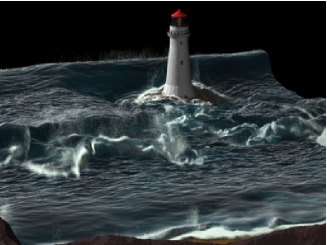
Figure 7: Hybrid simulation from [LTKF08]

The main idea in hybrid approaches is to simulate the main body of fluid using an Eulerian method, and fine-scale details such as foam, spray or bubbles with a Lagrangian method. By adding small details, very realistic results are obtained, and interest for this approach is growing more and more with the development of efficient simulations. O’Brien and Hodgins [OH95] couple an Eulerian method with a particle system to represent sprays. Navier-Stokes equations are solved in 2D, and sprays are generated depending on the magnitude of the vertical velocity at each cell; these particles are then advected using the velocity in the grid. The Eulerian simulation of Takahashi et al [TFK^∗03] is coupled with particles generated in high curvature regions, then advected independently. Greenwood and House [GH04] use a level-set approach [EMF02] coupled with particles generated in high curvature regions, advected using the velocity of their corresponding cell. The friction of the fluid is also taken into account to generate bubbles.This method was later extended by Zheng et al [ZYP06] by deforming each bubble based on surface tension, thus avoiding non-realistic spherical bubbles.

Kim et al [KCC^∗06] extend an adaptive level-set approach [LGF04] to generate particles according to the temporal variation of the volume of fluid in each cell. The main idea consists in using particles advected below the surface, transformed into water or air at the rendering stage. Since the number of transformed particles depends on the volume of water lost in a cell, this characterizes the turbulence in that cell and hence generates particles in highly perturbed regions.

Yuksel et. al [YHK07] introduced the concept of wave particles to simulate waves and their interactions with solid objects. Wave particles are defined by a disturbance function characterized by an amplitude, a propagation angle and a maximal interaction distance. The fluid itself is represented by a height-field whose values are computed according to neighbouring wave particles. When waves collide with solid objects, propagation angles are re-computed according to the curvature at collision points and new particles are generated to obtain waves refraction.

Thürey et al [TRS06] proposed to couple 2D and 3D simulations using Saint-Venant equations solved with a Lattice-Boltzmann method [FDH^∗87]. The 2D simulation accounts for global motion of the surface, but fine-scale details are represented in 3D. These two layers interact with each other to generate foam and sprays, by creating particles according to the velocity in each cell and surface tension at the air-water interface. This work was later extended with SPH to represent interactions between particles in [TSS^∗07]. The same approach is followed by Losasso et al [LTKF08] to combine an Eulerian method with SPH particles whose number is computed from the divergence of the fluid’s velocity, thus simulating bubbles or sprays generated by breaking waves (see Figure 7).

3.4 Discussion

		Model		Resolution		Implementation
		Eulerian	Lagrangian	2D-based	Full 3D	Incompressibility	LOD
1989	Miller et al. [MP89]		x		x
1989	Terzopoulos et al. [TPF89]		x		x
1990	Kass et al. [KM90]	x		x
1991	Tonnesen [Ton91]		x		x
1995	Stam et al. [SF95]		x		x
1995	Chen et al. [CL95]	x		x
1995	O’Brien et al. [OH95]	x	x	x
1996	Desbrun et al. [DC96]		x		x
1996	Foster et al. [FM96]	x			x
1997	Foster et al. [FM97]	x			x
1999	Desbrun et al. [DC99]		x		x		x
1999	Stora et al. [SAC∗99]		x		x
2001	Foster et al. [FF01]	x			x
2002	Enright et al. [EMF02]	x			x	x
2003	Premoze et al. [PTB∗03]		x		x	x
2003	Muller et al. [MCG03]		x		x
2003	Takahashi et al. [TFK∗03]	x	x		x	x
2004	Carlson et al. [CMT04]	x			x	x
2004	Greenwood et al. [GH04]	x	x		x
2004	Losasso et al. [LGF04]	x			x	x	x
2004	Mihalef et al. [MMS04]	x		x		x
2005	Clavet et al. [CBP05]		x		x
2005	Muller et al. [MSKG05]		x		x
2005	Wang et al. [WMT05]	x			x	x
2006	Kim et al. [KCC∗06]	x	x		x		x
2006	Losasso et al. [LSSF06]	x			x	x
2006	Thurey et al. [TRS06]	x	x	x	x	x
2006	Wang et al. [WZC∗06]		x	x	x	x
2006	Zheng et al. [ZYP06]	x	x		x	x
2007	Adams et al. [APKG07]		x		x		x
2007	Becker et al. [BT07]		x		x	x
2007	Thurey et al. [TMFSG07]	x		x	x
2007	Thurey et al. [TSS∗07]	x	x	x		x
2007	Yuksel et al. [YHK07]	x	x	x	x
2008	Hong et al. [HHK08]		x		x		x
2008	Losasso et al. [LTKF08]	x	x		x	x
2009	Solenthaler et al. [SP09]		x		x	x
2009	Yan et al. [YWH∗09]		x		x		x

Table 2: Classification of the simulation methods for shallow water presented in section 3

The main advantage of Eulerian approaches is their ability to simulate a large scope of different phenomena, explaining why they received much attention from the computer graphics community. Nevertheless, for fine-scale details such as spray or bubbles, NSE need to be finely discretized which in turn demands high computations and memory consumption. Another drawback is the use of fixed grids, forbidding the fluid to flow outside the grid.

On the other hand, Lagrangian approaches can be used to simulate a wide range of phenomena. Their main advantage is their ability to represent fine-scale details and to flow anywhere in a virtual environment, but a large number of particles is usually needed to obtain realistic results. This problem can be alleviated using adaptive split-and-merge schemes to reduce computation costs. However it is worth noticing that most of the computation time for one particle is spent in testing neighboring particles or other objects for collision. Therefore a broad-phase collision detection is usually implemented by storing particles in a virtual grid, meaning that Eulerian or Lagrangian approaches share common problems such as defining an appropriate size for the grid’s cells. This is also illustrated by hybrid methods which produce realistic results by adding details to Eulerian approaches using particle systems. The literature presented in section 3 is summarized on Table 2.

4 Realistic ocean surface rendering and lighting

In the previous sections we presented different approaches to obtain a plausible shape of the ocean surface, in deep water or near the shoreline. This surface can then be rendered using water shaders implementing light reflection and refraction described by Fresnel equations. Nevertheless, the ocean’s visual aspect is characterized by numerous interactions. Their impact is visible through several phenomena such as foam, sprays and light interactions, addressed by several methods in computer graphics. Some of them were already mentioned earlier, when the fluid simulation algorithm includes these phenomena directly (e.g. bubbles), However in most cases rendering is performed in a post-processing step. We focus on the following on different methods designed to enhance the realism of ocean scenes.

4.1 Foam and spray

Foam and spray rendering methods can be divided into two types: on the one hand, methods based on the computation of foam amount at one point on the ocean according to empirical models, and on the other hand, methods based on particle systems and rendered as point clouds.

4.1.1 Empirical models

Jensen and Golias [JG01] compute the amount of foam at a given point according to its height: if the height difference with its neighbors is greater than a predefined threshold, foam is generated and rendered using a semi-transparent texture (see Figure 8). This method was extended by Jeschke et al [JBS03] to take into account the amplitude of ocean waves. The main drawback with this approach is encountered when trying to animate foam, since its motion does not follow the waves. Another problem arises from the empirical models that do not consider atmospheric conditions which are, in reality, the main cause of the apparition of foam. Oceanographic observations have shown for example that foam only appears when wind velocity exceeds $13$km/h [Mun47].

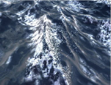
Figure 8: Foam rendering from [JG01]

Premoze and Ashikhmin [PA00] compute the amount of foam based on wind velocity and the temperature difference between water and air. The user can control atmospheric conditions to induce more or less foam. However, results are limited by several constraints on the surface, and the animation is not visually convincing. Darles et al [DCG07] extend this method with an animated texture, combined with other phenomena such as light attenuation due to spray particles in the air.

4.1.2 Particle systems

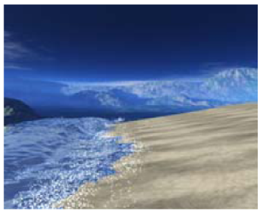
Figure 9: Spray rendering from [WZC^∗06]

Peachey [Pea86] first proposed to use particle systems in order to represent spray generated by breaking waves. Wang et al [WZC^∗06] extend this approach by describing breaking waves using a Lagrangian approach, and generating spray subsystems according to the velocity of water particles (see Figure 9). Holmberg and Wunsche [HW04] generate foam particles by considering the amplitude of the waves, and render them as cloud points. The same idea is used by other authors [JG01, JBS03, CC06] to generate spray particles according to the temporal variation of height at a given point. Although these methods provide realistic results, they also demand high computations since a large number of particles is needed; this proves difficult to handle when rendering large oceanic scenes.

4.2 Light-water interactions

Light-water interactions play an important role in the way we perceive ocean’s color, however they must be approximated especially for real-time implementations. We use their order of approximation to classify existing methods, from strong simplifications of optics laws to highly accurate computations generating rippling caustics formed when light shines through ocean waves.

4.2.1 First order approximation

A first approach consists in rendering light-water interaction by applying geometrical optics laws, using Fresnel coefficients or Schlick’s approximation [Sch94]. The Beer-Lambert law reduces the intensity $I$ of a light ray by an exponential factor, depending on the covered distance $d$ (i.e. the distance traveled by the ray from the light source to the intersection point) and an attenuation coefficient $a$:

$$I=I(0)e^{-ad}$$ (22)

where $I(0)$ is the initial intensity of the ray. In the case of reflexion, intensity can be reduced according to the optical depth due to particles in the air. For refraction, the reduction comes from the attenuation coefficient of water, as implemented by Tessendorf [Tes01].

Gonzato and Le Saec [GS00] use Ivanoff’s table defining the color of an ocean depending on its position on Earth [JN74]. This color takes into account reflected and refracted light, and in presence of submarine objects, a fast light absorption method is applied by using an ocean water absorption spectrum.

In order to reduce computation costs and obtain realistic results in real-time, simpler methods and GPU implementations are often preferred. An environment mapping method can be enough to approximate reflexion and refraction effects. In both cases, the viewer is assumed to be far from the considered point, thus incident rays are considered parallels and reflected rays only depend on the surface’s normal vector. This technique is commonly used in computer graphics, especially for ocean surface rendering [SW01, JG01]. Baboud and Decoret [BD06] represent refraction by an environment map of the bottom of the sea. An alternative method was proposed by different authors [Bel03, HVT^∗06] by mapping a sky texture onto the surface and considering this surface as perfectly specular.

Recently Bruneton et al. [BNH10] proposed a GPU implementation of ocean lighting based on a hierarchical representation mixing geometry, normals and BRDF. The reflected light coming from the sun and the sky and the light refracted by the ocean are simulated by combining the BRDF model of Ross et al. [VRP05] and wave slope variance (i.e. normals) depending on the required level of detail.

4.2.2 Multiple order approximation

When a light ray enters the ocean surface, a fraction is diffused, absorbed and reflected on organic particles in suspension near the surface. In order to represent the complexity of this phenomenon and compute the amount of light at any point inside the water volume, a Radiative Transfer equation (RTE) must be solved.

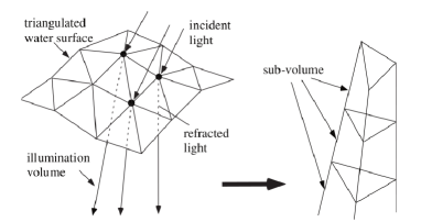
Figure 10: Creation of illumination volumes from [IDN02]

Arvo [Arv86] propose to emit rays from light sources and to accumulate them in illumination maps to represent caustics. Iwasaki et al [IDN01, IDN03] use beam-tracing methods [HH84, Wat90] to solve RTE by discretizing the water volume into illumination volumes formed by the intersection of refracted rays and the bottom of the sea, sliced into sub-volumes (see Figure 10). The amount of light bouncing back to the surface is computed by accumulating light in all traversed sub-volumes. By discretizing the water volume into horizontal, planar sheets, bouncing light can be computed by accumulating light at intersection points between rays and each sheet to obtain caustics. The photon mapping method proposed by Jensen [Jen01] can also simulate caustics or other global illumination effects.

Nishita et al [NSTN93] proposed a rendering algorithm to visualize oceans viewed from space by taking into account optical properties due to atmospheric conditions. The color of the ocean is computed using a spectral model based on the RTE which takes several physicals parameters into account such as ocean depth, incident angles of the sun and viewing direction.

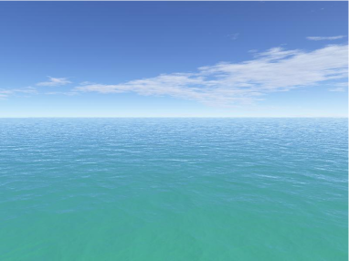
Figure 11: Ocean surface rendering for a clear water from [PA00]

Sub-surface scattering was also addressed by several authors [PA00, CS04] by taking into account several bio-optical parameters such as chlorophyll concentration and turbidity [Jer76]. In that case, coefficients for attenuation $a(\lambda)$ and diffusion $b(\lambda)$ are obtained from physical laws [Mor91, GM83] according to the phytoplankton concentration $C_{p}$ inside water:

$$a(\lambda)= (a_{w}(\lambda)+0.06C_{p}^{0.65})(1+0.02e^{-0.014(\lambda-380)})$$

$$b(\lambda)= \frac{550}{\lambda}0.30C_{p}^{0.32}$$

where $a_{w}(\lambda)$ is the attenuation coefficient of pure water for a given wavelength $\lambda$. Thus turbidity is directly related to the concentration of phytoplankton. This approach is able to represent realistic ocean colors according to their biological properties (see Figure 11).

Gutierrez et al [GSAM08] simulate a wider range of phenomena such as inelastic diffusion of light rays, fluorescence effects due to phytoplankton particles and Raman diffusion, observed when an incident ray’s wavelength is modified because of water properties. This model is able to characterize the visual impact of different kinds of sediments on the resulting image, and thus represent different ocean waters depending on their bio-chemical composition.

Finally another type of methods consider subsurface scattering inside water as participating media. Interested readers should refer to [PCPS97] for an overview of these methods.

4.3 Discussion

Numerous methods are available in the literature to take different optical phenomena into account and increase the realism of oceanic scenes. In the case of foam and sprays, empirical methods can effectively simulate these phenomena according to the state of disturbance of the surface. Combined with particle systems, these approaches allow to obtain realistic details, however they require a large number of particles which induces an important memory cost and computation time at rendering stage. Moreover, empirical methods are usually efficient for deep water scenes only; to our knowledge there is no work dealing with realistic foam created by breaking waves.
For light-water interactions, different methods were proposed to represent the complexity of these non-linear phenomena, yielding more and more realistic results. Moreover, recent approaches even consider physical and biology effects to simulate a wide variety of virtual environments. All these works are summarized on Table 3.

		Foam and Spray		Light-water interactions
		Empirical	Particles	First order	Multiple order
1986	Arvo [Arv86]				x
1986	Peachey [Pea86]		x
1993	Nishita et al. [NSTN93]			x
2000	Gonzato et al. [GS00]			x
2000	Premoze et al. [PA00]	x			x
2001	Iwasaki et al. [IDN01]				x
2001	Jensen [Jen01]				x
2001	Jensen et al. [JG01]	x	x	x
2001	Schneider et al. [SW01]			x
2001	Tessendorf [Tes01]			x
2003	Belyaev [Bel03]			x
2003	Iwasaki et al. [IDN03]				x
2003	Jeschke et al. [JBS03]	x	x
2004	Cerezo et al. [CS04]				x
2004	Holmberg et al. [HW04]		x
2006	Chiu et al. [CC06]		x
2006	Baboud et al. [BD06]			x
2006	Hu et al. [HVT∗06]			x
2006	Wang et al. [WZC∗06]		x
2007	Darles et al. [DCG07]	x		x
2008	Gutierrez et al. [GSAM08]				x
2010	Bruneton et al. [BNH10]			x

Table 3: Classification of the realistic rendering methods presented in section 4

5 Conclusion

In this survey we have presented available methods in computer graphics for modeling and rendering oceanic scenes. The great amount of different works is inherent to the extreme diversity of the phenomena involved.

The first two sections of our survey focused on computer graphics models able to simulate the dynamical behavior of the ocean. We have seen that those methods are divided into two categories: on the one hand, methods usually dedicated to deep-water simulation, on the other hand fluid-based approaches trying to represent breaking waves near the shore. In the last section, we have seen different methods able to represent several phenomena involved in ocean rendering, namely foam, sprays and light-water interactions, that make for visual realism.

The next decade could see new methods emerging in an attempt to bridge the gap between deep-sea simulations and breaking waves representations; it would be necessary to put together different types of simulations on different scales. Scalable methods are also required for modeling and rendering stages in order to obtain real-time rates, which could include dynamic sampling of the simulation domain (as proposed by Yu et al [YNBH09] for rivers) and adaptive rendering models taking the visual impact of the considered phenomena into account.

References

- [AM02] Adabala N., Manohar S.: Techniques for realistic visualization of fluids: A survey. Computer Graphics Forum 21, 1 (2002), 65–81.
- [APKG07] Adams B., Pauly M., Keiser R., Guibas L.: Adaptively sampled particle fluids. In ACM Transactions on Graphics (2007), vol. 26.
- [Arv86] Arvo J.: Backward ray tracing. In In ACM SIGGRAPH ’86 Course Notes - Developments in Ray Tracing (1986), pp. 259–263.
- [BD06] Baboud L., Décoret X.: Realistic water volumes in real-time. In Eurographics Workshop on Natural Phenomena (2006).
- [Bel03] Belyaev V.: Real-time simulation of water surface. In Graphicon (2003).
- [BGRV85] Bouws E., Günther H., Rosenthal W., Vincent C.: Similarity of the wind wave spectrum in finite depth water: Part 1. spectral form. Journal of Geophysical Research 90 (1985), 975–986.
- [Bie52] Biesel F.: Study of wave propagation in water of gradually varying depth. In Gravity Waves (1952), 243–253.
- [BMFG06] Bridson R., Müller-Fischer M., Guendelman E.: Fluid simulation. SIGGRAPH 2006 Course Notes (2006).
- [BNH10] Bruneton E., Neyret F., Holzschuch N.: Real-time realistic ocean lighting using seamless transitions from geometry to brdf. Computer Graphics Forum 29, 2 (2010).
- [Bro91] Browing A.: A mathematical model to simulate small boat behaviour. SIMULATION 56 (1991).
- [BT07] Becker M., Teschner M.: Weakly compressible sph for free surface flows. In SCA ’07: Proceedings of the 2007 ACM SIGGRAPH/Eurographics symposium on Computer animation (2007), pp. 209–217.
- [CBP05] Clavet S., Beaudoin P., Poulin P.: Particle-based viscoelastic fluid simulation. In SCA ’05: Proceedings of the 2005 ACM SIGGRAPH/Eurographics symposium on Computer animation (july 2005), pp. 219–228.
- [CC06] Chiu Y.-F., Chang C.-F.: Gpu-based ocean rendering. IEEE International Conference on Multimedia and Expo (2006), 2125–2128.
- [CF07] Chou C.-T., Fu L.-C.: Ships on real-time rendering dynamic ocean applied in 6-dof platform motion simulator. In CACS International Conference (2007).
- [CGG03] Cieutat J.-M., Gonzato J.-C., Guitton P.: A general ocean waves model for ship design. In Virtual Concept (2003).
- [CL95] Chen J., Lobo N.: Toward interactive-rate simulation of fluids with moving obstacles using navier-stokes equations. Graph. Models Image Process. 57, 2 (1995), 107–116.
- [CLW07] Chen H., Li Q., Wang G.: An efficient method for real-time ocean simulation. Technologies for E-Learning and Digital Entertainment 4469 (2007), 3–11.
- [CMT04] Carlson M., Mucha P., Turk G.: Rigid fluid: animating the interplay between rigid bodies and fluid. In ACM SIGGRAPH (2004), pp. 377–384.
- [CS04] Cerezo E., Seron F.: Rendering natural waters taking fluorescence into account. Comput. Animat. Virtual Worlds 15, 5 (2004), 471–484.
- [CYCXW04] Cui X., Yi-Cheng J., Xiu-Wen L.: Real-time ocean wave in multi-channel marine simulator. In International conference on Virtual Reality continuum and its applications in industry (2004), pp. 332–335.
- [DC96] Desbrun M., Cani M.-P.: Smoothed particles: A new paradigm for animating highly deformable bodies. In Eurographics Workshop on Computer Animation and Simulation (EGCAS) (1996), pp. 61–76.
- [DC99] Desbrun M., Cani M.-P.: Space-Time Adaptive Simulation of Highly Deformable Substances. Research report 3829, INRIA, 1999.
- [DCG07] Darles E., Crespin B., Ghazanfarpour D.: Accelerating and enhancing rendering of realistic ocean scenes. In WSCG (2007).
- [EMF02] Enright D., Marschner S., Fedkiw R.: Animation and rendering of complex water surfaces. ACM Transactions on Graphics 21, 3 (2002), 736–744.
- [FDH∗87] Frish U., D’Humières D., Hasslacher B., Lallemand P., Pomeau Y., Rivert J.-P.: Lattice gas hydrodynamics in two and three dimensions. Complex System 1 2 (1987), 649–707.
- [FF01] Foster N., Fedkiw R.: Practical animation of liquids. In ACM SIGGRAPH (2001), pp. 23–30.
- [Fin04] Finch M.: Effective water simulation from physical models. GPU Gems (2004), 5–29.
- [FLS04] Fang M., Lin K., Shu Z.: An indigenous pc-based ship simulator incorporating the hydrodynamic numerical model and virtual reality technique. Journal of the Society of Naval Architects and Marine Engineers 23 (2004), 87–95.
- [FM96] Foster N., Metaxas D.: Realistic animation of liquids. Graph. Models Image Process. 58, 5 (1996), 471–483.
- [FM97] Foster N., Metaxas D.: Controlling fluid animation. In Computer Graphics International (1997).
- [FR86] Fournier A., Reeves W.: A simple model of ocean waves. ACM SIGGRAPH (1986), 75–84.
- [Fre06] Frechot J.: Realistic simulation of ocean surface using wave spectra. In GRAPP (2006), pp. 76–83.
- [GH04] Greenwood S., House D.: Better with bubbles: enhancing the visual realism of simulated fluid. In SCA ’04: Proceedings of the 2004 ACM SIGGRAPH/Eurographics symposium on Computer animation (2004), pp. 287–296.
- [GM83] Gordon H., Morel A.: Remote assesment of ocean color for interpretation of satellite visible imagery, a review. Lecture Notes on Coastal and Estuarine Studies 4 (1983).
- [GM02] Gamito M., Musgrave F.: An acurrate model of wave refraction over shallow water. Computers & Graphics 26, 2 (2002), 291–307.
- [GS99] Gonzato J.-C., Saec B. L.: On modeling and rendering ocean scenes (diffraction, surface tracking and illumination). In WSCG (1999), pp. 93–101.
- [GS00] Gonzato J.-C., Saec B. L.: On modeling and rendering ocean scenes. Journal of Visualisation and Computer Simulation 11 (2000), 27–37.
- [GSAM08] Gutierrez D., Seron F., Anson O., Muñoz A.: Visualizing underwater ocean optics. Computer Graphics Forum 27, 2 (2008), 547–556.
- [HBB∗73] Hasselman K., Barnett T., Bouws E., Carlson D. E., Hasselmann P.: Measurements of wind-wave growth and swell decay during the joint north sea wave project (jonswap). Deutsche Hydrographische Zeitschrift A8, 12 (1973).
- [HH84] Heckbert P., Hanrahan P.: Beam tracing polygonal objects. In ACM SIGGRAPH (1984), pp. 119–127.
- [HHK08] Hong W., House D., Keyser J.: Adaptive particles for incompressible fluid simulation. The Visual Computer 24, 7 (2008), 535–543.
- [HNC02] Hinsinger D., Neyret F., Cani M.-P.: Interactive animation of ocean waves. In SCA ’02: Proceedings of the 2002 ACM SIGGRAPH/Eurographics symposium on Computer animation (2002), pp. 161–166.
- [HVT∗06] Hu Y., Velho L., Tong X., Guo B., Shum H.: Realistic, real-time rendering of ocean waves. Comput. Animat. Virtual Worlds 17, 1 (2006), 59–67.
- [HW65] Harlow F., Welch J.: Numerical calculation of time-dependent viscous incompressible flow of fluid with free surface. Phys. Fluids 8 (1965), 2182–2189.
- [HW04] Holmberg N., Wünsche B.: Efficient modeling and rendering of turbulent water over natural terrain. In GRAPHITE ’04: Proceedings of the 2nd international conference on Computer graphics and interactive techniques in Australasia and South East Asia (New York, NY, USA, 2004), ACM, pp. 15–22.
- [IDN01] Iwasaki K., Dobashi Y., Nishita T.: Efficient rendering of optical effects within water using graphics hardware. In PG ’01: Proceedings of the 9th Pacific Conference on Computer Graphics and Applications (2001), pp. 374–383.
- [IDN02] Iwasaki K., Dobashi Y., Nishita T.: An efficient method for rendering underwater optical effects using graphics hardware. Computer Graphics Forum 21, 4 (2002), 701–711.
- [IDN03] Iwasaki K., Dobashi Y., Nishita T.: A volume rendering approach for sea surfaces taking into account second order scattering using scattering maps. In Workshop on Volume graphics (2003), pp. 129–136.
- [Igl04] Iglesias A.: Computer graphics for water modeling and rendering: a survey. Future Generation Computer Systems 20, 8 (2004).
- [IVB02] Isidoro J., Vlachos A., Brennan C.: Rendering ocean water. Direct3D ShaderX : Vertex and Pixel Shader Tips and Tricks Wordware (2002).
- [JBS03] Jeschke S., Birkholz H., Shumann H.: A procedural model for interactive animation of breaking ocean waves. In WSCG (2003).
- [Jen01] Jensen H.: Realistic image synthesis using photon mapping. A. K. Peters, Ltd., Natick, MA, USA, 2001.
- [Jer76] Jerlov N.: Marine Optics. Elsevier, 1976.
- [JG01] Jensen L., Golias R.: Deep-water animation and rendering, 2001.
- [JN74] Jerlov N., Nielsen E.: Optical Aspects of Oceanography. Academic Press, 1974.
- [Joh04] Johanson C.: Real-Time water rendering - Introducing the projected grid concept. Master’s thesis, Lund University, 2004.
- [KCC∗06] Kim J., Cha D., Chang B., Koo B., Ihm I.: Practical animation of turbulent splashing water. In SCA ’06: Proceedings of the 2006 ACM SIGGRAPH/Eurographics symposium on Computer animation (2006), pp. 335–344.
- [KM90] Kass M., Miller G.: Rapid, stable fluid dynamics for computer graphics. In ACM SIGGRAPH (1990), pp. 49–57.
- [KO96] Koshizuka S., Oka Y.: Moving-particle semi-implicit method for fragmentation of incompressible fluid. Nuclear Science Engineering, 123 (1996), 421–434.
- [Kry05] Kryachko Y.: Using vertex texture displacement for realistic water rendering. GPU Gems 2 (2005), 283–294.
- [Lac07] Lachman L.: An open programming architecture for modeling ocean waves. In IMAGE Conference (2007).
- [LBR07] Lee N., Baek N., Ryu K.: Real-time simulation of surface gravity ocean waves based on the tma spectrum. In International conference on Computational Science (2007), pp. 122–129.
- [LGF04] Losasso F., Gibou F., Fedkiw R.: Simulating water and smoke with an octree data structure. In ACM SIGGRAPH (2004), pp. 457–462.
- [LGL06a] Lee H.-M., Go C., Lee W.-H.: An efficient algorithm for rendering large bodies of water. Entertainment Computing - ICEC 4161 (2006), 302–305.
- [LGL06b] Lee H.-M., Go C., Lee W.-H.: A frustrum-based ocean rendering algorithm. Agent Computing and Multi-Agent Systems 4088 (2006), 584–589.
- [LSSF06] Losasso F., Shinar T., Selle A., Fedkiw R.: Multiple interacting liquids. ACM Transactions on Graphics 25, 3 (2006), 812–819.
- [LTKF08] Losasso F., Talton J., Kwatra N., Fedkiw R.: Two-way coupled sph and particle level set fluid simulation. IEEE Transactions on Visualization and Computer Graphics 14, 4 (2008), 797–804.
- [Luc77] Lucy L. B.: A numerical approach to the testing of the fission hypothesis. Astron Journ. 82, 12 (December 1977), 1013–1924.
- [Max81] Max N.: Vectorized procedural models for natural terrain: Waves and islands in the sunset. In ACM SIGGRAPH (1981), pp. 317–324.
- [MCG03] Müller M., Charypar P., Gross M.: Particle-based fluid simulation for interactive applications. In SCA ’03: Proceedings of the 2003 ACM SIGGRAPH/Eurographics symposium on Computer animation (2003), pp. 154–159.
- [Mit05] Mitchell J.: Real-Time Synthesis and Rendering of Ocean Water. Tech. rep., ATI Research, 2005.
- [MMS04] Mihalef V., Metaxas D., Sussman M.: Animation and control of breaking waves. In SCA ’04: Proceedings of the 2004 ACM SIGGRAPH/Eurographics symposium on Computer animation (2004), pp. 315–324.
- [Mon92] Monaghan J.: Smoothed particle hydrodynamics. Ann. Rev. Astron. Astrophys. 30 (1992), 543–574.
- [Mor91] Morel A.: Light and marine photosynthesis : a spectral model with geochemical and climatological implications. Prog. Oceanogr. 63 (1991).
- [MP89] Miller G., Pearce A.: Globular dynamics: a connected particle system for animating viscous fluids. Computers & Graphics 13, 3 (1989), 305–309.
- [MSKG05] Müller M., Solenthaler B., Keiser R., Gross M.: Particle-based fluid-fluid interaction. In SCA ’05: Proceedings of the 2005 ACM SIGGRAPH/Eurographics symposium on Computer animation (2005), pp. 237–244.
- [Mun47] Munk W.: A critical wind speed for air-sea boundary processes. Journal of Marine Research 6 (1947), 203.
- [MWM87] Mastin G., Watterberg P., Mareda J.: Fourier synthesis of ocean scenes. IEEE Comput. Graph. Appl. 7, 3 (1987), 16–23.
- [NSTN93] Nishita T., Sirai T., Tadamura K., Nakamae E.: Display of the earth taking into account atmospheric scattering. In ACM SIGGRAPH (New York, NY, USA, 1993), ACM, pp. 175–182.
- [OH95] O’Brien J., Hodgins J.: Dynamic simulation of splashing fluids. In CA ’95: Proceedings of the Computer Animation (Washington, DC, USA, 1995), IEEE Computer Society, p. 198.
- [PA00] Premoze S., Ashikhmin M.: Rendering natural waters. In PG ’00: Proceedings of the 8th Pacific Conference on Computer Graphics and Applications (Washington, DC, USA, 2000), IEEE Computer Society, p. 23.
- [PCPS97] Perez-Cazorla F., Pueyo X., Sillion F.: Global illumination techniques for the simulation of participating media. In Eurographics Workshop on Rendering (June 1997).
- [Pea86] Peachey D.: Modeling waves and surf. SIGGRAPH Comput. Graph. 20, 4 (1986), 65–74.
- [PM64] Pierson W., Moskowitz L.: A proposed spectral form for fully developped wind seas based on similarity theory of s.a kilaigorodskii. Journal of Geophysical Research (1964), 5281–5190.
- [PTB∗03] Premoze S., Tasdizen T., Bigler J., Lefohn A., Whitaker R.: Particle-based simulation of fluids. In Eurographics (2003), pp. 401–410.
- [Ree83] Reeves W.: Particle systems : A technique for modeling a class of fuzzy objects. In ACM SIGGRAPH (1983), pp. 359–375.
- [RF06] Robine M., Frechot J.: Fast additive sound synthesis for real-time simulation of ocean surface. In International Conference on Systems, Signals and Image Processing (IWSSIP) (2006), pp. 223–226.
- [RO98] Radovitzky R., Ortiz M.: lagrangian finite element analysis of newtonian fluid flows. Int J. Numer. Meth. Engng 43 (1998), 607–619.
- [SAC∗99] Stora D., Agliati P., Cani M.-P., Neyret F., Gascuel J.: Animating lava flows. In Graphics Interface (1999), Mackenzie I. S., Stewart J., (Eds.), pp. 203–210.
- [SC07] Salgado A., Conci A.: On the simulation of ocean waves in real-time using the gpu. In Brazilian Symposium on Computer Graphics and Image Processing (SIBGRAPI) (2007).
- [Sch80] Schachter B.: Long crested wave models. CGIP 12, 2 (1980), 187–201.
- [Sch94] Schlick C.: An inexpensive brdf model for physically-based rendering. Computer Graphics Forum 13, 3 (1994), 233–246.
- [SF95] Stam J., Fiume E.: Depicting fire and other gaseous phenomena using diffusion processes. In ACM SIGGRAPH (1995), pp. 129–136.
- [SP09] Solenthaler B., Pajarola R.: Predictive-corrective incompressible sph. ACM Transactions on Graphics 28, 3 (2009).
- [SW01] Schneider J., Westermann R.: Towards real-time visual simulation of water surfaces. In VMV ’01: Proceedings of the Vision Modeling and Visualization Conference 2001 (2001), Aka GmbH, pp. 211–218.
- [TB87] Ts’o P., Barsky B.: Modeling and rendering waves: wave-tracing using beta-splines and reflective and refractive texture mapping. ACM Transactions on Graphics 6, 3 (1987), 191–214.
- [TDG00] Thon S., Dischler J.-M., Ghazanfarpour D.: Ocean waves synthesis using a spectrum-based turbulence function. In CGI ’00: Proceedings of the International Conference on Computer Graphics (Washington, DC, USA, 2000), IEEE Computer Society, p. 65.
- [Tes01] Tessendorf J.: Simulating ocean waters. In SIGGRAPH course notes (course 47) (2001).
- [TFK∗03] Takahashi T., Fujii H., Kunimatsu A., Hiwada K., Saito T., Tanaka K., Ueki H.: Realistic animation of fluid with splash and foam. Computer Graphics Forum 22, 3 (2003), 391–400.
- [TG01] Thon S., Ghazanfarpour D.: A semi-physical model of running waters. In Eurographics UK (2001), pp. 53–59.
- [TG02] Thon S., Ghazanfarpour D.: Ocean waves synthesis and animation using real world information. Computers & Graphics 26, 1 (2002), 99–108.
- [TMFSG07] Thürey N., Mueller-Fischer M., Schirm S., Gross M.: Real-time breaking waves for shallow water simulations. In PG ’07: Proceedings of the 15th Pacific Conference on Computer Graphics and Applications (Washington, DC, USA, 2007), IEEE Computer Society, pp. 39–46.
- [Ton91] Tonnesen D.: Modeling liquids and solids using thermal particles. In Graphics Interface (1991), pp. 255–262.
- [TPF89] Terzopoulos D., Platt J., Fleischer K.: Heating and melting deformable models. In Graphics Interface (1989), pp. 219–226.
- [TRS06] Thürey N., Rüde U., Stamminger M.: Animation of open water phenomena with coupled shallow water and free surface simulations. In SCA ’06: Proceedings of the 2006 ACM SIGGRAPH/Eurographics symposium on Computer animation (2006), pp. 157–164.
- [TSS∗07] Thürey N., Sadlo F., Schirm S., Müller-Fischer M., Gross M.: Real-time simulations of bubbles and foam within a shallow water framework. In SCA ’07: Proceedings of the 2007 ACM SIGGRAPH/Eurographics symposium on Computer animation (2007), pp. 191–198.
- [VRP05] Vincent Ross D. D., Potvin G.: Detailed analytical approach to the gaussian surface bidirectional reflectance distribution function specular component applied to the sea surface. J. Opt. Soc. Am. A 22, 11 (2005), 2442–2453.
- [Wat90] Watt M.: Light-water interaction using backward beam tracing. In ACM SIGGRAPH (1990), pp. 377–385.
- [WCHJ06] Wan H., Cao Y., Han X., Jin X.: Physically-based real-time music fountain simulation. In Edutainment (2006), pp. 1058–1061.
- [WMT05] Wang H., Mucha P., Turk G.: Water drops on surfaces. ACM Transactions on Graphics 24, 3 (2005), 921–929.
- [WZC∗06] Wang Q., Zheng Y., Chen C., Fujimoto T., Chiba N.: Efficient rendering of breaking waves using mps method. Journal of Zhejiang University SCIENCE A 7, 6 (2006), 1018–1025.
- [XFS06] Xin Z., FengXia L., ShouYi Z.: Real-time and realistic simulation of large-scale deep ocean surface. In Advances in Artificial Reality and Tele-Existence (2006), pp. 686–694.
- [YHK07] Yuksel C., House D., Keyser J.: Wave particles. ACM Transactions on Graphics (SIGGRAPH) 26, 3 (2007), 99.
- [YKO96] Yoon H., Koshizuka S., Oka Y.: A particle gridless hybrid method for incompressible flows. International Journal of Numerical Methods in Fluids 30, 4 (1996), 407–424.
- [YNBH09] Yu Q., Neyret F., Bruneton E., Holzschuch N.: Scalable real-time animation of rivers. Computer Graphics Forum 28, 2 (2009).
- [YWH∗09] Yan H., Wang Z., He J., Chen X., Wang C., Peng Q.: Real-time fluid simulation with adaptive sph. Comput. Animat. Virtual Worlds 20, 2–3 (2009), 417–426.
- [ZYP06] Zheng W., Yong J., Paul J.: Simulation of bubbles. In SCA ’06: Proceedings of the 2006 ACM SIGGRAPH/Eurographics symposium on Computer animation (2006), pp. 325–333.