Fundamental parameters of RR Lyrae stars from multicolour photometry and Kurucz atmospheric models – II. Adaptation to double-mode stars

Abstract

Our photometric-hydrodynamic method is generalized to determine fundamental parameters of multiperiodic radially pulsating stars. We report 302 $UBV(RI)_{C}$ Johnson-Kron-Cousins observations of GSC 4868-0831. Using these and published photometric data of V372 Ser, we determine the metallicity, reddening, distance, mass, radius, equilibrium luminosity and effective temperature. The results underline the necessity of using multicolour photometry, including an ultraviolet band, to classify the subgroups of RR Lyrae stars properly. Our $U$ observations might reveal that GSC 4868-0831 is a subgiant star pulsating in two radial modes and that V372 Ser is a giant star with size and mass of an RRd star.

1 Introduction

As described in the first paper of this series (Barcza 2010, hereafter Paper I) a new method can be used to determine fundamental parameters of RR Lyrae (RR) stars using broad-band optical photometry and the conservation laws of mass and momentum in the pulsating atmosphere.

The first version of the method (Barcza, 2003, 2006) used the law of momentum conservation in the frame of a uniform atmosphere approximation (UAA), that is, the pulsation of the atmosphere is taken into account as if the atmosphere were a rigid shell. The available Johnson-Cousins $UBV(RI)_{C}$ photometries of SU Dra and T Sex (Barcza, 2002, 2006) were processed as examples because these uniformly cover the whole cycle of pulsation and allow a solution of the Euler equation of hydrodynamics for the mass ${\cal M}_{\rm a}$ of the star and distance $d$ to it. (The subscript ’a’ indicates that this mass is a dynamical mass derived from an analysis of the motion of the atmosphere.)

In Paper I, an extended hydrodynamic treatment, in which the UAA is dropped, was reported. The following two main steps were involved.

• Assuming a perfect spherical symmetry of the pulsation, the photometric quantities (colour indices and brightness) were converted to time-dependent physical quantities (effective temperature $T_{\rm e}$, effective gravity $g_{\rm e}$ and angular radius $\vartheta$) using the computed colours and fluxes of the ATLAS models of Kurucz (1997).

• The physical quantities were introduced in the differential equations expressing the laws of mass and momentum conservation during the pulsation. Particular solutions were given to describe the motion of the pulsating atmosphere in the gravity field of the star. The two time-independent parameters of the solutions – the mass ${\cal M}_{\rm a}$ of the star and the distance $d$ to it – were determined.

Because the ATLAS models apply to the atmosphere of non-variable stars, quantitative photometric and hydrodynamic conditions (Conditions I and II in Paper I, hereafter ${\rm C}^{\rm(I)}$ and ${\rm C}^{\rm(II)}$, respectively) were formulated for the applicability of the quasi-static atmosphere approximation (QSAA) in order to find the time intervals of the pulsation when dynamical phenomena have a negligible effect on the colours and brightness, (i.e. the structure and colours of the atmosphere are identical to those of a selected ATLAS model).

A summary of the conditions is as follows. ${\rm C}^{\rm(I)}$ is satisfied if the difference of the continuum fluxes of the observed and selected ATLAS model does not exceed the error of the observation in the optical spectrum covered by the colours $U$,…,$I_{C}$. ${\rm C}^{\rm(II)}$ is satisfied if the acceleration in the atmosphere is equal to the instantaneous ’effective gravity’ $g_{\rm e}(t)$ (Ledoux & Whitney, 1960) of the selected ATLAS model.

The $UBV(RI)_{C}$ photometry of the RRab star SU Dra was used to demonstrate that the extended method is a viable alternative to determine the fundamental parameters of RR stars. The atmospheric metallicity [M], the reddening $E(B-V)$ towards the star, $d$ and ${\cal M}_{\rm a}$ were determined from phases when the conditions of the QSAA were satisfied.

Double-mode (DM) RR (RRd) stars pulsate in two radial modes simultaneously. Their importance for stellar pulsation theory is obvious because DM pulsation offers a unique possibility to determine fundamental parameters such as mass ${\cal M}_{\rm p}$ and luminosity $L_{\rm p}$ from the Petersen diagram, (i.e. from frequencies that are accessible by observing the brightness variation over a sufficiently long time scale). ${\cal M}_{\rm p}$ and $L_{\rm p}$ can be compared with the mass ${\cal M}_{\rm ev}$ and luminosity $L_{\rm ev}$ derived from stellar evolution theory. The assumptions ${\cal M}_{\rm ev}={\cal M}_{\rm p}$, $L_{\rm ev}=L_{\rm p}$ plus some colour information have given, for example, the fundamental parameters of BS Com (Dékány et al., 2008).

In this paper, we use our combined photometric-hydrodynamic method to determine the fundamental parameters $d$ and ${\cal M}_{\rm a}$, the approximate position in a theoretical Hertzsprung-Russell diagram (HRD), the radius variation, the reddening and the metallicity of the DM pulsators, GSC 4868-0831 and V372 Ser. We also describe the kinematic behaviour of the pulsating atmosphere in our limited hydrodynamic treatment. The accuracy of the light and colour curves cannot be enhanced by folding, and therefore we give a refinement of the technique described in Paper I. The method can be applied to RR stars with any number of periods (one or $\geq 2$) if there are photometric observations available in sufficient numbers. However, an application to, for example, multiperiodic $\delta$ Sct stars with small amplitudes would allow the determination of the ${\cal M}_{\rm a}d^{-2}$ only because the hydrodynamic status of the atmosphere has only a small, non-radial variation.

${\cal M}_{\rm a}$ derived here provides a mass value from a completely different astrophysical input in comparison with ${\cal M}_{\rm ev}$ or ${\cal M}_{\rm p}$. Consequently, ${\cal M}_{\rm a}$ can be an independent check for evolution and pulsation theory of RR stars. To the best of our knowledge, we are the first to attempt to determine the distance and mass, etc. of DM pulsators with an astrophysical method using only the motion of the atmosphere.

In comparison with the Baade-Wesselink (BW) method, the main advantage of our method is that more output is obtained for less observational input. Spectroscopic observations are not necessary at all, and consequently our method can easily be applied to faint stars. A BW solution has not been found for RRd stars in the literature. Perhaps this can be explained by the problems arising from the faintness ($V>10.5$ mag for the known DM stars, Wils 2006, Szczygieł & Fabryczky 2007) and multiperiodic character of DM pulsation: simultaneous observation of light, colour curves and spectroscopy of faint stars would be necessary over days. Furthermore, problems are encountered with the precise determination of the centre-of-mass velocity, a substantial point of the BW analysis (Paper I). Our extended photometric-hydrodynamic method promises to deliver parameters in addition to distance, the main fundamental parameter that can be acquired by the BW analysis.

A recent challenge to pulsation theory originates from the MOST satellite, which found frequencies of the RRd star, AQ Leo, with amplitudes down to the mmag level (Gruberbauer et al., 2007). Our method is an extension of the research methodology of DM stars beyond theoretical and empirical methods using only frequencies and amplitudes, for which data can be obtained from a single-band time series.

The observations, standard $UBV(RI)_{C}$ magnitudes of the variables and some field stars are reported in Section 2. The metallicity and reddening of the variables and comparison stars are given in Section 3. As a by-product, $T_{\rm e},\log g$, angular radius $\vartheta$ are also determined for the comparison stars. In Section 4, we describe some technical details beyond those reported in Paper I. The results are presented here for the brightest DM pulsators GSC 4868-0831 and V372 Ser, and an insight is given into the kinematics of their atmospheres. We give a discussion and our conclusions in Sections 5 and 6, respectively. In Appendix we describe the publicly available program package BBK which can be used to determine the fundamental parameters from the photometric input.

Table 1: Log of the observations of GSC 4868-0831.

HJD$-$2 400 000	No. of frames	Telescope
54822.5555-.5868	35	RCC
54829.4534-.6300	225	RCC
54830.4442-.4950	75	RCC
54831.4606-.6221	215	RCC
54832.4418-.6122	205	RCC
54863.4483-.7015	265	IAC80
54871.4757-.6242∗	70	IAC80
54873.3661-.5941	235	IAC80
54874.4437-.4620∗	20	IAC80
54876.4205-.6108∗	165	IAC80

• Epoch of the tie-in observations

2 The observations and reduction

Figure 1: $V$ light curves from our observations. The upper and lower panels are folded with $P_{1}$ and $P_{0}$, respectively.

The two brightest DM pulsators are the subject of the this paper. The observational data of GSC 4868-0831 were collected with the IAC80 telescope of the Teide Observatory and the 1-m RCC telescope mounted at Piszkéstető Mountain Station of the Konkoly Observatory. The technical description of the CCD cameras and the details of the observations and reductions are identical to those of Benkő & Barcza (2009). We used the standard iraf tasks for the reductions. Transformation into the standard $UBV(RI)_{C}$ system was done by using the equatorial stars of Landolt (1983). The observations of V372 Ser have been published in Benkő & Barcza (2009). A log of the observations of GSC 4868-0831 is given in Table 1, typical exposure times were 180, 40, 20, 6, 10 s for $U,B,V,(R,I)_{C}$, respectively. The folded $V$ light curves are plotted in Fig. 1.

Table 2: Result of the photometry giving the average values of the two variables and some comparison stars in the field of GSC 4868-0831. The magnitude errors of the comparison stars are 0.008, 0.011, 0.007, 0.009, 0.009 mag in $V$,$U-B$,$B-V$,$V-R_{C}$,$V-I_{C}$, respectively.

ID	$V$	$U-B$	$B-V$	$V-R_{C}$	$V-I_{C}$
V372 Ser†	$11.350$	$0.000$	$0.380$	$0.256$	$0.524$
GSC 4868
$-0831^{{\ddagger}}$	$10.769$	$-0.087$	$0.357$	$0.215$	$0.478$
$-0063$	$12.504$	$-0.12$	$0.468$	$0.287$	$0.583$
$-0436$	$12.637$	$0.220$	$0.648$	$0.365$	$0.705$
$-0779^{\ast}$	$12.534$	$0.092$	$0.554$	$0.331$	$0.641$
$-0860^{\ast}$	$12.579$	$0.045$	$0.496$	$0.278$	$0.519$
$-1089^{\ast}$	$12.862$	$0.073$	$0.594$	$0.353$	$0.673$

Notes.

• : The magnitude averaged value from $N=529$ observations.

• : The magnitude averaged value from $280$ observations.

• : The stars are visible only in the frames taken with IAC80.

The result of the tie-in observations for the comparison and check stars of V372 Ser is given in table 2 of Benkő & Barcza (2009) and those for GSC 4868-0831 are given in Table 2. Additionally, we give the magnitude averaged $V$ and colour indices of the variables obtained from our observations. They characterize the variables because the distribution of the observations is quasi-random over a long enough time.

2.1 GSC 4868-0831

The $X=U,B,V,R_{C}$ and $I_{C}$ magnitudes were obtained by differential photometry from the instrumental $\Delta x=\Delta u,\Delta b,...$ magnitude differences of GSC 4868-0831, GSC 4868-0063 and GSC 4868-0436 as follows. The coefficients $c_{X}\approx 1$ and zero points $c_{0}^{X}\approx 0$ of the transformation equations

$$X_{\rm GSC4868-0831}=X_{\rm comp}+c_{X}\Delta x+c_{0}^{X}$$ (1)

were determined from all frames separately for the telescopes IAC80 and RCC, respectively. An average was computed from the comparison stars GSC 4868-0063, GSC 4868-0436. Next, the magnitudes $U,B,R_{C}$ and $I_{C}$ were interpolated to the epoch of $V$ and the colour indices were computed. These are the data that form the basis for our analysis.

2.2 V372 Ser

We carefully revised the zero points $A_{00}^{(X)}$ of the light curves of V372 Ser given in table 4 of Benkő & Barcza (2009) because it is particularly important to have the colour indices in the standard system. An error in the zero point of the magnitude scales was removed which resulted in the shifts $\Delta X$ of the amplitudes $A_{00}^{(X,{\rm rev})}=A_{00}^{(X)}+\Delta X$ in Eq. (2) of Benkő & Barcza (2009) where $\Delta U=+0.020$, $\Delta B=+0.010$, $\Delta V=+0.049$, $\Delta R_{C}=+0.029$, $\Delta I_{C}=-0.017$. The revised colours $U,B,R_{C},I_{C}$ were interpolated to the epoch of $V$ and the colour indices were obtained by subtractions. The averages of the revised colour indices are now in better agreement with those of Garcia-Melendo, Henden & Gomez-Forrelad (2001). The observations of ${\rm HJD}-2454200=17.3765\;20.42\mbox{-}.47,\;44.34\mbox{-}.38,\;45.3464,45.3808$ (Benkő & Barcza, 2009) were omitted because of poor weather conditions. Our final list contains $V,B-V,U-B,V-R_{C},V-I_{C}$ points for $N=529$ epochs. These are available in electronic form.

Table 3: Reddening, metallicity, surface gravity, effective temperature and angular radius of the stars. The errors are $\Delta E(B-V)=\pm 0.01$, and $\Delta\rm{[M]}=\pm 0.05$ for the comparison stars.

ID	$E(B-V)$	[M]	$\log g_{\rm e}$	$T_{\rm e}$	$\vartheta\times 10^{11}$
	[mag]	[dex]	[cms-2]	[K]	[rad]
GSC 4868
$-0063$	$0.01$	$-0.09$	$3.98$	$6550$	$5.05$
$-0779$	$0.00$	$+0.20$	$4.07$	$6284$	$5.31$
$-0860$	$0.01$	$+0.70$	$5.20$	$6880$	$4.92$
$-1089$	$0.01$	$-0.15$	$3.08$	$6148$	$4.90$
$-0831^{\dagger}$	$0.008$	$-1.05$	$3.69^{\ast}$	$6902^{\ast}$	$10.17^{\ast}$
	$\pm 0.002$	$\>\pm 0.10$	$\>0.50$	$\>\>262$	$\>\>\>0.32$
GSC 5002
$-0506$	$0.005$	$-0.10$	$4.03$	$6247$	$8.82$
$-0566$	$0.01$	$-0.05$	$3.83$	$6228$	$4.62$
V372 Ser‡	$0.003$	$-0.53$	$3.24^{\ast}$	$6713^{\ast}$	$8.13^{\ast}$
	$\pm 0.003$	$\>\pm 0.05$	$\>0.36$	$\>\>323$	$\>0.16$

Notes.

• $N^{\rm(I)}=39$. The colour curve segments HJD-2454800=71.6077-71.6220,73.5203-73.5919,76.4228-76.5088 were used in Eqs. (2,3).

• Averaged values of $\log g_{\rm e},T_{\rm e},\vartheta$ from all observations. In the next row, the estimated standard errors of $E(B-V)$, [M] and the standard deviations of $\log g_{\rm e}$, $T_{\rm e}$ and $\vartheta\times 10^{11}$ are given.

• $N^{\rm(I)}=249$, the colour curve segments HJD-2454200=17.3765-17.5938, 23.3745-23.5858, 42.3402-42.5119, 45.5006-45.6265, 48.3929-48.4986, 51.4163-51.6057 were used in Eqs. (2,3).

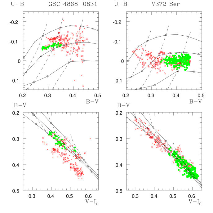
Figure 2: Colour-colour diagrams $(U-B)$-$(B-V)$ and $(B-V)$-$(V-I_{C})$. The panels on the left and right show GSC 4868-0831 and V372 Ser, respectively. The solid green circles and red crosses denote that ${\rm C}^{\rm(I)}$ is satisfied and is not satisfied, respectively. The iso-$T_{\rm e}$ and iso-$\log g_{\rm e}$ lines of the ATLAS models (Kurucz, 1997) are interpolated to $E(B-V)$ and [M] as given in Table 3. The lines with open squares, triangles, circles denote $\log g_{\rm e}=4.5,3.5,2.5\;{\rm cms}^{-2}$, respectively. The dashed lines from left to right denote $T_{\rm e}=7500,7000,6500$ K.

3 Metallicity, reddening

The physical quantities, especially $\log g_{\rm e}$, derived from photometry depend on [M] and $E(B-V)$. [M] is identical with the parameter of the ATLAS models (Kurucz, 1997). It is given on the solar scale (i.e. ${\rm[M]}=0$ dex for the solar composition). Various methods to determine [M] and $E(B-V)$ are summarized in Liu & Janes (1990), none of which is applicable for our stars except for the upper limit of $E(B-V)$, which can be found from the maps of Burstein & Heiles (1982) and from the diffuse infrared background (DIRBE, Schlegel, Finkbeiner, & Davies 1998). The precise values are of primary importance because we use $g_{\rm e}$, $T_{\rm e}$ in the Euler equation of hydrodynamics. Therefore, we have to use the photometric variation method described in Barcza & Benkő (2009) and Paper I: [M] and $E(B-V)$ are found from the best fit of the observed and theoretical colour indices of the ATLAS models (Kurucz, 1997).

When observing variable stars, we have a sum of the random scatter and temporal physical change in the colour indices, the effect of the temporal physical change manifests itself in increasing $\Delta\log g_{\rm e}$ and $\Delta T_{\rm e}$. To minimize this source of systematic error, $N^{\rm(I)}$ phases must be selected when the photometric condition ${\rm C}^{\rm(I)}$ of the QSAA is satisfied. The averages

$$\langle\Delta\log g_{\rm e}\rangle_{N^{\rm(I)}} = {1\over{N^{\rm(I)}}}\sum_{j=1}^{N^{\rm(I)}}\Delta\log g_{{\rm e},j},$$ (2)

$$\langle\Delta T_{\rm e}\rangle_{N^{\rm(I)}} = {1\over{N^{\rm(I)}}}\sum_{j=1}^{N^{\rm(I)}}\Delta T_{{\rm e},j}$$ (3)

must be minimized as a function of [M] and $E(B-V)$.

The application is straightforward for the comparison stars by setting $N^{\rm(I)}=1$ and $\log g_{\rm e}=\log g$ because their atmosphere is static and the observed colour indices have a random scatter only. For orientation, $E(B-V)$, [M], $T_{\rm e}$, $\log g$, $\vartheta$ of comparison stars of approximately the same colours were determined using our method. The minimal value of the scatters $\Delta\log g$, $\Delta T_{\rm e}$ shows the effect of the random error of the colour indices. The averages for the different comparison stars suggest that the limits of the applicability of the QSAA are $\Delta T_{\rm e}\la 5$ and $\Delta\log g\la 0.04$ in our observational material. That is, $\mbox{C}^{\rm(I)}$ is satisfied in the phases where $\Delta T_{\rm e}$ and $\Delta\log g_{\rm e}$ do not exceed these limits.

The numerical results are $\langle\Delta\log g_{\rm e}\rangle_{39}=0.022\pm 0.001$ $\langle\Delta T_{\rm e}\rangle_{39}=8.6\pm 0.5$ K for GSC4868-0831, $\langle\Delta\log g_{\rm e}\rangle_{249}=0.031\pm 0.002$, $\langle\Delta T_{\rm e}\rangle_{249}=6.2\pm 0.2$ K for V372 Ser. The $\Delta T_{\rm e}\la 5$ K limit from the comparison stars is exceeded slightly. The excess originates from the inclusion of phases into $N^{\rm(I)}$, which satisfy $\Delta\log g_{\rm e}\la 0.04$ but violate $\Delta T_{\rm e}\la 5$ K because of the temporal neighbourhood of an atmospheric shock. The results are summarized in Table 3. The atmospheres of both variables are moderately metal deficient.

3.1 The observed $U-B$, $B-V$, $V-I_{C}$ colour indices

The observed $(U-B)$-$(B-V)$, $(B-V)$-$(V-I_{C})$ colour-colour diagrams are plotted in Fig. 2. The phases are plotted separately when ${\rm C}^{\rm(I)}$ is or is not satisfied (green circles and red crosses, respectively). The theoretical colour-colour relations of the ATLAS models (Kurucz, 1997) belonging to some characteristic $\log g_{\rm e}$ and $T_{\rm e}$ were interpolated for the [M] and $E(B-V)$ values of the variables. These are the lines in Fig. 2. Before discussing the hydrodynamic details, we can draw some conclusions from the data plotted in Fig. 2.

• The segregation of the colour indices satisfying ${\rm C}^{\rm(I)}$ is clearly seen. However, a remarkable dichotomy is obvious: the phases of GSC 4868-0831 satisfying ${\rm C}^{\rm(I)}$ are concentrated in the blue $B-V$ domain, while those of V372 Ser populate the red $B-V$ region.

• Within the observational scatter, the $(B-V)$-$(V-I_{C})$ values of V372 Ser are in the domain of $2.5<\log g_{\rm e}<4.5$. A considerable number of $(B-V)$-$(V-I_{C})$ pairs of GSC 4868-0831, which do not satisfy ${\rm C}^{\rm(I)}$, are significantly below this domain indicating $\log g_{\rm e}\gg 4.5$. A combination of [M] and $E(B-V)$ could not be found that would have shifted every pair into a common domain of $\log g_{\rm e},T_{\rm e}$, [i.e. ${\rm C}^{\rm(I)}$ is more strongly violated by the atmosphere of GSC 4868-0831].

• As indicated by the difference in $\overline{\log g_{\rm e}}=3.69,3.24$ (Table 3), the surface gravity of GSC 4868-0831 must be by a factor $\approx 3$ larger than that of V372 Ser, [i.e. GSC 4868-0831 is a subgiant rather than a giant star].

4 Distance, mass and atmospheric kinematics

The dynamical equation of the pulsation of an atmosphere with spherical symmetry was derived in Paper I from the Euler equation of hydrodynamics. Its most convenient form is

$${{\cal M}_{\rm a}\over{d^{2}}}={{\vartheta^{2}(t)}\over{G}}\Bigl{[}g_{\rm e}(t)-a(r,t)-a^{\rm(dyn)}(r,t)\Bigr{]},$$ (4)

where $a(r,t)=\partial v/\partial t+v(\partial v/\partial r)$, $G$ is the Newtonian gravitation constant. The dynamical correction $a^{\rm(dyn)}(r,t)$ accounts for the difference between the accelerations of a static and a dynamical model atmosphere at time $t$. The solution of the continuity equation for mass conservation in the frames of QSAA resulted in a series expansion

$$v(r,t)={\dot{\vartheta}}d-{1\over{h_{0}}}{{\partial h_{0}}\over{\partial t}}r+\cdots,\>\>r\la R.$$ (5)

This was given in Paper I with detailed explanations for the symbols in Eqs. (4), (5). $R$ is the stellar radius [i.e. the radius of approximately zero optical depth], $\vartheta=R/d$, the dot denotes a differentiation with respect to $t$, $h_{0}=\mu g_{\rm e}(t)/{\cal R}T(R,t)$ is the reciprocal barometric scaleheight at $r\approx R$.

The velocity profile (5) was introduced in Eq. (4) for each epoch $j$, $j=1,...,N$ and ${\cal M}_{\rm a}$ and $d$ were determined in four steps. In comparison with the technique in Paper I, the refinement of the solution of Eq. (4) was rendered possible by the large number of the observed points. ($N=280$ and $529$ for GSC 4868-0831 and V372 Ser, respectively.)

• The photometric inverse problem [i.e. the conversion of the $UBV(RI)_{C}$ observations to $\vartheta,\log g_{\rm e}$ and $h_{0}$] was solved for $N$ observations, as described in Paper I, and the $N^{\rm(I)}$ phases were found that satisfied ${\rm C}^{\rm(I)}$. Polynomial fits of degree 7-10 were calculated for $\vartheta(t),\log g_{\rm e}(t),h_{0}(R,t)$. One polynomial was sufficient for the whole time interval (of length $<0\aas@@fstack{d}3$) if the atmosphere was in a shock-free state; $\leq 3$ polynomials were necessary in a strongly shocked phase.

• Epochs of number $n$ could be selected by differentiation of $\vartheta(t)$ when $v(r,t)/d={\dot{\vartheta}}+\cdots\approx\mbox{constant}$, and the angular acceleration $a^{\rm(ang)}(r,t)=a(r,t)/d={\ddot{\vartheta}}-{\dot{\vartheta}}h_{0}^{-1}(\partial h_{0}/\partial t)+\cdots\approx 0$ over the whole atmosphere because the leading terms in $v/d$ and $a/d$ are large in comparison to the rest. We can well assume that ${\rm C}^{\rm(II)}$ was satisfied in these shock-free intervals if the atmosphere was in free fall [i.e. $a^{\rm(dyn)}(r,t)\approx 0$ holds in their vicinity]. This is the descending branch in the light curve. Eq. (4) reduces, in these epochs, to

  $$({\cal M}_{\rm a}d^{-2})_{i}=G^{-1}g_{\rm e}(t_{i})\vartheta^{2}(t_{i}),\>i=1,...,n,$$ (6)

  $n$ is given in Table 4. These $n$ epochs form a subset of the $N^{\rm(II)}$ epochs satisfying $\mbox{C}^{\rm(II)}$.

  We remark that $a^{\rm(dyn)}(r,t)\approx 0$ might not be expected in the minimum and ascending branch of the light curve because there are atmospheric layers moving in opposite direction [i.e. the atmosphere is not in free fall]. The approximation (6) is not valid in these phases in spite of $a^{\rm(ang)}\approx 0$ for a short time when the rapidly changing $a^{\rm(ang)}(r,t)$ has a sign change. These shocked phases were therefore not included in $i=1,2,...,n$.

  The right hand side of Eq. (6) consists of quantities derived directly from the photometry without differentiations of the polynomial fits. This can be determined with an accuracy of $\leq 0.15$ from the $UBV(RI)_{C}$ photometry in each $t_{i}$.

• By introducing the averaged value

  $${{\cal M}_{\rm a}\over{d^{2}}}={1\over n}\sum_{i=1}^{n}\Bigl{(}{{\cal M}_{\rm a}\over{d^{2}}}\Bigr{)}_{i}$$ (7)

  we reduce Eq. (4) to an algebraic equation for unknown $d_{j}$ at any $t_{j},\>j=1,...,N$ if $a^{\rm(dyn)}=0$; the largest term is linear in $d_{j}$. These $N$ equations can be solved by elementary operations for all $j$. The distance was obtained from

  $$d(N)={1\over N}\sum_{j=1}^{N}d_{j}.$$ (8)

  At this step, an averaged dynamical correction

  $$\overline{a^{\rm(dyn)}}(R,N) = {1\over N}\sum_{j=1}^{N}a^{\rm(dyn)}(R,t_{j})$$ (9)

  $$= {1\over N}\sum_{j=1}^{N}\Bigl{[}g_{\rm e}(t_{j})-{{G{\cal M}_{\rm a}}\over{\vartheta^{2}(t_{j})d^{2}}}-a(R,t_{j})\Bigr{]}$$

  was defined with ${\cal M}_{\rm a}d^{-2}$ and $d(N)$ from Eqs. (7) and (8) facilitating the reduction of the number of the equations (4) to be solved.

• To obtain the final $d(N^{\rm(II)})$ the step (iii) was repeated, reducing $N$. One or two iterative steps were necessary to obtain $\overline{a^{\rm(dyn)}}(R,N^{\rm(II)})\ll\overline{g_{\rm s}[R(t)]},$ and $|a^{\rm(dyn)}(R,t_{j})|_{j=1,...}\la 0.3\overline{g_{\rm s}[R(t)]}$ where $g_{\rm s}[R(t)]=G{\cal M}_{\rm a}R^{-2}(t)$. That is, the roots $d_{j}$ of Eq. (4), originating from the $t_{j}$ intervals, were removed from Eq. (8) which produced outlier values with $a^{\rm(dyn)}(R,t_{j})\ga 0.3g_{\rm s}[R(t_{j})]$. The results of the iterative steps are given in Table 4.

Table 4: The results from steps (i)-(iv).

$\{E(B-V),[M]\}$	$n$	${\cal M}_{\rm a}d^{-2}\times 10^{7}$	$d$	${\cal M}_{\rm a}$	$\overline{a^{\rm(dyn)}}(R,t)$	$N$
${\rm[mag],[dex]}$		[${\cal M}_{\odot}\mbox{pc}^{-2}$]	[pc]	[${\cal M}_{\odot}$]	[$\mbox{ms}^{-2}$]
GSC 4868-0831
$\{0.008,-1.05\}$	7	$40.3\pm 6.7$	$451\pm 99$	$.82\pm.36$	$-58.4$	280
			$467\pm 16$	$.88\pm.06$	$0.10$	$21^{\ast}$
V372 Ser
$\{0.003,-0.53\}$	20	$6.12\pm.31$	$1183\pm 74$	$0.85\pm.13$	$13.90$	529
			$1020\pm 87$	$0.63\pm.12$	$1.64$	249
			$964\pm 81$	$0.57\pm.10$	$0.41$	$135^{\ast}$

Note. The ^∗ indicates $N^{\rm(II)}$; $|a^{\rm(dyn)}|<3\mbox{ms}^{-2}$ is satisfied for all $t_{j},j=1,...,N^{\rm(II)}$.

The interval of the search for roots of Eq. (4) was limited to

$$d_{j}\leq d_{\rm max}=g_{\rm e}{\ddot{\vartheta}}^{-1}_{\rm max}.$$ (10)

To obtain this upper limit, we took into account only the linear term of the acceleration when the atmosphere is hit by the strongest shock wave; this is the state of maximal compression. At this epoch the atmosphere is just reversed from inward to outward motion. That is, $v(\partial v/\partial r)\approx 0$, $\partial v/\partial t={\ddot{\vartheta}}d>0$, $R$ is minimal, the deceleration by the static gravity is negligible ($g_{\rm s}\ll\partial v/\partial t$) and, furthermore, $a^{\rm(dyn)}\approx 0$ was supposed. However, the upper limit $d_{\rm max}$ was taken into account only if the satisfaction of these conditions plus, ${\rm C}^{\rm(I)}$ and ${\rm C}^{\rm(II)}$, was verified afterwards.

4.1 Numerical results

Our observations provided 10 light curve segments of sufficient length and quality to calculate the polynomial fits of $\log g_{\rm e}(t),T_{\rm e}(t)$ and $\vartheta(t)$ for both stars. The order of magnitude limits were found to be $-10^{-20}<{\rm O}[a^{\rm(ang)}]<10^{-18}\mbox{rad}\cdot\mbox{s}^{-2}$ for both stars. The acceleration-free intervals can be found for Eq. (7) from quantities that are of the form $f(\vartheta)+{\rm O}(d^{-1})$.

The results from step (i), [M] and $E(B-V)$ are given in Table 3. The results from steps (ii)-(iv) and the final $d$ and ${\cal M}_{\rm a}$ are summarized in Table 4. The asterisk in the last column denotes the value of $N^{\rm(II)}$.

The position of the stars in a theoretical HRD was calculated by

$$T_{\rm eq} = \langle\vartheta^{2}T_{\rm e}^{4}\rangle^{1/4}\langle\vartheta\rangle^{-1/2},$$ (11)

$$L_{\rm eq} = 4\pi\sigma d^{2}\langle\vartheta^{2}(\varphi)T_{\rm e}^{4}(\varphi)\rangle$$ (12)

(Carney, Strom & Jones, 1992). The numerical values are given in Table 5. The remarkably small error of $T_{\rm eq}$ originates from the sum of the scatter of $T_{\rm e}$, determined from the different colour-colour combinations and the scatter of $\vartheta$ when it is determined from the brightness in $V,R_{C}$ and $V$ plus bolometric correction and the Stefan-Boltzmann law. The components of the error of $L_{\rm eq}$ are composed of errors from $\langle\vartheta^{2}T_{\rm e}^{4}\rangle$, ${\cal M}_{\rm a}d^{-2}$ and $d$, respectively. The numerical values are $\pm 0.18,\pm 0.35,\pm 0.70$ for GSC 4868-0831 $\pm 0.2,\pm 1.3,\pm 3.7$ for V372 Ser. A summary of the parameters is given in Table 5.

The error of the magnitude averaged $\langle M_{V}\rangle$ was estimated from sum of the errors of ${\cal M}_{\rm a}d^{-2}$ and $d$ in Table 4.

Fig. 3 presents an insight into the variable quantities of the atmosphere at a shock-free and a shocked phase for both stars. The segment of $V(t)$ is plotted in the uppermost row for orientation. The scatter of $T_{\rm e}(t)$ (row 2) reflects the scatter in our photometry. $R(t)$ and the velocities and accelerations were computed from the smoothed $\vartheta(t)$ and $\log g_{\rm e}(t)$ using $d$ and ${\cal M}_{\rm a}$ from Table 4.

We see a considerable gradient of $v(r)$ for GSC 4868-0831 at HJD$\ga 2454829.6$, just when a descending branch of the light curve ended. The deeper layers were moving outwards much faster because the atmosphere was hit by a shock wave, and the velocity excess reached $\approx 25$ kms ^-1. Otherwise $|v(R)-v(R-h_{0}^{-1})|\approx$ a few km s ^-1 was found for both stars.

Row 5 is a plot of $g_{\rm s}(R,t)$. The different types of GSC 4868-0831 and V372 Ser are obvious if we compare $R(t)$ and $g_{\rm s}(R,t)$; GSC 4868-0831 is a subgiant star while V372 Ser has a true RRd character. The components of the acceleration are plotted in row 6 in the relative units $q_{d}=a^{(\rm dyn)}(R,t)g^{-1}_{s}(R,t)$, $q_{r}={\ddot{R}}(R,t)g^{-1}_{s}(R,t)$, $q_{a}=a(R,t)g^{-1}_{s}(R,t)$. Here, $|q_{d}|\la 0.3$ is the domain when ${\rm C}^{\rm(II)}$ is satisfied if the light curve is not in ascending branch. The rapid changes of the components were not smoothed out, especially those of $q_{d}$ of V372 Ser at HJD$>2454250.57$. These originate partly from violating ${\rm C}^{\rm(I)}$, and partly from the stronger effect of the thermic shock on the more dilute atmosphere of V372 Ser. $q_{d}\ga 10$ means that $g_{\rm e}$ derived from the photometry has a very loose connection with the atmospheric kinematics. This must be corrected by a term $\gg g_{\rm s}$ to obtain the actual acceleration in the atmosphere.

Figure 3: The variable physical parameters of GSC 4868-0831 and V372 Ser in descending and ascending branches of the $V$ light curve. Row 1: light curves $V(t)$. Row 2: $T_{\rm e}(t)$. Row 3: $R(t)$. Row 4: solid lines: $v(R,t)$, dotted lines: $v(R-h_{0}^{-1},t)$. Row 5: $g_{\rm s}(R,t)$. Row 6: relative accelerations (solid lines: $q_{d}=a^{(\rm dyn)}(R,t)g^{-1}_{s}(R,t)$, dotted lines: $q_{r}={\ddot{R}}(R,t)g^{-1}_{s}(R,t)$, dashed lines: $q_{a}=a(R,t)g^{-1}_{s}(R,t)$).

5 Discussion

5.1 Remarks on the photometric inverse problem

Because of the lack of high-dispersion spectra the relations

$${\cal P}=f({\rm CI}_{1},{\rm CI_{2}}...)$$ (13)

play a crucial role. Here, ${\cal P}$ and $\mbox{CI}_{i}$ denote an astrophysical quantity and colour index, respectively. For example, a particular form of $f$ belongs to ${\cal P}=T_{\rm e}$, ${\cal P}=\log g$, etc. These are given in tabular form for the ATLAS models (Kurucz, 1997), and their parameters are $E(B-V)$, [M], etc. (As emphasized in Sec. 3, [M] is on the solar scale and $f$ would have another form for a peculiar atmospheric chemical composition.)

The derived fundamental parameters depend on the reddening and metallicity. A larger $E(B-V)$ leads to larger $\log g$ and $T_{\rm e}$, the dependence on [M] is similar, but to a lesser extent. The essence of our method is that we search for the minimal standard errors $\Delta\log g_{\rm e},\Delta T_{\rm e}$ of $\log g_{\rm e},T_{\rm e}$ from some 30 colour index pairs as a function of [M] and $E(B-V)$. This method is self-consistent to the highest degree from an astrophysical point of view. We use all colour information of the atmospheric models to determine the relevant parameters and quantities. In doing so, we can avoid the systematic errors inherent to an arbitrary choice of relations such as, for example, $T_{\rm e}$-$(V-I_{C})$, ${\rm[M/H]}$-$(B-V)$, (e.g. Dékány et al. 2008). In addition, we do not use semi-empirical calibrations at all (e.g. the $T_{\rm e}$-colour index relations derived for non-variable main sequence stars of normal chemical composition and, as next step, generalized to variable giant stars with large metal deficiency, Clementini et al 2000).

Of course, in comparison with a line by line analysis of high-dispersion spectroscopy, a multicolour photometry is sensitive only to the general shape of the optical flux of the star. However, it is possible to find the model atmosphere by reproducing the continuum flux in the visible wavelength interval. Our method can provide a global parameter of the chemical composition in the atmosphere summarized as metallicity [M]. This [M] is the most suitable for our purposes, because it accounts for the effect of all elements on the optical continuum, including those that do not have lines. Of course, it might differ from the overall metallicity of the star (used in the theory of stellar structure, as the pulsation does not stir up the deepest layers where the nuclear reactions take place) or from the averaged metallicity derived from high dispersion spectroscopy.

The fields are at high Galactic latitude: GSC 4868-0831, $b=+24\degr$; V372 Ser, $b=+45\degr$. Their reddening is very small, and therefore the parameters ($\log g_{\rm e}$, $T_{\rm e}$, $d$, ${\cal M}_{\rm a}$) reported in Section 4 are lower limits at the same time if [M] is fixed. The upper limits are $E(B-V)<0.023,0.085$ (Schlegel, Finkbeiner, & Davies, 1998), or $E(B-V)<0.03,0.045$ Burstein & Heiles 1982, respectively. We attribute our smaller $E(B-V)$ to two factors: our method measures the reddening of a point source and the excess reddening must originate from a region beyond GSC 4868-0831, V372 Ser, and the comparison stars.

The reddening $E(B-V)=0.085$ of V372 Ser derived from the DIRBE differs from our value above the $5\sigma$ level. Taking this large $E(B-V)$ would result in an unacceptable increment from $\langle\Delta T_{\rm e}\rangle_{249}=6.2\pm 0.2$ to $8.2\pm 0.4$. The parameters would increase to $\overline{\log g_{\rm e}}=4.11$, $\overline{T_{\rm e}}=7092$ leading to a mass above $5{\cal M}_{\odot}$ which cannot be reconciled with any actual theoretical knowledge about pulsating stars. Therefore, $E(B-V)>0.006$ can be ruled out.

5.2 The use of $U$ observations

Concerning GSC4868-0831, an interesting result can be seen from Fig. 2: the phases satisfying and not satisfying ${\rm C}^{\rm(I)}$ segregate clearly in the colour-colour diagrams and completely different $T_{\rm e}(t)$ and $\log g_{\rm e}(t)$ are obtained for these phases if a $BVI_{C}$ photometry only is used as input. Fig. 2 demonstrates that reliable $T_{\rm e}(t)$ and $g_{\rm e}(t)$ can be determined only if colour indices containing $U$ are used in the $T_{\rm e}$, $\log g_{\rm e}$ domain of RR stars. The use of one colour index or $BVI_{C}$ photometry only is not sufficient and can be misleading, even if it is limited to determining $T_{\rm e}$ only.

Furthermore, our $U$ observations might reveal the subgiant character of GSC 4868-0831 which was not suspected previously (Wils & Otero 2005, Wils, Lloyd & Bernhard 2006, Szczygieł & Fabryczky 2007). An important conclusion has emerged that it is not possible to determine the luminosity class of a pulsating star if only periods or period ratio are available. Multicolour observations, covering the ultraviolet, are needed to classify DM pulsators properly.

5.3 Remarks on the QSAA

We have to emphasize that $L_{\rm eq}$ and $T_{\rm eq}$ are first approximations from Eqs. (11) and (12) because some elements of the averaging were obtained assuming QSAA in phases when ${\rm C}^{\rm(I)}$ was violated. Qualitative considerations suggest a positive correction to $T_{\rm e}(t)$ of QSAA in the shocked phases when excess radiation and dissipation exist from shock waves. Corrections emerging from a dynamical model atmosphere would not modify the main fundamental parameters ${\cal M}_{\rm a}$ and $d$ because they were determined from phases when both quantitative conditions of the validity of QSAA were satisfied. ${\cal M}_{\rm a}$ and $d$ can be considered as well substantiated empirical data from the ATLAS static model atmospheres plus some basic hydrodynamics. Dynamical model atmospheres are beyond the scope of this series of papers.

The sampling of the quasi-repetitive curves introduced negligible error, which can be estimated by comparing $T_{\rm e}$ and $\vartheta$ from the fitted colour curves (Benkő & Barcza, 2009) with those from the $N=529$ observations of V372 Ser.

We remark that $d=(1145\pm 73)$ pc, ${\cal M}_{\rm a}=(0.83\pm.17){\cal M}_{\odot}$ are the results for $\{E(B-V)=0.003,[M]=-0.53\}$ if the UAA is applied, that is, if $\partial v/\partial r=0$ is assumed in Eq. (4) (and, as a consequence, $\vartheta=R/d$ and $\partial v/\partial t={\ddot{\vartheta}}d$). This distance and the change of ${\cal M}_{\rm a}d^{-2}=6.12\pm.31\rightarrow 7.64\pm.82$ gives $L_{\rm eq}^{(\rm UAA)}=42.8L_{\odot}$ which put V372 Ser in a position just at the lower limit of stable DM pulsation (Szabó, Kolláth & Buchler, 2004). Of course, the physical input of the UAA is much less than that of our extended hydrodynamic treatment represented by Eqs. (4), (5). In spite of the better agreement, the data from UAA must not be accepted because the UAA is a rigid and less realistic approximation in comparison with a compressible model atmosphere.

Figure 4: The positions of the stars in a theoretical HRD. The square denotes SU Dra, (with $[L_{\rm eq},T_{\rm eq}]$ were taken from Paper I), The triangle and circle denote V372 Ser and GSC 4868-0831, respectively. The solid lines from left to right denote the blue and red edges of the instability strip. The dashed line denotes the zero age horizontal branch of M3 (Silva Aguierre et al., 2008).

5.4 Classification of the stars

The positions of our stars and SU Dra in a theoretical HRD, (i.e. $[L_{\rm eq},T_{\rm eq}]$) are plotted in Fig. 4. For orientation, the instability strip and the zero age horizontal branch of the metal deficient ([M]$\approx-1.6$) globular cluster M3 (NGC 5272) are shown (Silva Aguierre et al., 2008). We emphasize that $[L_{\rm eq},T_{\rm eq}]$ correspond to $L$ and $T_{\rm e}$ of non-variable stars, and they can be directly compared with those from the theoretical studies on stellar structure, pulsation and evolution. The only source of error is the difference of $T_{\rm e}(t)$ and $\vartheta(t)$ in Eqs. (11, 12) from QSAA and dynamical model atmospheres, respectively. An error has not been propagated into the position of the star by semi-empirical relations like $\overline{T_{\rm e}}$-$\overline{(B-V)}$ etc.

The period ratios $P_{1}/P_{0}$ are $=0.7443$ and $0.7450$ for V372 Ser and GSC 4868-0831, respectively. These are in the canonical range of RRd stars, as ${\cal M}_{\rm a}$ of V372 Ser is also. The equilibrium effective temperatures of both stars are in the $5630<T_{\rm eq}<7080$ K interval where DM pulsation can be stable. The results of our analysis confirm that V372 Ser is a true RRd star. However, it is subluminous by a factor of $\approx 2\mbox{-}3$ in comparison with the pulsation models of RRd stars (Szabó, Kolláth & Buchler, 2004).

${\cal M}_{\rm a}$ of GSC 4868-0831 exceeds somewhat the canonical mass of RRd stars; its subluminosity is even larger, $\approx 4\mbox{-}5$ and its radius is less than half that of an RR star. The periods exclude its identification as DM SX Phe star. To the best of our knowledge, GSC 4868-0831 is the first known subgiant star pulsating in two modes of large amplitude. It is slightly ($\approx 1$ mag) above the zero age main sequence of normal chemical composition, and it is below the extension of the instability strip of M3.

6 Conclusions

We have reported 302 $UBV(RI)_{C}$ observations of GSC 4868-0831. To the best of our knowledge, this is the second DM pulsating star with well documented photometric behaviour in the optical and near ultraviolet bands.

We have determined, for the first time, fundamental parameters of DM pulsators using only the theory of stellar atmospheres. Our method is purely photometric; the eventual uncertainty of observing radial velocities and their conversion into the reference frame in the centre of the star can be avoided using our method. Our method has made extensive use the ATLAS model atmospheres and some basic hydrodynamics. Our astrophysical input is completely different from the theory of stellar pulsation and evolution. Therefore, our method can be used as a check or challenge for these more involved theories.

We have summarized our results in Table 5. We have found the surprising result that GSC 4868-0831 is not an RRd star, but a subgiant star pulsating in two modes. We have found a significant subluminosity of the RRd star V372 Ser in comparison with the luminosity from present day theory of stellar pulsation. These objects must be considered as a challenge to extend the search for stable DM pulsation. Qualitative considerations suggest that dynamical model atmospheres would have higher $T_{\rm eq}$ and $L_{\rm eq}$; both corrections would shift the points in Fig. 4 upwards and to the left with respect to their position from QSAA. However, we must not forget that our results from static ATLAS model atmospheres have yielded the ratio ${\cal M}_{\rm a}d^{-2}$ and $d$ from phases when a dynamical model atmosphere is not necessary (i.e. QSAA is a reliable approximation of the pulsating atmosphere). We are faced with the dilemma that there is either subluminosity with acceptable mass or acceptable luminosity with too large mass if we are to reconcile these parameters from the present-day theory of stellar pulsation.

Table 5: Summary of the parameters.

	GSC 4868-0831	V372 Ser
$P_{0}$	$0\aas@@fstack{d}5649^{\ddagger}$	$0\aas@@fstack{d}4712289^{\dagger}$
$A_{0}$	$0.07271^{\ddagger}$ mag	$0.1534^{\dagger}$ mag
$P_{1}$	$0\aas@@fstack{d}42085^{\ddagger}$	$0\aas@@fstack{d}3507310^{\dagger}$
$A_{1}$	$0.15815^{\ddagger}$ mag	$0.2059^{\dagger}$ mag
$E(B-V)$	$0.008\pm.002$ mag	$0.003\pm.003$ mag
${\rm[M]}$	$-1.05\pm.10$ dex	$-0.53\pm.05$ dex
$d$	$467\pm 16$ pc	$964\pm 81$ pc
$\langle M_{V}\rangle$	$+2.40\pm.24$ mag	$+1.58\pm.22$ mag
${\cal M}_{\rm a}$	$0.88\pm.06{\cal M}_{\odot}$	$0.57\pm.10{\cal M}_{\odot}$
$R_{\rm min}$	$1.97R_{\odot}$	$4.07R_{\odot}$
$R_{\rm max}$	$2.05R_{\odot}$	$4.40R_{\odot}$
$T_{\rm eq}$	$6924\pm 35\mbox{K}$	$6722\pm 20\mbox{K}$
$L_{\rm eq}$	$8.97\pm 1.23L_{\odot}$	$21.9\pm 5.2L_{\odot}$

Notes.

^†: From Benkő & Barcza (2009).

^‡: determined from the $V$ observations.

Appendix A Description of the program package BBK

The package BBK is designed to extract the fundamental parameters of RR stars from high-quality $UBV(RI)_{C}$ observations. A brief description and some technical details are given here.

It is important to have the colours and colour indices as close as possible to the international colour system which was applied by Kurucz (1997) in order to convert the physical fluxes of the ATLAS models to the stellar magnitude and colour system. An error (or errors) in the colour indices can lead to false results. To obtain reliable results, some $N\ga 300$ five colour observations are needed. These must be distributed uniformly over a representative light curve because the physical quantities $\vartheta$, $h_{0}$ must be differentiated.

Proper use of the program package requires basic knowledge of absolute stellar photometry, the theory of stellar atmospheres and hydrodynamics. As Kurucz (1997) said: ’Neither the programs nor data are black boxes. You should not be using them if you do not have some understanding of the physics and of the programming in the source code.’ This warning is appropriate for BBK.

BBK consists of FORTRAN programs, z-shell scripts, input files, data files, and a manual (Barcza, 2011). UNIX or LINUX environment, installation of a FORTRAN compiler, z-shell, graphical packages (e.g. SUPERMONGO, or GNUPLOT) are necessary. Five steps are involved, a detailed description of which can be found in the manual. Inspection, evaluation, plots of the partial results are necessary before continuing to the next step.

Step (I) The atmospheric metallicity and the interstellar reddening of the star are determined from selected phases when the atmosphere is free of shocks (i.e. from colour indices in the descending branch).

Step (II) The conversions

$$f({\rm CI}_{1},{\rm CI_{2}}...)\rightarrow{\cal P}$$ (14)

are executed to select the static ATLAS models with the best fit to the observed and theoretical colour indices to obtain $\log g_{\rm e}$ and $T_{\rm e}$ as a function of phase. The variation of $\vartheta$ is determined by comparing the physical fluxes of the star with those of the selected theoretical models. The physical fluxes $V$, $R_{C}$, $V+$ bolometric correction are used, those of the star are calculated from the absolute calibration of Vega (Tüg, White & Lockwood, 1977).)

Step(III) Polynomial fits are calculated to obtain $\log g_{\rm e}$, $T_{\rm e}$, $h_{0}$, angular velocity and acceleration ${\dot{\vartheta}},{\ddot{\vartheta}}$ as a function of phase. The upper limit $d_{j}\leq d_{\rm max}=g_{\rm e}{\ddot{\vartheta}}^{-1}_{\rm max}$ must be fixed by inspecting ${\ddot{\vartheta}}$ as a function of phase.

Step(IV) The fits are introduced in the Euler equation of hydrodynamics to determine the angular acceleration and to find the acceleration-free phases of the atmosphere. The transient acceleration-free intervals in the ascending branch (i.e. in the shocked phases) must be manually deleted from the averaging to find ${\cal M}_{\rm a}d^{-2}$.

Step(V) $\vartheta$, ${\dot{\vartheta}}$, ${\ddot{\vartheta}}$, $h_{0}$, $\partial h_{0}/\partial t$, $g_{\rm e}$ and ${\cal M}_{\rm a}d^{-2}$ are introduced in Eqs. (4,5) and Eq. (4) is solved for $d$ with the whole (or partial) set containing $N$ (or $<N$) phase points. The upper limit $a^{\rm(dyn,\;upper\;limit)}$ must be specified to exclude the phase points from the final solution for $d$ [i.e. from $N^{\rm(II)}$] to achieve $|a^{\rm(dyn)}|<a^{(\rm dyn,\;upper\;limit)}$ in all phase points giving $d$. One or two runs might be necessary with decreasing $N$.

References

- Barcza (2002) Barcza S., 2002, A&A 384, 460
- Barcza (2003) Barcza S., 2003, A&A 403, 683
- Barcza (2006) Barcza S., 2006, Comm. Konkoly Obs. No. 104, p. 149
- Benkő & Barcza (2009) Benkő J. M., Barcza S., 2009, A&A, 497, 481
- Barcza & Benkő (2009) Barcza S., Benkő J. M., 2009 in ”Stellar Pulsation: Challenges for Theory and Observation” Eds. J. A. Guzik and P. Bradley AIP Conf. Proc. 1170, pp 250-252
- Barcza (2010) Barcza S., 2010, MNRAS, 406, 486, Paper I
- Barcza (2011) Barcza, S., 2011, Konkoly Obs. Occasional Technical Notes No. 14
- Burstein & Heiles (1982) Burstein D., Heiles C., 1982, AJ, 87, 1165