Crosslinked biopolymer bundles: crosslink reversibility leads to cooperative binding/unbinding phenomena

Abstract

We consider a biopolymer bundle consisting of filaments that are crosslinked together. The crosslinks are reversible: they can dynamically bind and unbind adjacent filament pairs as controlled by a binding enthalpy. The bundle is subjected to a bending deformation and the corresponding distribution of crosslinks is measured. For a bundle consisting of two filaments, upon increasing the bending amplitude, a first-order transition is observed. The transition is from a state where the filaments are tightly coupled by many bound crosslinks, to a state of nearly independent filaments with only a few bound crosslinks. For a bundle consisting of more than two filaments, a series of first-order transitions is observed. The transitions are connected with the formation of an interface between regions of low and high crosslink densities. Combining umbrella sampling Monte Carlo simulations with analytical calculations, we present a detailed picture of how the competition between crosslink shearing and filament stretching drives the transitions. We also find that, when the crosslinks become soft, collective behavior is not observed: the crosslinks then unbind one after the other leading to a smooth decrease of the average crosslink density.

I Introduction

The cytoskeleton is a complex meshwork made of long elastic filaments coupled together with the help of numerous, rather compact crosslinking proteins alb94 . An important aspect of cytoskeletal assemblies is their dynamic nature, which allows them to react to external stimuli and adapt their internal structure and mechanical properties according to the needs of the cell. The reversible nature of crosslink binding is an important mechanism that underlies these dynamical processes. For example, living cells show complex rheological properties that range from fluidization to reinforcement under stresstrepat2007Nature ; Fernandez2006BPJFibroblast , and reversible bonds between cytoskeletal filaments have been proposed as key mechanisms in mediating between these contradicting behaviors KollmannsbergerReview2011 ; wolffNJP2010 . Similar effects are believed to be important for the rheological properties of reconstituted F-actin networksbausch06 ; LielegSoftMatter2010 ; KaszaCOCB2007 , in particular at low frequencies that correspond to the lifetime of the crosslink-mediated bondlielegPRL2008Transient ; broederszPRL2010Linker .

Another important class of cytoskeletal assemblies are filament bundles. Crosslinked F-actin bundles form primary structural components of a broad range of cytoskeletal structures including stereocilia, filopodia, microvilli or the sperm acrosome. Type and properties of the crosslinking protein allow the cell to tailor the dimensions and mechanical properties of the bundles to suit specific biological functions. In particular, the mechanical properties of these bundles play key roles in cellular functions ranging from locomotionmogilnerBPJ2005 ; atilganBPJ2006 ; vignejvic2006JCellBiol to mechanotransductionhudspeth1977PNAS , and fertilizationschmid2004Nature .

In-vitro experiments and modeling have emphasized the role of the crosslink stiffness in mediating bundle mechanical propertiesclaessens06NatMat ; Bathe20082955 ; PhysRevLett.103.238102 . It is less clear, however, in how far the reversibility of the crosslinking bond may affect bundle mechanical or dynamical properties. On the one hand, one expects reversible bonds to influence the conformational properties of the filaments. Examples for this dependency are the formation of kinks in the bundle contourcohenPNAS2003 ; DogicPRL2006Kinks , or an unbundling transition as the binding affinity of the crosslinks is reducedbenetatosPRE2003 ; kierfeld05PRL . Conversely, bundle conformational changes or the application of destabilizing forceskierfeldPRL2006Unzipping directly influence the binding state of the crosslinks.

The aim of this article is to deepen our understanding of this complex interplay between reversible crosslink binding and bundle mechanical and dynamical properties. We consider the nonlinear response of a reversibly crosslinked filament bundle to an imposed external force or deformation. In particular, we want to determine how the external driving is reflected in the internal degrees of freedom of the bundle, notably the binding state of the crosslinks. Combining simulations and theory we will show that, depending on the mechanical stiffness of the crosslinking agent, the fraction of bound crosslinks can display a sudden and discontinuous drop. This indicates a cooperative unbinding process that involves the crossing of a free energy barrier. Choosing the proper crosslinking protein, therefore, not only allows one to change the composite elastic properties of the bundle, but also the relevant time-scales: the latter can be tuned from the single crosslink binding rate to the (much longer) escape time over the free energy barrier (a short communication of these results was recently presented by one of us in Ref. PhysRevE.83.050902, ). We emphasize that related effects may be important in a variety of different biological contexts also. For example, cellular adhesion and locomotion are dependent on the formation of transient cell-to-matrix bondsjulianoCellAdhesionReview2002 ; Critchley2000FocalAdhesion . Simple theoretical models highlight the complex interplay between specific adhesion, mediated by the binding agent, unspecific interaction with the substrate, and cell-membrane elasticityBruinsmaSackmannPRE2000 ; weiklSoftMatterReview2009 ; SmithSeifertSoftMatter2007 ; weil.faragoEPJE2010 .

The outline of the paper is as follows. In Section II, we define and motivate our bundle model. Next, in Section III, we present our numerical results obtained in Monte Carlo simulations. In Section IV, the development of a theoretical model is described. The combined efforts of simulation and theory allow us to obtain a detailed understanding of the underlying physical mechanisms that affect the crosslink binding state. We end in Section V with a discussion of the implications and the experimental relevance of our results.

II Model

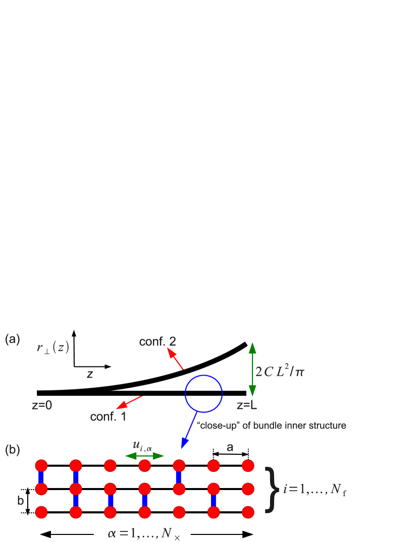
Figure 1: (a) An end-grafted bundle of length $L$ is brought from an initial unbend state (configuration 1) to a bend state (configuration 2). The bundle contour $r_{\perp}(z)$ is given by Eq. (1), where $C$ sets the bending amplitude. (b) “Close-up” view of the bundle inner structure. In our model, the bundle consists of $N_{\rm f}$ filaments, each filament being a chain of $N_{\times}$ beads connected by harmonic springs (horizontal bonds). The beads can slide along the bundle contour, as indicated by the displacement $u_{i,\alpha}$. The filaments are joined to each other by crosslinks (vertical bonds) which may dynamically bind and unbind.

We consider a bundle in a two-dimensional plane (Fig. 1(a)). The bundle has length $L$ and, in the initial state, is oriented along the $z$-axis of a fixed laboratory frame (configuration 1). We now envision an experiment whereby the bundle is brought from the initial state to a “bent” state (configuration 2). In the bent state, the contour (shape) of the bundle is described by a transverse displacement $r_{\perp}(z)$, the functional form of which depends on the boundary conditions and the specific way of loading (e.g. bending or buckling). While the details of the loading are irrelevant for the subsequent analysis we choose

$$r_{\perp}(z)=\frac{2CL^{2}}{\pi}\left(1-\cos(\pi z/2L)\right)\,,$$ (1)

which mimics an experiment where an end-grafted bundle is deformed by a tip-load at its free end trivial1 . Note that the choice of Eq. (1) is not essential: qualitatively similar results are obtained with different bundle shapes also. The parameter $C$ reflects the bundle curvature and will serve as a measure of the amplitude of the imposed bending deformation.

In principle, crosslink reorganization may affect the local curvature and lead to the formation of kinks in the bundle contour cohenPNAS2003 ; DogicPRL2006Kinks . In the following we are primarily interested in the effect of an imposed deformation on the crosslink binding state, thus, bundle shape is assumed to be given and constant over the time-scale of interest. To bring the bundle from configuration $1\to 2$ obviously requires a bending energy, $W_{\rm bend}\propto\kappa_{\rm f}\int_{0}^{L}(\partial^{2}r_{\perp}(z)/\partial z^{2})^{2}\,dz$, with $\kappa_{\rm f}$ the filament bending stiffness. However, as $r_{\perp}(z)$ is not allowed to change $W_{\rm bend}$ plays no role in what follows.

The inner structure of the bundle is an array of $i=1,\ldots,N_{\rm f}$ parallel filaments that are spaced a distance $b$ apart (Fig. 1(b)). Each filament is a chain of $\alpha=1,\ldots,N_{\times}$ beads, with harmonic springs (horizontal lines) joining nearest neighboring beads; the spring constant equals $k_{\rm s}$, and $a$ denotes the equilibrium spring length. Beads can only slide along the contour, making their motions effectively one-dimensional. It therefore suffices to assign a single number $u_{i,\alpha}$ to each bead, denoting the relative displacement of that bead from its equilibrium position. The possibility of performing lateral motion transverse to the bundle axis is thereby neglected. At sufficiently low crosslink density the entropy stored in these bending degrees of freedom have been shown to drive an unbundling transitionbenetatosPRE2003 ; kierfeld05PRL . Here, we are primarily interested in highly crosslinked bundles away from the unbundling transition, such that the lateral degrees of freedom can be assumed to be frozen out.

The filaments are joined to each other by crosslinks (vertical bonds in Fig.1(b)). A pair of beads can be crosslinked provided they are vertical nearest neighbors, i.e. a bead $(i,\alpha)$ can only be crosslinked to the two beads $(i\pm 1,\alpha)$ and not to any other beads. The maximum number of crosslinks thus equals

$$N_{\rm max}=(N_{\rm f}-1)N_{\times},$$ (2)

but we emphasize that not all “allowed” vertical bonds are necessarily crosslinked, and so the actual number of crosslinks $N$ will generally be lower.

The two dominant contributions to the elastic energy of the bundle are an axial strain and a shear strain. The former is due to stretching of filaments and may be written as

$$H_{s}=\frac{k_{\rm s}}{2}\sum_{i=1}^{N_{\rm f}}\sum_{\alpha=2}^{N_{\times}}\left(u_{i,\alpha-1}-u_{i,\alpha}\right)^{2},$$ (3)

with $u_{i,\alpha}$ the relative bead displacements, and $k_{\rm s}$ the spring constant of the horizontal bonds defined previously. Note that $k_{\rm s}$ is related to real material properties via $k_{\rm s}=EA/a$, where $E$ is the filament Young modulus, $A$ its cross-sectional area, and $a$ the spacing between successive sites along the filament backbone.

The resistance to shear deformations is mediated by the crosslinks: with their two heads crosslinks connect two neighboring filaments and provide a means of mechanical coupling between them. While the form of the shear strain follows naturally from the basic definitions of continuum elasticity, it is nevertheless illustrative to discuss its physical basis. As a consequence of bundle deformation, encoded by $r_{\perp}(z)$ of Eq. (1), filaments have to slip relative to each other, bringing the crosslinking sites out of registry and therefore leading to crosslink deformation. The slip is given by $b\theta_{\alpha}$, where

$$\theta_{\alpha}=\left.\frac{dr_{\perp}(z)}{dz}\right|_{z=\alpha L/N_{\times}}=aCN_{\times}\sin(\pi\alpha/2N_{\times}),$$ (4)

is the local tangent angle of the bundle at the site of the crosslink $\alpha$. Bringing the crosslinking sites back into registry is possible if one of the filaments stretches out farther than its connected partner, $u_{i+1,\alpha}=u_{i,\alpha}+b\theta_{\alpha}$, in order to compensate for the bending induced mismatch. The shear contribution to the elastic energy may thus be written as

$$H_{\times}=\frac{k_{\times}}{2}\sum_{i=1}^{N_{\rm f}-1}\sum_{\alpha=1}^{N_{\times}}n_{i,\alpha}\left(u_{i+1,\alpha}-u_{i,\alpha}+b\theta_{\alpha}\right)^{2}\,,$$ (5)

with $k_{\times}$ the crosslink shear stiffness. In the above, $n_{i,\alpha}=(0,1)$ are the crosslink occupation variables: $n_{i,\alpha}=1$ means that between beads $(i,\alpha)$ and $(i+1,\alpha)$ a crosslink exists, while $n_{i,\alpha}=0$ means that no crosslink is present. A key ingredient of this work is the possibility of crosslink (un)binding: the crosslink occupation variables $n_{i,\alpha}$ are therefore fluctuating quantities (in contrast to previous studiesheussingerPRL2007WLB ; heussingerPRE2010 where they were quenched). We emphasizeloveBOOK that Eq. (5) can also be derived by properly discretizing the shear energy of an elastic continuum with shear modulus $G=k_{\times}/a$.

The bundle model of the present study is thus defined by the Hamiltonian

$$H_{\rm bundle}=H_{s}+H_{\times}\,,$$ (6)

i.e. the sum of the stretch and shear contributions. Hence, there is a competition between filament stretching and crosslink shearing which provides the fundamental physical mechanism that governs the phenomena to be described. In the sections to come, we will study Eq. (6) using mostly the grand canonical ensemble. That is, we fix the crosslink chemical potential $\mu$, but the total number of crosslinks $N=\sum_{i=1}^{N_{\rm f}-1}\sum_{\alpha=1}^{N_{\times}}n_{i,\alpha}$ is allowed to fluctuate.

II.1 Units and conventions

The key parameters in our model are the bending amplitude $C$, the crosslink chemical potential $\mu$, the number of filaments $N_{\rm f}$, and the spring constants $k_{\rm s},k_{\times}$. We also introduce the crosslink density $n=N/N_{\rm max}$, with $N$ the number of crosslinks between the filaments, and $N_{\rm max}$ the maximum number possible (see Eq. (2)). In what follows we choose $\beta k_{\rm s}=100$, but the ratio $k_{\times}/k_{\rm s}$ will be varied (irrelevant factors of $\beta=1/k_{B}T$ are thus absorbed in the spring constants). We also expect a dependence on the bundle length $L=aN_{\times}$, especially near phase transitions. The lattice constants $a,b$ are set to unity. We consider an end-grafted bundle, corresponding to the boundary condition $u_{i,1}=0$. All other displacements ($u_{i,\alpha>1}$), as well as the bond occupation variables ($n_{i,\alpha}$), are fluctuating quantities.

III Computer Simulation Results

The simulations are performed using grand canonical Monte Carlo frenkel.smit:2001 combined with an umbrella sampling scheme virnau.muller:2004 (see Appendix A). The key output is the (normalized) distribution $P(N)$, defined as the probability to observe the bundle in a state with $N$ crosslinks. The umbrella sampling scheme ensures that $P(N)$ is measured over the entire range $0\leq N\leq N_{\rm max}$, even in regions where $P(N)$ is very small. As a consequence, in the vicinity of a first-order phase transition, our results are less susceptible to hysteresis citeulike:4503186 ; berg.neuhaus:1992 .

III.1 The case $N_{\rm f}=2$

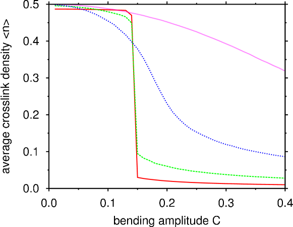
Figure 2: Behavior of the bundle upon bending. Plotted is the average crosslink density $\langle n\rangle$ versus bending amplitude $C$ for $k_{\times}/k_{\rm s}=10^{-5},10^{-4},10^{-3},10^{-2}$ (from top to bottom). For low values of $k_{\times}/k_{\rm s}$, $\langle n\rangle$ decreases smoothly with $C$; for higher values, a strong first-order transition is observed (data for $N_{\rm f}=2,N_{\times}=150,\mu=0$).

We begin our simulations with a bundle consisting of $N_{\rm f}=2$ filaments. In Fig. 2, we plot the average crosslink density $\langle n\rangle=\sum NP(N)/N_{\rm max}$, as function of the imposed bending amplitude $C$ for several values of $k_{\times}/k_{\rm s}$. In all cases, $\langle n\rangle$ decreases with $C$, showing that the crosslinks unbind upon bending. The striking feature is that, for $k_{\times}/k_{\rm s}$ high enough, $\langle n\rangle$ drops extremely sharply at some special value of the bending amplitude. In this situation, the unbinding of crosslinks is a collective phenomenon, reminiscent of a first-order phase transition.

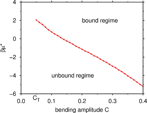
Figure 3: Phase diagram of a bundle consisting of $N_{\rm f}=2$ filaments. Plotted is the chemical potential $\mu^{\star}$ of the first-order transition versus the bending amplitude (data for $k_{\times}/k_{\rm s}=0.01,N_{\times}=300$).

We now specialize to $k_{\times}/k_{\rm s}=0.01$, i.e. the largest value considered in Fig. 2, where the transition is distinctly first-order. For a given bending amplitude $C$, we calculate the chemical potential $\mu^{\star}$ where the first-order transition occurs. To locate $\mu^{\star}$, $\mu$ is varied at fixed $C$ until the “susceptibility” $\chi=(\langle N^{2}\rangle-\langle N\rangle^{2})/N_{\rm max}$ reaches a maximum, i.e. we numerically solve

$$\mu^{\star}(C):\chi\to\mbox{max}.$$ (7)

The “phase diagram” of Fig. 3 shows $\mu^{\star}$ versus $C$ obtained in this way. This curve plays the role of a binodal: it separates the regime where the filaments are tightly bound by many crosslinks from the regime where they are only loosely coupled by few crosslinks. Note that the simulated binodal does not extend all the way $C\to 0$ but is “cut-off” at some threshold value $C=C_{T}$, which reflects the finite length of the bundle. Hence, $C_{T}$ does not correspond to a critical point in the usual thermodynamic sensetrivial2 .

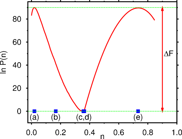
Figure 4: $\ln P(n)$ at $\mu^{\star}$ of the susceptibility maximum (conform Eq. (7)). The left (right) peak corresponds to an unbound (bound) bundle, while at intermediate densities the bundle is partially bound. Note the large free energy barrier $\Delta F$ separating the bound and unbound states (vertical arrow). The squares (a-e) indicate the densities $n$ at which the crosslink profiles of Fig. 5 were measured (data for $N_{\rm f}=2,N_{\times}=300,k_{\times}/k_{\rm s}=0.01,C=0.195$).

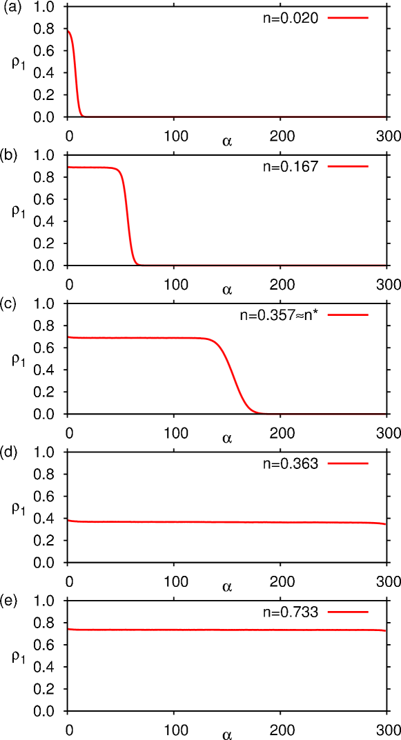
Figure 5: Crosslink density profiles $\rho_{1}(\alpha)$ for several values of the overall crosslink density $n$. The values of $n$ in (a,e) coincide with the peak positions in $P(n)$ of Fig. 4 and thus reflect the “coexisting” unbound and bound states. By increasing $n$, a domain wall gradually shifts toward the bundle center (b,c) up to a density $n^{\star}$ where it “jumps” to the bundle end (d). For the parameters used here $(N_{\rm f}=2,N_{\times}=300,k_{\times}/k_{\rm s}=0.01,C=0.195)$ we find $n^{\star}\approx 0.36$, which coincides with the crosslink density where $P(n)$ attains its minimum.

Next, we investigate how the crosslinks unbind at the transition (i.e. when $\mu=\mu^{\star}$). In Fig. 4, we show the logarithm of the distribution $P(n)$ measured at $\mu^{\star}$ (note that $\ln P(n)$ may be regarded as minus the free energy of the bundle). The distribution is distinctly bimodal, as is characteristic of a first-order transition citeulike:3717210 . In addition, we have checked that the barrier $\Delta F$ increases with the bundle length trivial3 , providing further confirmation that the transition is genuinely first-order citeulike:3908342 .

To understand how the transition from the unbound to the bound state progresses, we associate features of the distribution $P(n)$ to the spatial organization of crosslinks within the bundle. To this end, we introduce the crosslink density profile $\rho_{i}(\alpha)\equiv\langle n_{i,\alpha}\rangle$ measured along the bundle contour $\alpha=1,\ldots,N_{\times}$ between “adjacent” filaments $i$ and $i+1$. Of course, for $N_{\rm f}=2$, there is only one such profile: $\rho_{1}(\alpha)$. Some typical profiles are shown in Fig. 5, each obtained for a different value of the overall crosslink density $n$. In (a), we show $\rho_{1}(\alpha)$ for $n=0.020$, corresponding to the left peak in $P(n)$ where the bundle is unbound. We observe that $\rho_{1}(\alpha)>0$ only in a small region near the grafted end, but rapidly decays to zero thereafter. Hence, there is an interface (domain wall) in the system, separating a region of high crosslink density from one of low crosslink density. As $n$ increases, the domain wall gradually shifts toward the center of the bundle (b,c) up to some threshold density $n^{\star}$. At $n^{\star}$, the domain wall jumps discontinuously toward the bundle end, yielding a constant crosslink density along the entire contour (d). The value of $n^{\star}$ is given by the crosslink density where $P(n)$ attains its minimum. Once the domain wall has “jumped”, increasing $n$ further no longer affects the shape of the profile but merely raises the plateau value (e).

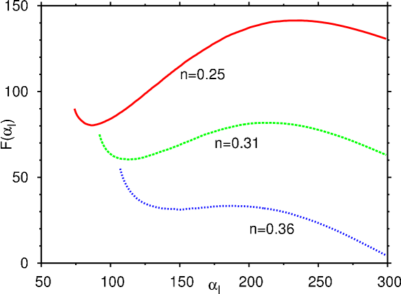
Figure 6: Bundle free energy $F(\alpha_{\rm I})$ as function of the domain wall position $\alpha_{\rm I}$ for three values of the crosslink density $n$. As $n$ increases, a first-order transition takes place at which the domain wall “jumps” from $\alpha_{\rm I}<N_{\times}/2$ to $\alpha_{\rm I}=N_{\times}$ (data for $N_{\rm f}=2,N_{\times}=300,k_{\times}/k_{\rm s}=0.01,C=0.195$).

The fact that the domain wall “jumps” at $n^{\star}$ indicates another first-order transition. To make this explicit, we performed a number of canonical simulations (i.e. at fixed $n$), and measured the bundle free energy $F(\alpha_{\rm I})$ as function of the domain wall position $\alpha_{\rm I}$ (in simulations $\alpha_{\rm I}$ is set by the crosslink furthest away from the grafted end). The result is shown in Fig. 6 for three values of the crosslink density $n$. In all cases, $F(\alpha_{\rm I})$ reveals two minima: the minimum at $\alpha_{\rm I}<N_{\times}/2$ ($\alpha_{\rm I}=N_{\times}$) corresponds to the unbound (bound) state. Note that the overall shape of $F(\alpha_{\rm I})$ rather resembles a cubic polynomial in $\alpha_{\rm I}$, which is the standard form of the Landau free energy expansion to describe a first-order transition ($\alpha_{\rm I}$ being the order parameter, and $n$ the temperature). For small $n$, the unbound state is stable (top curve). As $n$ increases, a first-order transition takes place above which the bound state is stable (lower curve). Precisely at the transition, the minima have the same free energy, here at $n\approx 0.31$ (center curve). Note that this somewhat underestimates $n^{\star}\approx 0.36$ of Fig. 5. One reason for the discrepancy is the use of different ensembles (canonical versus grand-canonical) in systems of finite size. Another reason is that the (un)bound states remain meta-stable over a considerable range in $n$ around the transition. To accurately obtain $n^{\star}$, one would need to perform an umbrella sampling simulation of the full two-dimensional probability distribution $P(N,\alpha_{\rm I})$.

III.2 The case $N_{\rm f}=4$

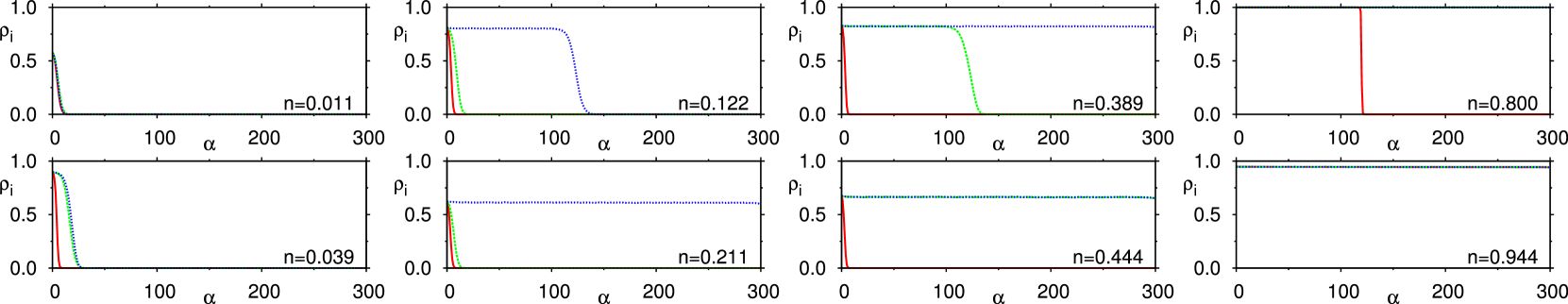
Figure 7: Simulation evidence for the existence of a sequence of binding/unbinding transitions in a bundle consisting of $N_{\rm f}=4$ filaments. Plotted are the crosslink density profiles $\rho_{i}(\alpha)$ for several values of the crosslink density $n$. In each of the graphs, the solid curve corresponds to $\rho_{2}(\alpha)$ of the center filament pair; dotted and dashed curves represent $\rho_{1}(\alpha)$ and $\rho_{3}(\alpha)$ of the outer pairs (data for $N_{\times}=300$, $k_{\times}/k_{\rm s}=0.01$, $C=0.19$).

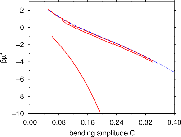
Figure 8: Phase diagram of a bundle consisting of $N_{\rm f}=4$ filaments (solid curves). Plotted is the chemical potential $\mu^{\star}_{I}$ of the $I=1,2,3$ first-order phase transitions versus the bending amplitude; the deep lower curve corresponds to the binding of the center filament pair (data for $k_{\times}/k_{\rm s}=0.01,N_{\times}=200$). For completeness, the binodal for $N_{\rm f}=2$ is also shown (dotted curve). As in Fig. 3, the binodals do not extend to $C\to 0$ due to finite bundle length.

More generally, for a bundle consisting of $N_{\rm f}$ filaments, we expect a sequence of $N_{\rm f}-1$ first-order transitions, one for each pair of adjacent filaments. To characterize these transitions, crosslink density profiles were measured for a bundle with $N_{\rm f}=4$. In this case, there are $i=1,2,3$ adjacent filament pairs, with corresponding density profiles $\rho_{i}(\alpha)$. The profiles are depicted in Fig. 7 for several values of the crosslink density $n$. For small $n$, the bundle is unbound: $\rho_{i}(\alpha)$ is zero everywhere, except for a small region near the grafted end ($n=0.011$). As $n$ increases, the crosslinks preferentially bind the outer filament pairs ($i=1,3$), while the center pair ($i=2$) remains unbound ($n=0.039$). Increasing $n$ further, the initial symmetry between outer pairs gets broken: with equal probability, one of the outer pairs $i=1,3$ is selected; the binding of crosslinks then continues for that pair only ($n=0.122$) ultimately leading to the first transition of the sequence ($n=0.211$). After the first transition, we thus have a bundle where one of the outer filament pairs is bound, while the remaining two pairs are unbound. Next, the other outer pair begins to bind ($n=0.389$) leading to the second transition ($n=0.444$). We now have a bundle where both outer filament pairs are bound, and the “$1\leftrightarrow 3$” symmetry is restored again. Not surprisingly, the third (and last) transition of the sequence involves the binding of the center filament pair. The mechanism is the same as before, featuring a domain wall ($n=0.800$) that “jumps” at the transition ($n=0.944$).

Note that the binding transitions of the outer filament pairs occur relatively close to each other (the corresponding densities are $n_{1}\sim 0.2$ and $n_{2}\sim 0.4\approx 2n_{1}$, respectively). However, to induce the binding of the center pair, a significantly larger density $n_{3}\sim 0.9$ is required. This becomes more pronounced in the $(C,\mu)$ phase diagram. To each transition $I=1,2,3$ in the sequence corresponds a (local) maximum in the susceptibility, and so the transition chemical potential $\mu^{\star}_{I}$ can be evaluated via Eq. (7) as before. The resulting phase diagram now features three binodals, with those corresponding to the binding of the outer filament occurring very close together (Fig. 8). Note also that the first of these “outer” binding transitions coincides with the binodal of the $N_{\rm f}=2$ bundle.

IV Theory

We now present a theoretical description that captures most of the features observed in the Monte Carlo simulations.

IV.1 The case $N_{\rm f}=2$ without bending

We first consider a two-filament bundle ($N_{\rm f}=2$) without external deformation ($C=0$). Assume all crosslinks to be bound for the moment, $n_{1,\alpha}=1$, with $\alpha=1,\ldots,N_{\times}$. The Hamiltonian of Eq. (6) then becomes

$$H_{\rm bundle}=\frac{\Gamma_{1}}{2}\Delta_{1}^{2}+\frac{1}{2}\sum_{\alpha=1}^{N_{\times}}\left[\frac{k_{\rm s}}{2}(\Delta_{\alpha+1}-\Delta_{\alpha})^{2}+k_{\times}\Delta_{\alpha}^{2}\right]\,,$$

with $\Delta_{\alpha}\equiv u_{2,\alpha}-u_{1,\alpha}$ and $\Gamma_{1}\equiv k_{\rm s}/2$. Strictly speaking, we also need to include the combination $\Sigma_{\alpha}\equiv u_{2,\alpha}+u_{1,\alpha}$. However, as the latter do not couple to the crosslink occupation variables, we need not consider them in our treatment.

The idea is to iteratively integrate out the degrees of freedom $\Delta_{\alpha}$, and to monitor the resulting “flow” of the coupling constant $\Gamma$. Each time one of the $\Delta_{\alpha}$ variables is integrated out, the Hamiltonian retains the above form, but with a renormalized coefficient $\Gamma$ given by the recursion relation

$$\Gamma_{i+1}=\frac{k_{\rm s}}{2}\frac{k_{\times}+\Gamma_{i}}{k_{\times}+k_{\rm s}/2+\Gamma_{i}}\,,$$ (8)

with the fixed-point

$$\Gamma_{\infty}=\frac{k_{\times}}{2}\left(\sqrt{1+2k_{\rm s}/k_{\times}}-1\right)\,.$$ (9)

At the $i$-th iteration step, the partition function $Z$ thus acquires a factor $(k_{\times}+k_{\rm s}/2+\Gamma_{i})^{-1/2}$, such that one can write

$$Z=e^{-\beta\mu N_{\times}}\prod_{i=1}^{N_{\times}}\left(\frac{\displaystyle k_{\times}+\Gamma_{i}}{\displaystyle\Gamma_{i+1}}\right)^{-1/2},$$ (10)

where we have used Eq. (8) and dropped an overall factor $(k_{\rm s}/2)^{-N_{\times}/2}$.

To see how the above generalizes to the case of open crosslinks let us assume that the crosslinks from sites $\alpha=j,\ldots,j+l_{j}-1$ are open. We will call this a “bubble” of length $l_{j}$ in the following. The associated variables $\Delta_{\alpha}$ can immediately be integrated over, with the effect of generating a term

$$(k_{\rm s}^{\rm eff}/2)(\Delta_{j+l_{j}}-\Delta_{j-1})^{2},\quad k_{\rm s}^{\rm eff}\equiv k_{\rm s}/(l_{j}+1),$$

in the renormalized Hamiltonian. Thus, to account for bubbles, we have to substitute the stretching stiffness $k_{\rm s}$ with $k_{\rm s}^{\rm eff}$ in Eqs. (8) and (10), as well as to reinterpret $N_{\times}$ as the number of bound sites: $N_{\rm bound}\equiv N$. The resulting expression is an exact, albeit intractable, representation of the partition function.

To make progress, we use a mean-field (MF) approximation, where we assume the crosslinks to be homogeneously distributed along the bundle (the interface will be accounted for later). The actual bubble length thus gets replaced by its average value $1/(l_{j}+1)\to N/N_{\times}\equiv x$, where $x$ denotes the fraction of bound crosslinks. Furthermore, we replace the renormalized coupling constant by its fixed-point value, $\Gamma_{i}\to\Gamma_{\infty}$, which in our MF approximation can be written as

$$\Gamma_{\infty}(x)=\frac{k_{\times}}{2}\left(\sqrt{1+2xk_{\rm s}/k_{\times}}-1\right).$$

Within these approximations, the partition function of Eq. (10) evaluates to

$$Z_{\rm MF}=\sum_{N=0}^{N_{\times}}p_{N}\,e^{-\beta\mu N}\left(1+\frac{k_{\times}}{\Gamma_{\infty}(N/N_{\times})}\right)^{-N/2}\,,$$ (11)

which can easily be evaluated numerically. The term $p_{N}=\binom{N_{\times}}{N}$ represents the usual “entropy of mixing” and counts the number of crosslink configurations compatible with a given $N=xN_{\times}$. We will show in Appendix B how the averaged crosslink occupation $\langle n\rangle$ compares to our simulation results. We will furthermore show how one can improve the theory by explicitly incorporating bubbles using the “necklace model” of Fisher  fisherJStatPhys1984Necklace ; husePRB1984Necklace .

IV.2 The case $N_{\rm f}=2$ with bending and interface

Next, we incorporate a finite bending amplitude $\theta_{\alpha}$ into the theory. In addition, as the simulations indicate the possibility of an interface between a region of high and low crosslink density, we must appropriately generalize the above MF approach to the crosslink occupation variables $n_{1,\alpha}$. To this end, we assume the crosslinks to be homogeneously distributed in the region of high density only. A sharp interface separates this region from one without crosslinks

$$n_{1,\alpha}=\begin{cases}xN_{\times}/\alpha_{\rm I}&\alpha<\alpha_{\rm I},\\ 0&\alpha>\alpha_{\rm I},\end{cases}$$ (12)

where $\alpha_{\rm I}\in[0,N_{\times}]$ is the (unknown) axial position of the interface. Below we will also use the normalized interface position

$$y=\alpha_{\rm I}/N_{\times}\in[0,1]\,.$$ (13)

As before, $x$ denotes the fraction of bound crosslinks, which can be expressed in terms of the occupation variables as $x=\sum_{\alpha}n_{1,\alpha}/N_{\times}$.

We now make an “Ansatz” for the displacement degrees of freedom $u_{i,\alpha}$. We assume that the quadratic terms in Eq. (5) are small whenever there are crosslinks that bind the two filaments together. That is, provided $n_{1,\alpha}=1$, the corresponding displacement $\Delta_{\alpha}\equiv u_{2,\alpha}-u_{1,\alpha}\propto\theta_{\alpha}$. In the region of low crosslink density we can assume that $\Delta_{\alpha}=\rm const$. We thus obtain

$$\Delta_{\alpha}=\begin{cases}u_{0}\sin(\pi\alpha/2N_{\times})&\alpha<\alpha_{\rm I},\\ u_{0}\sin(\pi\alpha_{\rm I}/2N_{\times})&\alpha>\alpha_{\rm I},\end{cases}$$ (14)

by requiring continuity at $\alpha=\alpha_{\rm I}$, and where also Eq. (4) was used. Introducing these expressions into the Hamiltonian of Eq. (6), and minimizing with respect to $u_{0}$, we obtain the following “saddle-point” contribution to the effective free energy

$$F_{\rm sp}(x,y)=N_{\times}Af_{c}(y)\left[1+\displaystyle\frac{x_{0}}{x}\cdot\frac{yf_{c}(y)}{f_{s}(y)}\right]^{-1}\,,$$ (15)

with functions

$$\begin{split}f_{c}(y)=\frac{2}{L}\int_{0}^{yL}\cos^{2}(\pi s/2)L\,ds\,,\\ f_{s}(y)=\frac{2}{L}\int_{0}^{yL}\sin^{2}(\pi s/2L)\,ds\,,\end{split}$$ (16)

and bundle length $L=aN_{\times}$. The relevant parameters are $A\simeq k_{\rm s}b^{2}(Ca)^{2}$, which encodes the dependence on bending amplitude $A\propto C^{2}$, and $x_{0}\simeq(k_{s}/k_{\times})/N_{\times}^{2}$ representing the effects of the crosslink stiffness $x_{0}\propto 1/k_{\times}$. The point to note is that $F_{\rm sp}(x,y)$ still depends on the crosslink occupation variable $x$, as well as on the location of the interface $\alpha_{\rm I}$ (via the parameter $y$ of Eq. (13)).

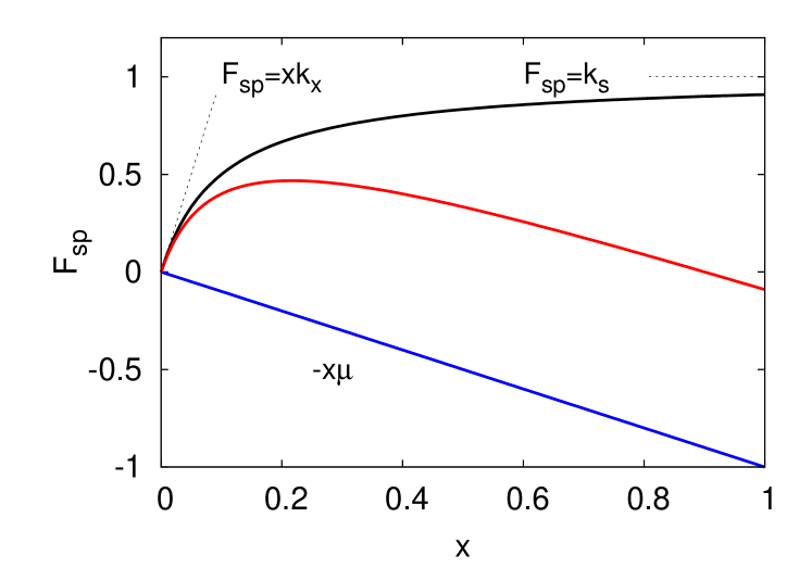
Figure 9: Illustration of the mechanism that induces a discontinuous reduction of the crosslink occupation as function of bending amplitude and/or chemical potential. The top curve shows $F_{\rm sp}(x)$ of Eq. (17), with the dashed lines indicating the limiting behaviors for $x\to 0$ and $x\to 1$. The binding enthalpy $-x\mu$ (lower line), which is to be added to $F_{\rm sp}(x)$, “tilts” the free energy landscape, leading to a free energy (center curve) featuring a coexistence between two states (at high and low crosslink occupation $x$, respectively). As the control parameters $A,\mu$ are varied, a discontinuous transition from one state to the other is thus observed.

In a previous report PhysRevE.83.050902 we presented the special case $y=1$, i.e. without an interface being present. In this limit one obtains for the free energy

$$F_{\rm sp}(x,y=1)\equiv F_{\rm sp}(x)=N\frac{A}{1+x_{0}/x}\,.$$ (17)

This simple form, which is illustrated in Fig. 9, conveys an intuitive picture of how a finite bending amplitude may lead to a discontinuous reduction of crosslink occupation $x$. When $x\ll x_{0}$ the free energy essentially grows linearly, $F_{\rm sp}(x)\sim xk_{\times}$, with the energy scale set by the crosslink stiffness $k_{\times}$. This indicates that each crosslink contributes a certain amount of deformation energy, while the filaments remain nearly undeformed. The few crosslinks present are just not strong enough to force the filaments into a deformed state. This situation changes when $x\gg x_{0}$, where the free energy saturates at a value set by the filament stretching stiffness, $F_{\rm sp}(x)\sim k_{\rm s}$. Now there are enough crosslinks to stretch out the filaments, at the same time relieving their own deformation. Together with the binding enthalpy, $E=-x\mu$, which leads to the usual tilting of the free energy landscape, we obtain a total free energy that has two coexisting states, at high and low crosslink occupation. As the bending amplitude $A$ or the chemical potential $\mu$ is varied, it is therefore possible to observe a discontinuous transition from one state to the other.

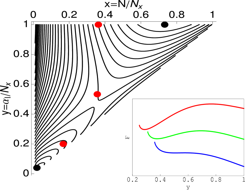
Figure 10: Contour plot of the total free energy $F(x,y)$ given by Eq. (18). Note that only the region $x<y$ is physically relevant as the total number of crosslinks $N$ is always less than $\alpha_{I}$. The dots correspond to the state points (a-e) in Fig. 5 where the crosslink profiles were obtained in simulations. The inset shows the free energy $F$ as function of the normalized interface position $y$ for fixed $x=0.25,0.31,0.36$ (from top to bottom), which compares well to the simulation result of Fig. 6.

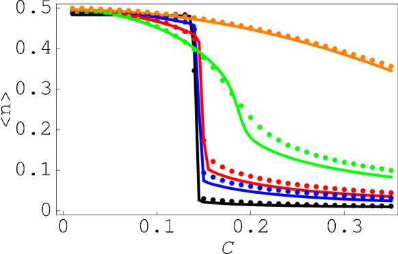
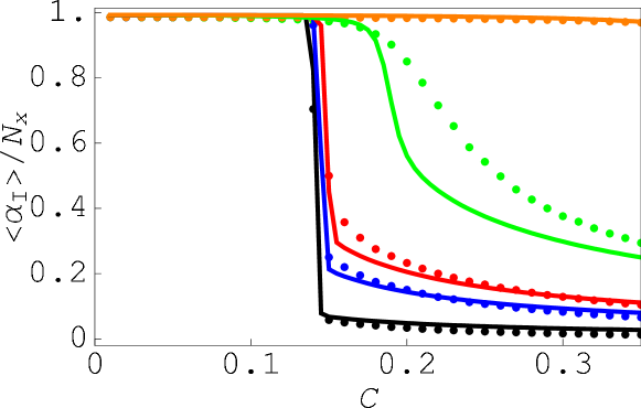
Figure 11: (top) Average crosslink occupation $\langle n\rangle$ and (bottom) average interface location $\langle\alpha_{\rm I}\rangle$ as function of bundle curvature $C$ using $N_{\times}=150$, and for different crosslink stiffness $k_{\times}/k_{\rm s}=10^{-5},10^{-4},4\cdot 10^{-4},10^{-3},10^{-2}$ (from top to bottom). In both graphs, the lines are obtained without fit parameters from the theoretical model, Eq. (18), while the symbols indicate simulation data.

The existence of an interface does not change fundamentally this picture but adds a second reaction coordinate that the bundle can utilize in order to minimize its free energy during the unbinding process. Combining Eqs. (11) and (15) we obtain $Z=\sum_{\alpha_{\rm I}=0}^{N_{\times}}\sum_{N=0}^{\alpha_{\rm I}}e^{-\beta F(N,\alpha_{\rm I})}$ with

$$e^{-\beta F(N,\alpha_{\rm I})} =$$ (18)

$$\left({\alpha_{\rm I}\atop N}\right) \times \left(1+\frac{k_{\times}}{\Gamma_{\infty}(N/\alpha_{\rm I})}\right)^{-N/2}\times e^{-\beta\left(F_{\rm sp}+\mu N\right)},$$

which defines the total free energy $F(N,\alpha_{\rm I})$. The latter is illustrated in Fig. 10 using parameters that correspond to the discontinuous transition of Fig. 5. The figure strikingly shows the coexisting states at high and low crosslink density, and the formation of an interface upon passing over the intermediate saddle-point. The theory also reproduces the free energy barrier along lines of constant $N$ (inset), in line with the canonical simulations of Fig. 6. The transition pathway followed in these simulations is indicated by the light (red) points. After passing the saddle-point, at $x\approx 0.35$, the interface “jumps” from the center of the bundle to the distant end. It is interesting to compare this “canonical” pathway with the general shape of the basin of attraction into the bound state. This seems to favor a pathway closer to the diagonal, with an associated continuous motion of the interface.

From Eq. (18) it is straightforward to calculate the average crosslink density $\langle n\rangle$, as well as the average location of the interface $\langle\alpha_{\rm I}\rangle$. Both are compared to simulation results in Fig. 11, and the agreement is remarkably good: as the bending amplitude increases, there is a discontinuous jump in both the crosslink density, as well as in the interface position.

IV.3 The case $N_{\rm f}>2$

Let us now turn to bundles with more than two filaments. The simulations have indicated a sequence of $N_{\rm f}-1$ transitions, one transition for each adjacent filament pair (Fig. 7). Upon increasing the bundle deformation $C$, the crosslinks in the central filament pair unbind first. This unbinding transition leaves two smaller weakly coupled sub-bundles. The successive transitions then happen in the centers of these sub-bundles up until all filament pairs are unbound.

As with each filament pair the number of variational parameters increases, a full theoretical treatment becomes intractable. We therefore choose a semi-analytic treatment that explicitly accounts for crosslinks in the respective central layer only. The stretching degrees of freedom that do not belong to this layer are integrated out by assumingheussingerPRE2010

$$u_{i+1,\alpha}-u_{i,\alpha}=\Delta_{\alpha}\,,$$ (19)

independent of the layer index $i$. This indicates that filament stretching increases approximately linearly with the filament index, i.e. with the distance from the center of the bundle (filaments farther out from the center “inherit” the stretching from all the filaments on the inside). Such a linear dependence constitutes a central assumption in classical continuum theories, such as Euler-Bernoulli or Timoshenko beam theories timoshenko . For sufficiently stiff crosslinks, and without considering the possibility of an interface ($y=1$), this model can be mapped onto a two-filament bundle, conform Eq. (17), with effective $N_{\rm f}$-dependent parameters, $A(N_{\rm f})\sim N_{\rm f}^{3}$ and $x_{0}(N_{\rm f})\sim N_{\rm f}$. We then use these $N_{\rm f}$-dependent parameters in the full free energy of Eq. (18) to calculate the average crosslink density for the given layer.

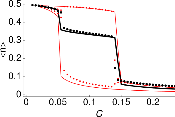
Figure 12: The analogue of Fig. 2 but for $N_{\rm f}=4$. The key difference is that we now observe a sequence of unbinding transitions. Plotted is the average crosslink density $\langle n\rangle$ as function of the bending amplitude $C$ for $k_{\times}/k_{\rm s}=10^{-3},\,\mu=0,\,N_{\times}=150$ (curves show results obtained using the “Ansatz” Eq. (19); symbols represent simulation data). The lower (upper) curve shows the crosslink density in the central (outer) layer. The middle curve reflects the crosslink density of the entire bundle, which was obtained by adding the contributions from the individual layers.

Fig. 12 compares the result of this calculation (curves) with simulation data (symbols) for the case $N_{\rm f}=4$. The middle curve shows the average crosslink density $\langle n\rangle$ of the entire bundle versus bending amplitude $C$: the agreement with the simulations is quite remarkable. The lower curve shows the average crosslink density in the central layer, which unbinds at $C\approx 0.05$. Here, the theory slightly underestimates the simulation results, but the location of the transition is accurately reproduced. The upper curve shows $\langle n\rangle$ of the outer layer, which unbinds at a much larger bending amplitude $C\approx 0.15$. This curve is nearly equivalent to that of a bundle with $N_{\rm f}=2$ filaments, in agreement with the binodal of Fig. 8.

V Discussion

We have studied the response of a reversibly crosslinked filament bundle to an imposed bundle deformation. The central quantity was the average crosslink density $\langle n\rangle$ and its dependence on the imposed curvature $C$ of the bundle backbone. As compared to simple Langmuir adsorption, $\langle n\rangle=1/(1+e^{\beta\mu})$ at chemical potential $\mu$, one expects a decreasing crosslink occupation with increasing bundle deformation. The reason is that bundle deformation leads to a mismatch between the crosslink binding sites, and therefore to an elastic energy cost for binding. We found this basic mechanism to indeed be true, but the detailed phenomenology of crosslink unbinding turns out to be surprisingly rich and goes beyond a simple shift of the equilibrium state as would be characterized, for example, by an effective chemical potential.

Our main result is the possibility of a cooperative and discontinuous reduction of crosslink occupation as the bundle deformation is increased. The reason for this behavior is the competition between the energy scales of crosslink shear $k_{\times}$, and filament stretch $k_{\rm s}$, which is particularly efficient when the crosslinks are stiff. An unbinding event will then affect the force balance in the filaments, with the potential of influencing the bundle state far away from the unbinding site. On the other hand, when $k_{\times}$ is small and the crosslinks soft, crosslinks unbind one after the other leading to a smooth decrease of the average crosslink occupation.

We have characterized in detail the discontinuous unbinding transition and identified the existence of an interface; the latter separates a region of high crosslink density from a region essentially free of crosslinks. The formation of an interface is a collective process in which crosslinks have to reorganize within the bundle and find new binding sites. A similar effect has been discussed in the context of the twisting of helical filament bundles, where crosslinks organize into certain “binding zones” heussingerJCP2011 . As one increases the bundle twist away from its preferred value, these binding zones become shorter and shorter, thus necessitating collective reorganizations of many crosslinks simultaneously. As evidenced in Fig. 6, such a process implies the crossing of a free energy barrier. The associated time-scale of escape over the barrier may be much longer compared to single crosslink (un)binding events.

Such long time-scales may indeed be present in a recent experiment with F-actin bundles crosslinked by $\alpha$-actininstrehleEBPJ2011 . In the experiment a bundle was brought into a deformed configuration, where it was kept for either ten or $1000$ seconds. After this waiting time the bundle was released and its relaxation was monitored. For the shorter waiting time the bundle showed the expected exponential relaxation into the straight ground state. For the longer waiting time, however, the bundle did not relax back, but remained in a state with a considerable residual bending deformation. Apparently, upon bundle deformation, new binding sites become available that stabilize the bent shape by allowing the crosslinks to rebind in more favorable states that avoid crosslink straining. After releasing the bundle these crosslinks act to stabilize the bent contour, thus leading to a plastically deformed bundle, where the ground-state is no longer straighttrivial5 . In line with our interpretation in terms of a free energy barrier, the apparent time-scale (the waiting time) necessary to observe bundle plasticity was considerably longer than the time required for (un)binding of the individual $\alpha$-actinin linkers, which is on the order of secondsWachsstockBPJ1993 .

Strictly speaking, our model does not allow for plastic deformation as the crosslinks are assumed to always bind to the same, initial binding sites: a crosslink at site $\alpha$ only binds to the site $\alpha$ on the next filament. We explicitly exclude the binding of crosslinks between non-neighboring sites, e.g. between $\alpha$ and $\alpha\pm 1$. If the bending-induced mismatch, $b\theta_{\alpha}$, between the original sites at $\alpha$ is large, those “new” sites may actually be more favorable in terms of crosslink energy. Binding to new sites may then help to “freeze-in” the applied bending deformation leading to a plastically deformed contour. Such a model would pose a challenging problem for a theoretical analysis and has to be left for future work. Instead, we propose a simple mapping that allows us to incorporate bundle plasticity into the “elastic” bundle model presented in this work.

To this end, we assume the new binding sites to be optimal, in the sense that for the given imposed bundle contour no elastic energy cost is associated with the rebinding of a crosslink. Reshuffling a crosslink from its original position to a new site may then be conceived of as being an unbinding event at zero chemical potential. For simplicity, we further assume that rebinding is fast enough, such that all crosslinks are either bound to original sites or to new sites. In this case, the number of crosslinks bound to new sites, $M$, can be inferred without further calculation from the results presented in this work, $\langle M\rangle=N_{\rm max}-\langle N\rangle_{\mu=0}$. If we now release the bundle from its deformed state, filament elasticity will try to relax the bundle back to its original unbent state. The population of newly bound crosslinks, however, acts against this relaxation and stabilizes the bent contour. Within our assumption the additional contribution to the crosslink shear energy is

$$H^{\rm new}_{\times}=\frac{k_{\times}M}{2N_{\times}}\sum_{\alpha=1}^{N_{\times}}\left(\Delta_{\alpha}+b(\theta_{\alpha}-\theta_{\alpha}^{0})\right)^{2}\,,$$ (20)

where we assumed $N_{\rm f}=2$ for simplicity. Here, $\theta_{\alpha}^{0}$ is the tangent in the reference configuration at position $\alpha$ that was imposed during the waiting time, while $\theta_{\alpha}$ corresponds to the tangent acquired during the relaxation process.

As can be seen, the magnitude of the stabilizing effect depends on $M$, which depends on the waiting time. If the crosslink is stiff enough, such that a free energy barrier is present, fast thermalization is prevented. In this case $M\approx 0$ on short time-scales and the bundle will behave elastically. On time-scales long compared to the escape time over the barrier, the number of crosslinks bound to new sites reaches its equilibrium value, $M=\langle M\rangle$, and the bundle is maximally plastic. In the experiment of Ref. strehleEBPJ2011, only two waiting times were accessible. It would be interesting to systematically change the experimental time-scale. One possibility could be to introduce a rate, at which bundle deformation is increased. In the context of protein unfolding, similar experimentsdudkoPNAS2008 have proved extremely useful to extract information on the underlying free energy landscape.

Appendix A Monte Carlo method

The bundle is represented by a two-dimensional $(i=1,\ldots,N_{\rm f})\times(\alpha=1,\ldots,N_{\times})$ lattice. To each lattice site $(i,\alpha)$ a real number $u_{i,\alpha}$ is attached, denoting the local axial displacement. In addition, occupation variables $n_{i,\alpha}=(0,1)$ are attached to “vertical” nearest neighboring pairs $(i,\alpha)$ and $(i+1,\alpha)$. We simulate in the grand canonical ensemble using a biased Hamiltonian

$$H_{\rm bias}=H_{\rm bundle}+W(N),$$ (21)

with $H_{\rm bundle}$ the “unbiased” Hamiltonian of Eq. (6), and $W(N)$ a weight function defined on the total number of crosslinks $N$. The purpose of $W(N)$ is to sample all microstates $0\leq N\leq N_{\rm max}$ with equal probability. To construct $W(N)$, which is a priori unknown, we use successive umbrella sampling virnau.muller:2004 . Once known, the sought-for probability distribution in the number of crosslinks follows as $P(N)\propto\exp(-\beta W(N))$. As Monte Carlo moves we use single bead displacements and crosslink binding/unbinding moves, each attempted with equal probability. In a displacement move, a lattice site $(i,\alpha)$ is selected randomly, and the current displacement $u_{i,\alpha}$ of that site is replaced by $u_{i,\alpha}^{\prime}=u_{i,\alpha}+\delta$, with $-0.1<\delta<0.1$ drawn uniformly randomly. The new displacement $u_{i,\alpha}^{\prime}$ is accepted with probability $P_{\rm disp}=\min\left[1,e^{-\beta\Delta H}\right]$, where $\Delta H$ is the energy difference between initial and final state (since displacements do not change $N$, both Eq. (6) and Eq. (21) can be used to compute the energy difference). During a crosslink move, a vertical bond is selected randomly, and the corresponding occupation variable $n_{i,\alpha}$ is “flipped” ($n_{i,\alpha}=0$ gets replaced by 1, and vice versa). The new state is accepted with probability $P_{\rm xlink}=\min\left[1,e^{-\beta\Delta H_{\rm bias}+\beta\mu\Delta N}\right]$, with $\mu$ the crosslink chemical potential, $\Delta N=\pm 1$ the change in the number of crosslinks, and $\Delta H_{\rm bias}$ the energy difference which must now be calculated using the biased Hamiltonian of Eq. (21).

Appendix B Comparison to simple mean-field
theory and the necklace model

The simple mean-field approximation developed in Eq. (11) is capable of accurately describing the thermodynamic properties of the bundle without external deformation, i.e. $C=0$. One can slightly improve on this result by explicitly incorporating the bubbles along the lines of the classic “necklace model” fisherJStatPhys1984Necklace ; husePRB1984Necklace .

The partition function for a bubble of length $M$ is obtained from Eqs. (8) and (10) by setting $k_{\times}=\mu=0$

$$Z_{0}(M)=\prod_{i=1}^{M}(k_{s}/2+\Gamma_{i})^{-1/2}=(1+\frac{M}{M_{c}})^{-1/2}\,,$$ (22)

where we defined a characteristic bubble size $M_{c}=k_{s}/2\Gamma_{0}$. The value of the coupling constant at the beginning of the bubble, $\Gamma_{0}$, can be taken equal to the fixed-point value in the neighboring bound segment, $\Gamma_{0}=\Gamma_{\infty}(k_{\times})$. The partition function of a bound segment of length $N$ is

$$Z_{1}(N)=\left[e^{-\beta\mu}\left(1+\frac{k_{\times}}{k_{\infty}}\right)^{-1/2}\right]^{N}\,.$$ (23)

The full partition function can be obtained from the generating functions $\Phi_{\alpha}(z)=\sum_{N=1}^{\infty}z^{N}Z_{\alpha}(N)$ and the solution to the equation $\Phi_{0}(z)\Phi_{1}(z)=1$. From this the average crosslink density $\langle n\rangle$ is obtained in the usual way by differentiating with respect to $\mu$. The quality of the different approximations is compared in Fig. 13.

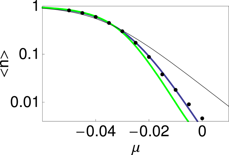
Figure 13: Average crosslink density $\langle n\rangle$ of an undeformed bundle ($C=0$) consisting of $N_{\rm f}=2$ filaments as function of the chemical potential $\mu$ using $k_{\times}/k_{\rm s}=10^{-3},N_{\times}=100$. Note the logarithmic vertical scale! The thin curve is the solution of the one-crosslink model, as presented by Eq. (5) of Ref. PhysRevE.83.050902, , while the thick curves were calculated using Eq. (11) (lower curve) and the necklace model (middle curve). The latter indeed yields better agreement with the simulation results (dots).