Dark matter and LHC phenomenology in a left-right supersymmetric model

Abstract

Left-right symmetric extensions of the Minimal Supersymmetric Standard Model can explain neutrino data and have potentially interesting phenomenology beyond that found in minimal SUSY seesaw models. Here we study a SUSY model in which the left-right symmetry is broken by triplets at a high scale, but significantly below the GUT scale. Sparticle spectra in this model differ from the usual constrained MSSM expectations and these changes affect the relic abundance of the lightest neutralino. We discuss changes for the standard stau (and stop) co-annihilation, the Higgs funnel and the focus point regions. The model has potentially large lepton flavour violation in both, left and right, scalar leptons and thus allows, in principle, also for flavoured co-annihilation. We also discuss lepton flavour signals due to violating decays of the second lightest neutralino at the LHC, which can be as large as $20$ fb^-1 at $\sqrt{s}=14$ TeV.

I Introduction

Left-right (LR) symmetric extensions of the MSSM (“Minimal Supersymmetric extension of the Standard Model”) automatically contain the correct ingredients to explain the observed neutrino masses and mixings. The right-handed neutrino superfield, $\nu^{c}$, is necessarily part of the theory and breaking the LR symmetry by $SU(2)_{R}$ triplets generates at the same time a Majorana mass term for the $\nu^{c}$ and thus a seesaw mechanism Minkowski:1977sc ; MohSen ; Schechter:1980gr ; Cheng:1980qt , in contrast to type-I seesaw models where a Majorana mass term is merely added by hand. In LR models new gauge and Higgs fields appear with masses below the GUT scale, which change the running of all parameters under RGE evolution. In particular, the change in the running of the soft supersymmetry breaking masses can lead to potentially interesting effects in the phenomenology of SUSY models, even if the scale of LR breaking is above the energy range testable by accelerator experiments.

Quite a large number of different LR models have been discussed in the literature. The original (non-supersymmetric) LR models Pati:1974yy ; Mohapatra:1974gc ; Senjanovic:1975rk break the $SU(3)_{C}\times SU(2)_{L}\times SU(2)_{R}\times U(1)_{B-L}$ group by scalar doublets. Later it was realized that breaking the LR symmetry by (a pair of) triplets with $B-L=2$ generates automatically also a seesaw mechanism MohSen ; Mohapatra:1980yp . Four triplets are needed Cvetic:1983su in the supersymmetric version of this LR model: $\Delta(1,3,1,2)$ and $\Delta^{c}(1,1,3,-2)$ due to the LR symmetry and $\bar{\Delta}(1,3,1,-2)$ and $\bar{\Delta}^{c}(1,1,3,2)$ for anomaly cancellation. Aulakh et al. Aulakh:1997ba ; Aulakh:1997fq extended this minimal LR model introducing an additional pair of triplets $\Omega(1,3,1,0)$ and $\Omega^{c}(1,1,3,0)$ with zero lepton number. The advantages of this setup, in the following called the $\Omega$LR model, are two-fold Aulakh:1997fq : First, the LR breaking minimum leaves R-parity unbroken already at tree level and, second, a non-trivial CKM matrix for quarks is generated easily and without resorting to flavour violating soft terms Babu:1998tm .

Both, the minimal SUSY LR model Cvetic:1983su as well as the $\Omega$LR model Aulakh:1997ba ; Aulakh:1997fq break the LR symmetry at an energy scale far above the range accessible to accelerator experiments. Only indirect tests of these models are therefore possible, all of which require some assumptions about the high scale boundary conditions for the soft SUSY breaking terms. Assuming CMSSM (“constrained” MSSM) Drees:2004jm boundary conditions, two kind of indirect signals are possible, in principle: (i) Lepton flavor violating (LFV) decays and (ii) changes in the SUSY particle mass spectra.

LFV decays are induced in supersymmetric models, even for strictly flavour blind boundary conditions, in the RGE running of the soft parameters, as has been shown for the case of type-I seesaw already in Borzumati:1986qx . With LFV observed in neutrino oscillation experiments Fukuda:1998mi , one expects LFV to occur also in the charged lepton sector in practically all SUSY models. However, there is a qualitative difference between seesaw models and LR models: whereas in SUSY seesaw LFV is expected to occur dominantly in the left slepton sector Hisano:1995nq ; Hisano:1995cp , an LR symmetry implies that left and right sleptons should have equal soft mass terms. Even with LR symmetry then broken at low energies, LFV in the right slepton sector can be sizable, as was shown in Esteves:2010si . Right slepton LFV could, in principle, be detected directly at accelerators or indirectly by measuring polarization in the decay $\mu\to e\gamma$ Kuno:1999jp .

Potentially measurable differences in SUSY mass spectra with respect to CMSSM expectations can occur in seesaw type-II Hirsch:2008gh ; Hirsch:2011cw and type-III Hirsch:2011cw ; Esteves:2010ff , as well as in the $\Omega$LR model Esteves:2010si . Changes with respect to CMSSM can best be understood analytically by forming certain “invariants”, i.e. soft SUSY breaking mass parameter combinations which are to 1-loop leading-log order constants over large ranges in CMSSM space Buckley:2006nv . Although there are quantitatively important 2-loop corrections to these invariants, as we will show below in the $\Omega$LR model the invariants have qualitatively different behavior from all seesaw models, due to the LR symmetry. This is similar to the situation discussed recently in DeRomeri:2011ie in the context of different $SO(10)$ based models.

Even slight changes in the SUSY spectra can lead to rather sizable changes in the calculated relic density of the lightest neutralino, $\Omega_{\tilde{\chi}^{0}_{1}}h^{2}$, as has been shown for seesaw type-II Esteves:2009qr and type-III Esteves:2010ff ; Biggio:2010me and also for an SO(10) based model Drees:2008tc . This fact can be easily understood taking into account that all solutions in CMSSM parameter space Drees:1992am , which survive the latest WMAP constraints Komatsu:2010fb , require some special relations among SUSY masses in order to get a low enough $\Omega_{\tilde{\chi}^{0}_{1}}h^{2}$. For example, in the stau co-annihilation region $\Omega_{\tilde{\chi}^{0}_{1}}h^{2}$ is essentially determined by $\Delta m=m_{\tilde{\tau}_{1}}-m_{\tilde{\chi}^{0}_{1}}$, as long as $\Delta m\raise 1.29167pt\hbox{$\;<$\kern-7.5pt\raise-4.73611pt\hbox{$\sim\;$}}10$ GeV or so. Changing $m_{\tilde{\tau}_{1}}$ and/or $m_{\tilde{\chi}^{0}_{1}}$ by only a few GeV will then change $\Omega_{\tilde{\chi}^{0}_{1}}h^{2}$ by a large factor. Below we will discuss how the standard solutions to the DM problem are changed within the $\Omega$LR, with respect to the “pure” CMSSM allowed regions. Since the $\Omega$LR model has potentially large LFV in the right slepton sector, the DM constraint can also be fulfilled using the flavoured co-annihilation solution, recently discussed in Choudhury:2011um . We provide and discuss a few examples where flavoured co-annihilation can be realized in the parameter space of the $\Omega$LR model.

Finally, LFV SUSY decays might be seen at the LHC. In Esteves:2010si we have shown that branching ratios $\tilde{\chi}^{0}_{2}\to l_{i}l_{j}\tilde{\chi}^{0}_{1}$, with $i\neq j$ are potentially large within the $\Omega$LR. Here we extend this work by calculating the SUSY production cross section for $\tilde{\chi}^{0}_{2}$ from cascade decays, to estimate the number of events that could be found at the LHC. We have found $\sigma\times Br(\tilde{\chi}^{0}_{2}\to l_{i}l_{j}\tilde{\chi}^{0}_{1})$ up to $(10-20)$ $fb$.

The rest of this paper is organized as follows. In the next section, we define the basics of the $\Omega$LR model. In section III we discuss gauge coupling unification, generalities for the expected changes in the SUSY spectra with respect to CMSSM expectations and certain aspects of lepton flavour violation. In section IV we discuss dark matter in the $\Omega$LR model, while section V discusses lepton flavour violation phenomenology for the LHC. We then close with a short summary.

II Model

In this section we present the model originally defined in Aulakh:1997ba ; Aulakh:1997fq , where a two step breaking of the LR symmetry was proposed in order to cure the potential problems related to the conservation of R-parity at low energies Kuchimanchi:1993jg ; Kuchimanchi:1995vk . For further details see Esteves:2010si .

II.0.1 Step 1: From GUT scale to $SU(2)_{R}$ breaking scale

Below the GUT scale the gauge group of the model is $SU(3)_{c}\times SU(2)_{L}\times SU(2)_{R}\times U(1)_{B-L}$. In addition, parity is assumed to be conserved. Besides the quark and lepton superfields of the MSSM with the addition of (three) right-handed neutrino(s) $\nu^{c}$, some additional superfields are required to break the LR symmetry down to the standard model gauge group. First, two generations of $\Phi$ superfields, bidoublets under $SU(2)_{L}\times SU(2)_{R}$, are introduced. They contain the standard $H_{d}$ and $H_{u}$ MSSM Higgs doublets. Note, that two copies are needed in order to generate a non-trivial CKM matrix at tree-level. Furthermore, triplets under (one of) the $SU(2)$ gauge groups are added whose gauge quantum number are given in Table 1. Note that the model contains $B-L=\pm 2$ and $B-L=0$ triplets.

With these representations, the most general superpotential compatible with the symmetries is

$${\cal W} = Y_{Q}Q\Phi Q^{c}+Y_{L}L\Phi L^{c}-\frac{\mu}{2}\Phi\Phi+fL\Delta L+f^{*}L^{c}\Delta^{c}L^{c}$$ (1)

$$+ a\Delta\Omega\bar{\Delta}+a^{*}\Delta^{c}\Omega^{c}\bar{\Delta}^{c}+\alpha\Omega\Phi\Phi+\alpha^{*}\Omega^{c}\Phi\Phi$$

$$+ M_{\Delta}\Delta\bar{\Delta}+M_{\Delta}^{*}\Delta^{c}\bar{\Delta}^{c}+M_{\Omega}\Omega\Omega+M_{\Omega}^{*}\Omega^{c}\Omega^{c}\thickspace.$$

Note that the superpotential in eq. (1) is invariant under the parity transformations $Q\leftrightarrow(Q^{c})^{*}$, $L\leftrightarrow(L^{c})^{*}$, $\Phi\leftrightarrow\Phi^{\dagger}$, $\Delta\leftrightarrow(\Delta^{c})^{*}$, $\bar{\Delta}\leftrightarrow(\bar{\Delta}^{c})^{*}$, $\Omega\leftrightarrow(\Omega^{c})^{*}$. This discrete symmetry fixes, for example, the $L^{c}\Delta^{c}L^{c}$ coupling to be $f^{*}$, the complex conjugate of the $L\Delta L$ coupling, thus reducing the number of free parameters of the model.

Superfield	$SU(3)_{c}$	$SU(2)_{L}$	$SU(2)_{R}$	$U(1)_{B-L}$
$\Delta$	1	3	1	2
$\bar{\Delta}$	1	3	1	-2
$\Delta^{c}$	1	1	3	-2
$\bar{\Delta}^{c}$	1	1	3	2
$\Omega$	1	3	1	0
$\Omega^{c}$	1	1	3	0

Table 1: Summary of the triplets of the $\Omega$LR model above the $SU(2)_{R}$ breaking scale.

Family and gauge indices have been omitted in eq. (1), more detailed expressions can be found in Aulakh:1997ba . Moreover, the soft terms of the model can be found in Esteves:2010si . The LR symmetry itself does not, of course, fix the values of the soft SUSY breaking terms. In our numerical evaluation we will resort to CMSSM-like boundary conditions at the GUT scale and obtain their values at the SUSY scale by means of the RGEs of the model. Finally, the superpotential couplings $Y_{Q}$ and $Y_{L}$ are fixed by the low-scale standard model fermion masses and mixing angles.

The breaking of the LR gauge group to the MSSM gauge group takes place in two steps: $SU(2)_{R}\times U(1)_{B-L}\rightarrow U(1)_{R}\times U(1)_{B-L}\rightarrow U(1)_{Y}$. In the first step the neutral component of the triplet $\Omega^{c}$ takes a VEV (vacuum expectation value):

$$\langle\Omega^{c\>0}\rangle=\frac{v_{R}}{\sqrt{2}}$$ (2)

which breaks $SU(2)_{R}$. However, since $I_{3R}(\Omega^{c\>0})=0$ there is a $U(1)_{R}$ symmetry left over. Next, the group $U(1)_{R}\times U(1)_{B-L}$ is broken by

$$\langle\Delta^{c\>0}\rangle=\frac{v_{BL}}{\sqrt{2}}\thickspace,\qquad\langle\bar{\Delta}^{c\>0}\rangle=\frac{\bar{v}_{BL}}{\sqrt{2}}\thickspace.$$ (3)

The remaining symmetry is now $U(1)_{Y}$ with hypercharge defined as $Y=I_{3R}+\frac{B-L}{2}$.

The supersymmetric nature of the model is very relevant for the structure of the tadpole equations. Contrary to LR models without supersymmetry, the tadpole equations do not link $\Omega^{c}$, $\Delta^{c}$ and $\bar{\Delta}^{c}$ with their left-handed counterparts. Thus, the left-handed triplets can have vanishing VEVs Aulakh:1997ba and the model leads only to a type-I seesaw.

Neglecting the soft SUSY breaking terms and the electroweak symmetry breaking VEVs $v_{d}$ and $v_{u}$ (numerically irrelevant at this stage), and taking $v_{BL}=\bar{v}_{BL}$, one finds the following solutions for the tadpole equations

$$v_{R}=\frac{2M_{\Delta}}{a}\thickspace,\qquad v_{BL}=\frac{2}{a}(2M_{\Delta}M_{\Omega})^{1/2}\thickspace.$$ (4)

This implies that the hierarchy $v_{BL}\ll v_{R}$ requires $M_{\Delta}\gg M_{\Omega}$, as already discussed in Aulakh:1997ba .

II.0.2 Step 2: From $SU(2)_{R}$ breaking scale to $U(1)_{B-L}$ breaking scale

After the breaking of the LR gauge group to $SU(3)_{c}\times SU(2)_{L}\times U(1)_{R}\times U(1)_{B-L}$ some particles get large masses and decouple from the spectrum. In the case of the $\Delta$ triplets only the neutral components of the $SU(2)_{R}$ triplets, $\Delta^{c\>0}$ and $\bar{\Delta}^{c\>0}$, remain light. The charged components of the $\Omega^{c}$ triplet get masses of the order of $v_{R}$ and thus only the $SU(2)_{L}$ triplet $\Omega$ and the neutral superfield $\Omega^{c\>0}$ stay in the particle spectrum Aulakh:1997fq ; Esteves:2010si .

Similarly, the two bidoublet generations, $\Phi_{1}$ and $\Phi_{2}$, get split into four $SU(2)_{L}$ doublets. Two of them remain light, being identified with the two Higgs doublets of the MSSM, whereas the other two get masses of order $v_{R}$. As a result, the light Higgs doublets are admixtures of the corresponding flavour eigenstates, their couplings to quarks and leptons being combinations of the original Yukawa couplings, which has a strong impact on the low energy phenomenology.

The superpotential terms mixing the four $SU(2)_{L}$ doublets can be written as ${\cal W}_{M}=(H_{d}^{f})^{T}M_{H}H_{u}^{f}$, where $H_{d}^{f}=(H_{d}^{1},H_{d}^{2})$ and $H_{u}^{f}=(H_{u}^{1},H_{u}^{2})$ are the flavour eigenstates. In order to compute the resulting couplings for the light Higgs doublets one must rotate the original fields into their mass basis. Since $M_{H}$ is not a symmetric matrix (unless $\alpha_{12}=0$, see Esteves:2010si ) one has to rotate independently $H_{d}^{f}$ and $H_{u}^{f}$, i.e. $H_{d}^{f}=DH_{d}^{m}$, $H_{u}^{f}=UH_{u}^{m}$. Here $D$ and $U$ are unitary matrices and $H_{d}^{m}=(H_{d}^{l},H_{d}^{h})$ and $H_{u}^{m}=(H_{u}^{l},H_{u}^{h})$ are the mass eigenstates, with masses $m(H_{d,u}^{l})\sim 0$ (neglecting soft SUSY breaking terms and electroweak VEVs) and $m(H_{d,u}^{h})\sim v_{R}$.

The $D$ and $U$ rotation matrices are, in general, different. We can parametrize them as

$$D=\left(\begin{array}[]{c c}\cos\theta_{1}&\sin\theta_{1}\\ -\sin\theta_{1}&\cos\theta_{1}\end{array}\right)\thickspace,\qquad U=\left(\begin{array}[]{c c}\cos\theta_{2}&\sin\theta_{2}\\ -\sin\theta_{2}&\cos\theta_{2}\end{array}\right)$$ (5)

The angles $\theta_{1}$ and $\theta_{2}$ have a very strong impact on the low energy phenomenology. This can be easily understood from the matching conditions at the $SU(2)_{R}$ breaking scale. These include

$$Y_{Q}^{1}=\frac{1}{s_{21}}(\sin\theta_{2}Y_{d}+\sin\theta_{1}Y_{u})\thickspace, Y_{Q}^{2}=\frac{1}{s_{21}}(\cos\theta_{2}Y_{d}+\cos\theta_{1}Y_{u})\thickspace,$$ (6)

$$Y_{L}^{1}=\frac{1}{s_{21}}(\sin\theta_{2}Y_{e}+\sin\theta_{1}Y_{\nu})\thickspace, Y_{L}^{2}=\frac{1}{s_{21}}(\cos\theta_{2}Y_{e}+\cos\theta_{1}Y_{\nu})\thickspace.$$ (7)

where $s_{21}=\sin(\theta_{2}-\theta_{1})$. Eqs. (6) and (7) show that in the limit $\theta_{1}\to\theta_{2}$ the high energy Yukawas $Y_{Q}^{1,2}$ and $Y_{L}^{1,2}$ diverge. This implies that when $\theta_{1}$ and $\theta_{2}$ take similar values, lepton flavour violating effects at low energies, induced by RGE evolution by these Yukawa couplings, get larger. See section III.3 for numerical results on this issue.

Finally, neutrino masses are generated after the breaking of $U(1)_{B-L}$ through a type-I seesaw mechanism. Note that the superpotential in eq. (1) contains the term $f^{*}L^{c}\Delta^{c}L^{c}$ which, after $U(1)_{B-L}$ gets broken, leads to $f_{c}^{1}\nu^{c}\nu^{c}\Delta^{c\>0}$, with $f_{c}^{1}=-f^{*}$. Therefore, the matrix $f_{c}^{1}$ leads to Majorana masses for the right-handed neutrinos once $\Delta^{c\>0}$ gets a VEV. We define the seesaw scale as the lightest eigenvalue of the matrix $M_{S}\equiv f_{c}^{1}v_{BL}$.

III Gauge sector, spectrum and lepton flavour violation

In this section we discuss some important properties of the gauge sector of the model, the supersymmetric spectrum and the role of the bidoublet mixing angles for the size of the lepton flavour violating signatures.

III.1 Gauge sector

Despite the conceptual advantages of LR models, LR has fallen somewhat out of favor within the supersymmetric community. This is most likely due to the fact that within the MSSM gauge coupling unification is achieved automatically, if the scale of SUSY particles is of the order of ${\cal O}(1)$ TeV or less. Additional intermediate scales tend to destroy this nice feature unless new particles and/or threshold effects are considered, see for example Kopp:2009xt .

This issue is also present in the $\Omega$LR model. Let us define the scale $\tilde{m}_{GUT}$ as the scale at which $g_{BL}=g_{2}$. In general, the strong gauge coupling $g_{3}$ does not unify with $g_{BL}=g_{2}$ at $\tilde{m}_{GUT}$ and gauge coupling unification is not fully obtained. At 1-loop one finds:

$$\alpha_{BL}^{-1}(\tilde{m}_{GUT})-\alpha_{3}^{-1}(\tilde{m}_{GUT}) = \frac{87}{32}\alpha_{2}^{-1}(m_{SUSY})-\alpha_{3}^{-1}(m_{SUSY})-\frac{55}{32}\alpha_{Y}^{-1}(m_{SUSY})$$ (8)

$$+\frac{3}{32\pi}(29t_{BL}+t_{R}-30t_{SUSY})$$

where $t_{SUSY}=\ln\left(m_{SUSY}/m_{Z}\right)$, $t_{BL}=\ln\left(v_{BL}/m_{Z}\right)$ and $t_{R}=\ln\left(v_{R}/m_{Z}\right)$. Therefore, $v_{BL}$ is the most relevant scale for the determination of the difference between the gauge couplings at $\tilde{m}_{GUT}$. This can be seen on the left side of Figure 1, where the values of the three gauge couplings are shown as a function of $v_{BL}$ for $v_{R}\in[10^{14},10^{16}]$ GeV. For low values of $v_{BL}$ the running of $g_{BL}$ and $g_{2}$ is too strong and their values at high energies clearly depart from the one obtained for $g_{3}$. Furthermore, it is useful to quantify the deviation from unification by defining

$$\Delta_{\alpha}=\frac{\alpha_{BL}(\tilde{m}_{GUT})-\alpha_{3}(\tilde{m}_{GUT})}{\alpha_{BL}(\tilde{m}_{GUT})+\alpha_{3}(\tilde{m}_{GUT})}.$$ (9)

The right side of Figure 1 shows that for $v_{BL}=10^{12}$ GeV the parameter $\Delta_{\alpha}$ can be as large as 0.45. Note, however, that this is not a principal problem.

Figure 1: To the left, the gauge couplings $g_{BL}=g_{2}$ (blue) and $g_{3}$ (red) at $\tilde{m}_{GUT}$ as a function of $v_{BL}$. To the right, $\Delta_{\alpha}$ as a function of $v_{BL}$. In both figures $v_{R}$ is taken in the range $[10^{14},10^{16}]$ GeV and $\tilde{m}_{GUT}$ is defined as the scale at which $g_{BL}=g_{2}$.

For instance, one possibility to recover gauge unification is the addition of new particles to the spectrum. As clearly seen in Figure 2, unification is not obtained due to a too fast running of $g_{3}$. This can be fixed by adding new superfields charged under $SU(3)_{c}$ but singlet under the other gauge subgroups, as pointed out in Majee:2007uv ; Borah:2010kk . Two examples are shown in Figure 3, where the addition of triplets of $SU(3)_{c}$ has been considered. To the left, one generation is added at $m_{SUSY}$, whereas to the right five generations are added at $v_{BL}$. In both cases the new contributions to the running of $g_{3}$ are sufficient to obtain gauge coupling unification.

However, this picture might be a bit too simple: the authors of reference Majee:2007uv pointed out that thresholds effects at the GUT scale can lead to important corrections to all gauge couplings. Note that these effects cannot be calculated unless a complete GUT model is specified and its high energy spectrum found. Since our model is motivated by an underlying $SO(10)$ gauge it is necessary to embedd also the $\Delta$ and $\Omega$ fields in complete representations. This will also lead most likely to a shift of $g_{2}$ and $g_{BL}$ and the condition $g_{2}=g_{BL}$ using just the running values might lead a wrong prediction for the GUT scale.

We fix this problem by using a fixed GUT scale $m_{GUT}=2\cdot 10^{16}$ GeV throughout the paper. In general, the three gauge couplings are different at this scale, but as long as $v_{BL}$ and $v_{R}$ are not much below $m_{GUT}$ the differences are not very large, e.g. of the order as in the usual MSSM. These differences would have important consequences in the gauge couplings and spoil known relations normally obtained by using unified gaugino masses. To take this into account we use gaugino masses at the chosen boundary scale of $2\cdot 10^{16}$ GeV which will unify at the correct GUT scale as explained in sec. III.2. Another advantage of this approach is that our GUT scale is no longer sensitive to the high energy VEVs $v_{BL}$ and $v_{R}$. This has an important consequence: if we would have applied naively the universal SUSY breaking boundary conditions at $\tilde{m}_{GUT}$, a large theoretical uncertainty in the determination of the low energy parameters would be present in our numerical conclusions.

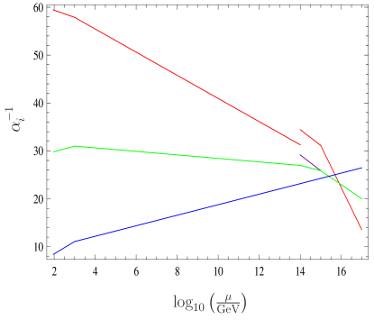
Figure 2: 1-loop running of the gauge couplings for the choice of scales $m_{SUSY}=1$ TeV, $v_{BL}=10^{14}$ GeV and $v_{R}=10^{15}$ GeV. The dependence of $\alpha_{i}^{-1}$, where $\alpha_{i}=\frac{g_{i}^{2}}{4\pi}$, on the energy scale $\mu$ is shown. Different gauge couplings are represented in the different energy regimes. For $\mu\in\left[m_{Z},v_{BL}\right]$ one has $\alpha_{3}^{-1}$ (blue), $\alpha_{L}^{-1}$ (green) and $\alpha_{Y}^{-1}$ (red). For $\mu\in\left[v_{BL},v_{R}\right]$ one has $\alpha_{3}^{-1}$ (blue), $\alpha_{L}^{-1}$ (green), $\alpha_{R}^{-1}$ (purple) and $\alpha_{BL}^{-1}$ (red). For $\mu>v_{R}$ one has $\alpha_{3}^{-1}$ (blue), $\alpha_{2}^{-1}\equiv\alpha_{L}^{-1}=\alpha_{R}^{-1}$ (green) and $\alpha_{BL}^{-1}$ (red).

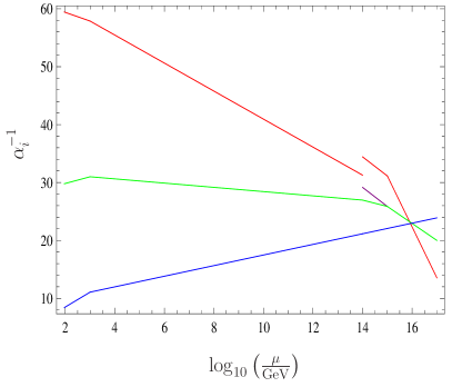
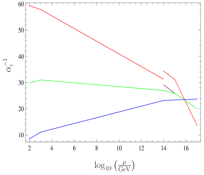
Figure 3: 1-loop running of the gauge couplings for the choice of scales $m_{SUSY}=1$ TeV, $v_{BL}=10^{14}$ GeV and $v_{R}=10^{15}$ GeV. Contrary to Figure 2, gauge coupling unification is obtained thanks to additional colored superfields. In the left panel, one triplet under $SU(3)_{c}$, singlet under the other gauge subgroups, is added at $m_{SUSY}$, whereas in the right panel five generations of the same superfield are added at $v_{BL}$. See Figure 2 for the color code.

Let us now discuss another important theoretical issue: $U(1)$ mixing. In the numerical implementation of the model we have chosen to break the left-right symmetric gauge sector down to the SM gauge group in one step in contrast to the heavy fields which we integrate out at two different scales. It would have been also possible to assume a gauge symmetry breaking in two steps, i.e. $SU(2)_{R}\times U(1)_{B-L}\rightarrow U(1)_{R}\times U(1)_{B-L}\rightarrow U(1)_{Y}$. However, the co-existence of two Abelian gauge groups introduces the possibility of kinetic mixing, because a term of the form $\kappa F_{\mu\nu}^{R}F^{B-L,\mu\nu}$ is allowed by gauge invariance Holdom:1985ag . Even if we assume that this term were absent at the $SU(2)_{R}$ breaking scale it would be introduced by RGE running already at 1-loop level because the two $U(1)$’s are not orthogonal for the given particle content. This might be indeed relevant because it has been shown that the effect of kinetic mixing can be sizable even if the scale where the $U(1)$’s coexist is rather short Malinsky:2005bi . Using the procedure presented in Fonseca:2011vn we have checked that the use of a two step breaking and running the parameters in the $U(1)_{R}\times U(1)_{B-L}$ basis is equivalent to the one step breaking and running the parameters under the resulting $U(1)_{Y}$. Here, we had to use 1-loop boundary conditions and threshold effects to compensate differences in the 2-loop running as we use 2-loop RGEs. Nevertheless, although kinetic mixing is conceptually interesting, in the model under consideration its effects on the phenomenology are minor.

III.2 Low energy spectrum

The introduction of additional superfields with masses below the GUT scale changes the RGEs not only for the gauge couplings but also for all MSSM soft terms. This in turn leads to changes in the electroweak scale supersymmetric mass spectra with respect to the standard CMSSM expectations. The CMSSM is defined by the following parameters: a common scalar mass $m_{0}$, a common gaugino mass parameter $M_{1/2}$ and common trilinear parameter $A_{0}$ which are specified at the GUT scale. In addition $\tan\beta$ is specified at the electroweak scale and the sign of $\mu$ is fixed. As discussed in section III.1 we do not have exact unification of the gauge couplings but expect that threshold corrections can account for the difference. Also the gaugino mass parameters are subject to corrections of the same size. Therefore we define the boundary conditions for the gaugino mass parameters at the GUT scale $m_{GUT}$ as follows:

$$M_{i}=\frac{\alpha_{i}}{\alpha_{BL}}M_{1/2}$$ (10)

For the calculation of the parameters at the SUSY scale we have used the complete 2-loop RGEs at all scales which have been derived with the Mathematica package SARAH Staub:2008uz ; Staub:2009bi ; Staub:2010jh . The numerical evaluation of the RGEs as well as the calculation of the loop corrected masses was done with SPheno Porod:2003um ; Porod:2011nf using the SPheno interface of SARAH Staub:2011dp . For more details about the numerical implementation see also Esteves:2010si .

An example spectrum is given in Figure 4 where we show two SUSY (and Higgs spectra) for a specific choice of CMSSM parameters ($m_{0}=600$ GeV, $M_{1/2}=700$ GeV, $A_{0}=0$, $\tan\beta=10$ and $\mu>0$). Dashed lines are the mass spectra for the pure CMSSM case, while the full lines have been calculated for the $\Omega$LR model with the specific choice of $v_{R}=v_{BL}=10^{14}$ GeV. These parameters were chosen to lie outside the region already excluded by the SUSY searches at the LHC experiments Khachatryan:2011tk ; Aad:2011hh ; daCosta:2011qk ; Chatrchyan:2011zy , but are otherwise arbitrary. These spectra should not be taken as predictions for the $\Omega$LR model, but serve only for the sake of discussing the main differences between this model and the pure CMSSM case.

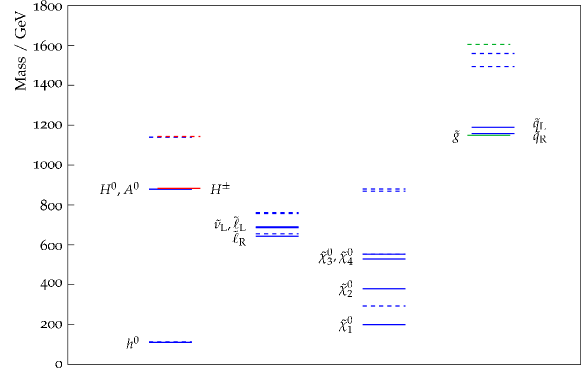
Figure 4: Example spectra comparing CMSSM with the $\Omega$LR model. Parameters have been chosen as $m_{0}=600$ GeV, $M_{1/2}=700$ GeV, $A_{0}=0$, $\tan\beta=10$, $\mu>0$ and $v_{R}=v_{BL}=10^{14}$ GeV. Full lines: $\Omega$LR, dashed line pure CMSSM. Note that in this example one has $m(\tilde{\chi}_{2}^{0})_{CMSSM}\simeq m(\tilde{\chi}_{4}^{0})_{\Omega LR}$ by accident.

In general, with $v_{BL}\leq v_{R}<m_{GUT}$, the $\Omega$LR has a lighter spectrum than CMSSM for the same parameters. One can understand this semi-quantitatively with the help of the following considerations.

Gaugino mass parameters run like gauge couplings do. Since in the $\Omega$LR model the running of the gauge couplings is changed with respect to the MSSM case, also gaugino masses are changed. Consider for example $M_{1}$. At 1-loop leading-log order we find

$$M_{1}(m_{SUSY}) = M_{1/2}\>\frac{\alpha_{Y}(m_{SUSY})}{\alpha_{BL}(m_{GUT})}$$

$$= M_{1/2}\>\left[X_{1}+X_{2}\left(-3l_{1}+l_{2}\right)\right]$$

where we have defined

$$X_{1} = \frac{5}{2}-\frac{3}{2}\frac{\alpha_{Y}(m_{SUSY})}{\alpha_{2}(m_{SUSY})}-\frac{15\alpha_{Y}(m_{SUSY})}{2\pi}\ln\left(\frac{m_{GUT}}{m_{SUSY}}\right)\,,\,X_{2}=\frac{3\alpha_{Y}(m_{SUSY})}{2\pi}$$ (12)

and

$$l_{1} = \ln\left(\frac{m_{GUT}}{v_{R}}\right)\,,\,l_{2}=\ln\left(\frac{v_{R}}{v_{BL}}\right).$$ (13)

Note that, due to their definition, $l_{1,2}\geq 0$, with $l_{1}=l_{2}=0$ in the CMSSM limit. One can easily check that $X_{1}>0$ and $X_{2}>0$. For $m_{GUT}=2\cdot 10^{16}$ GeV and $m_{SUSY}=1$ TeV one obtains roughly $X_{1}\simeq 0.424$ and $X_{2}\simeq 0.008$. Therefore, $M_{1}(m_{SUSY})$ decreases with $l_{1}$ and increases with $l_{2}$. In other words, one can decrease $M_{1}(m_{SUSY})$ with respect to the CMSSM value by using a large $l_{1}$ and $l_{2}=0$ and increase it only in the case $l_{2}>3l_{1}$. Similar equations hold for $M_{2}$ and $M_{3}$. However, at low energy ratios such as $M_{1}/M_{2}$ still follow the standard CMSSM expectations, only the relation to $M_{1/2}$ is changed.

Similarly, sfermion mass parameters can be written schematically as, $m_{\tilde{f}}^{2}\simeq m_{0}^{2}+c_{\tilde{f}}M_{1/2}^{2}$, where the coefficients $c_{\tilde{f}}$ are different for different sfermions and depend on $v_{R}$ and $v_{BL}$. Exact expressions are given in appendix A. One can show that for $v_{BL}\leq v_{R}<m_{GUT}$ the $c_{\tilde{f}}$ are always smaller than in the CMSSM limit, explaining why also the sfermions in the $\Omega$LR model are lighter than in CMSSM, see Figure 4. It is important to note, that gaugino masses change faster with $v_{R}$ than sfermion masses. We will come back to this point in the discussion about dark matter, see section IV.

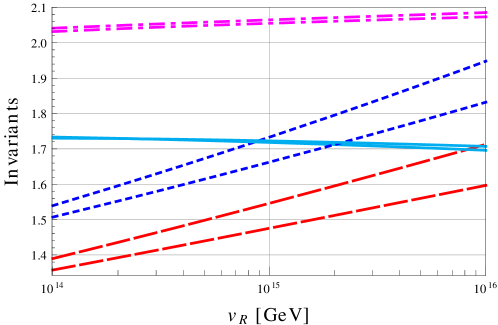
Figure 5: Invariant mass combinations QE/10 (purple, dashed-dotted lines), LE (red, dashed lines), QU (dark blue, dotted lines) and DL/10 (light blue, solid lines) as functions of $v_{R}$. $v_{BL}\in[10^{12},10^{14}]$ GeV, upper lines correspond to $v_{BL}=10^{12}$ GeV and lower lines to $v_{BL}=10^{14}$ GeV.

Individual SUSY masses depend strongly on the initial values of $m_{0}$ and $M_{1/2}$. However, one can form four different combinations (“invariants”) of soft SUSY breaking parameters, which we choose as

$$\begin{array}[]{c}LE\equiv(m_{L}^{2}-m_{e^{c}}^{2})/M_{1}^{2},\\ QE\equiv(m_{Q}^{2}-m_{e^{c}}^{2})/M_{1}^{2},\\ DL\equiv(m_{d^{c}}^{2}-m_{L}^{2})/M_{1}^{2},\\ QU\equiv(m_{Q}^{2}-m_{u^{c}}^{2})/M_{1}^{2},\end{array}$$ (18)

where at the leading-log level $m_{0}$ and $M_{1/2}$ drop out. Formulas for an analytical 1-loop leading-log calculation of these four invariants are given in appendix A.

Figure 5 shows the analytically calculated values of the invariants as a function of $v_{R}$ for two values of $v_{BL}$. The invariants depend more strongly on $v_{R}$ and only weakly on $v_{BL}$. As the figure shows, at leading order QE and DL show a very mild dependence on the scales $v_{R}$ and $v_{BL}$, while LE and QU decrease with decreasing $v_{R}$. At the $v_{R}$ scale one has $m_{L}^{2}=m_{e^{c}}^{2}$ and $m_{Q}^{2}=m_{u^{c}}^{2}=m_{d^{c}}^{2}$ due to parity conservation. This implies that the lower $v_{R}$ is, the smaller the difference between them at the SUSY scale is, which means that the $LE$ and $QU$ invariants can have values below the CMSSM prediction. We have checked that this effect is quite robust, and the theoretical uncertainties do not have much influence on it. In particular, these two invariants do not show any numerical dependence on $m_{GUT}$, due to cancellations among left and right contributions in the running from the GUT scale to $v_{R}$. This is an interesting result, since in CMSSM models with a type-II or type-III seesaw, all four invariants are always larger than their CMSSM limit for seesaw scales below the GUT scale Buckley:2006nv ; Hirsch:2008gh ; Esteves:2010ff . This allows, at least in principle, to distinguish between models with a high scale LR group and CMSSM models with type-II or type-III seesaw as the explanation for the observed neutrino masses.

Figure 5 shows the leading-log calculation. It is known in the case of seesaw based models, that there exist important 2-loop corrections and 1-loop threshold effects Hirsch:2008gh ; Esteves:2010ff . Similarly, also in the $\Omega$LR model important numerical corrections exist, as is shown in Figure 6. When the invariants are written including the effect of non-unification at the GUT scale, see appendix A, they reproduce qualitatively the numerical results. However, as shown in Figure 6 quantitatively important shifts are obtained going from leading-log to (numerically solved) full 1-loop calculation. Even going from 1-loop to 2-loop calculation, numerically important differences are found.

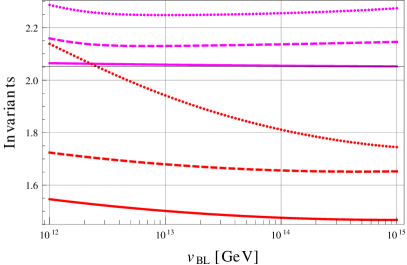
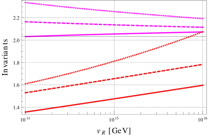
Figure 6: Invariant mass combinations QE/10 and LE as functions of $v_{BL}$ (left) and $v_{R}$ (right). The color code is the same as in Figure 5. Solid lines correspond to the analytical approximation, dashed lines to 1-loop numerical results and dotted lines to 2-loop numerical results. Similar deviations are found for the other two invariant mass combinations.

To summarize, the invariants are good model discriminators in principle. Especially noteworthy, in the $\Omega$LR model LE and QU are expected to be below their CMSSM limit. However, to identify such spectrum distortions, once the SUSY mass spectrum is measured, will require highly accurate measurements and therefore measurements at an ILC.

III.3 Lepton flavour violation and the role of $\theta_{1,2}$

Flavour violation in leptonic processes has attracted a lot of attention in the experimental community. Decays like $\mu\to e\gamma$ have been searched for decades, without any positive result. Very recently, the MEG experiment meg has published the results of the analysis of the data collected in 2009 and 2010 Adam:2011ch , setting the new bound $\text{Br}(\mu\to e\gamma)<2.4\cdot 10^{-12}$. This impressive experimental limit strongly constrains models with extended lepton sectors, such as the $\Omega$LR model.

The branching ratio for $l_{i}\to l_{j}\gamma$ can be written as Kuno:1999jp

$$\text{Br}(l_{i}\to l_{j}\gamma)=\frac{48\pi^{3}\alpha}{G_{F}^{2}}\left(|A_{L}^{ij}|^{2}+|A_{R}^{ij}|^{2}\right)\text{Br}(l_{i}\to l_{j}\nu_{i}\bar{\nu}_{j})\thickspace.$$ (19)

The couplings $A_{L}$ and $A_{R}$ are generated at the 1-loop level. The relation between these couplings and the slepton soft masses is given approximately by

$$A_{L}^{ij}\sim\frac{(m_{L}^{2})_{ij}}{m_{SUSY}^{4}}\quad,\quad A_{R}^{ij}\sim\frac{(m_{e^{c}}^{2})_{ij}}{m_{SUSY}^{4}}\thickspace,$$ (20)

where $m_{SUSY}$ is a typical supersymmetric mass. In the derivation of this estimate it has been assumed that (a) chargino/neutralino masses are similar to slepton masses and (b) A-terms mixing left-right transitions are negligible.

Note that, due to the negligible off-diagonal entries in $m_{e^{c}}^{2}$, a pure seesaw model predicts $A_{R}\simeq 0$. On the contrary, in reference Esteves:2010si it was pointed out that a left-right symmetry at high energies induces non-negligible off-diagonal elements in $m_{e^{c}}^{2}$, giving additional contributions to LFV processes. In fact, taking into account the running from the GUT scale to the $v_{R}$ scale, the off-diagonal elements of the slepton soft masses at 1-loop order can be written in leading-log approximation as Chao:2007ye ; Esteves:2010si

$$\left(m_{L}^{2}\right)_{ij}|_{v_{R}} = -\frac{1}{4\pi^{2}}\left(3ff^{\dagger}+\sum_{k=1}^{2}Y_{L}^{(k)}Y_{L}^{(k)\>\dagger}\right)_{ij}(3m_{0}^{2}+A_{0}^{2})\ln\left(\frac{m_{GUT}}{v_{R}}\right)\thickspace,$$ (21)

$$\left(m_{e^{c}}^{2}\right)_{ij}|_{v_{R}}=\left(m_{L^{c}}^{2}\right)_{ij}|_{v_{R}} = -\frac{1}{4\pi^{2}}\left(3f^{\dagger}f+\sum_{k=1}^{2}Y_{L}^{(k)\>\dagger}Y_{L}^{(k)}\right)_{ij}(3m_{0}^{2}+A_{0}^{2})\ln\left(\frac{m_{GUT}}{v_{R}}\right)\thickspace,$$ (22)

which are of the same size in the CP conserving case. The $A$ parameters also develop LFV off-diagonals in the running. We do not give the corresponding approximated equations because they do not lead to qualitatively new features.

The angular distribution of the outgoing positron at, for example, the MEG experiment could be used to discriminate between left- and right-handed polarized states Okada:1999zk ; Hisano:2009ae . If MEG is able to measure the positron polarization asymmetry, defined as

$$A_{LR}=\frac{|A_{L}|^{2}-|A_{R}|^{2}}{|A_{L}|^{2}+|A_{R}|^{2}},$$ (23)

we will have an additional tool to distinguish from pure seesaw models, where $A_{LR}\simeq 1$ is predicted.

We extend here the discussion of ref. Esteves:2010si , addressing the influence of the high energy parameters on low energy observables. As explained in section II, the mixing angles of the bidoublets at the $v_{R}$ scale have a very strong impact on low energy LFV processes. As is shown in eqs. (6) and (7), this is due to their relation to the Yukawa parameters. If the bidoublet couplings are tuned such that $\theta_{1}$ and $\theta_{2}$ get very close values, the entries of the Yukawa matrix $Y_{L}$ will become very large, which in turn will lead to large running effects for the soft squared masses of the sleptons. Therefore, we expect a strong correlation between $s_{21}=\sin(\theta_{2}-\theta_{1})$ and the size of the LFV processes.

The left side of Figure 7 shows such correlation for a particular but representative set of parameters. We note that a proper choice of $\theta_{2}-\theta_{1}$ can enhance (or suppress) the $l_{i}\to l_{j}\gamma$ branching ratios by several orders of magnitude. Moreover, special values for $\theta_{2}-\theta_{1}$ are found where the $\tau$ decays have strong cancellations. Their origin can be traced back to the flavour structure of the LFV entries in $m_{L}^{2}$ and $m_{e^{c}}^{2}$.

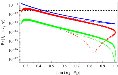
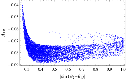
Figure 7: To the left, $\text{Br}(\mu\to e\gamma)$ (blue), $\text{Br}(\tau\to\mu\gamma)$ (red) and $\text{Br}(\tau\to e\gamma)$ (green) as a function of $|\sin(\theta_{2}-\theta_{1})|$. The horizontal line shows the current MEG bound $\text{Br}(\mu\to e\gamma)<2.4\cdot 10^{-12}$. To the right, the positron polarization asymmetry $A_{LR}$ as a function of $|\sin(\theta_{2}-\theta_{1})|$. Both figures have been made fitting neutrino data with the flavour structure in $Y_{\nu}$ and taking the parameter choice $M_{S}=10^{12}$ GeV, $v_{BL}=v_{R}=10^{15}$ GeV for the CMSSM point $m_{0}=120$ GeV, $M_{1/2}=600$ GeV, $\tan\beta=10$, $A_{0}=0$ and $\mu>0$.

The RGE running from $m_{GUT}$ to $v_{R}$ introduces LFV entries in $m_{L}^{2}$ and $m_{e^{c}}^{2}$ proportional to $\sum_{k}Y_{L}^{(k)}Y_{L}^{(k)\>\dagger}$ (the dagger is to be exchanged for the case of $m_{e^{c}}^{2}$, which makes no difference if CP is conserved). Expanding this expression in terms of $Y_{e}$ and $Y_{\nu}$, the Yukawa couplings at $v_{R}$, one obtains

$$\sum_{k}Y_{L}^{(k)}Y_{L}^{(k)\>\dagger}=\frac{1}{s^{2}_{21}}\left[Y_{\nu}Y_{\nu}^{\dagger}+Y_{e}Y_{e}^{\dagger}+c_{21}(Y_{e}Y_{\nu}^{\dagger}+Y_{\nu}Y_{e}^{\dagger})\right]$$ (24)

where $c_{21}=\cos(\theta_{2}-\theta_{1})$. For the observable $\text{Br}(l_{i}\to l_{j}\gamma)$ we have to compute $(\sum_{k}Y_{L}^{(k)}Y_{L}^{(k)\>\dagger})_{ij}$, with $i\neq j$. The $Y_{e}Y_{e}$ piece can be neglected, since $Y_{e}$ is almost diagonal (we choose to work in the basis in which $Y_{e}$ is diagonal at the electroweak scale). Furthermore, in the approximation $m_{l_{i}}\gg m_{l_{j}}$ one can also neglect the $Y_{\nu}Y_{e}^{\dagger}$ piece, since it will be proportional to $m_{l_{j}}$. Therefore, using eqs. (19) and (20), one finds

$$\text{Br}(l_{i}\to l_{j}\gamma)\propto\frac{1}{s^{4}_{21}}|(Y_{\nu}Y_{\nu}^{\dagger}+c_{21}Y_{e}Y_{\nu}^{\dagger})_{ij}|^{2}$$ (25)

From eq. (25) one can see that as $\theta_{1}$ and $\theta_{2}$ get closer $s_{21}\to 0$ and one gets an enhancement. The interesting new point is the interplay of the two terms as for specific values of $\theta_{2}-\theta_{1}$ cancellations occur. In case of of $\text{Br}(\mu\to e\gamma)$ this hardly occurs as in general the $\mu$-Yukawa coupling is much smaller than the $|(Y_{\nu})_{ij}|$ and a cancellation is not possible. On the contrary, the $\tau$-Yukawa coupling is comparable to $Y_{\nu}$ in large parts of interesting parameter space, allowing for potential cancellations.

However, we want to stress that the position and the degree of these cancellations depend on the high energy VEVs $v_{BL}$ and $v_{R}$ and thus one cannot determine $\theta_{2}-\theta_{1}$ uniquely. Moreover, this connection between leptons and bidoublet mixing angles is lost if one fits neutrino data using the superpotential coupling $f$, which gives rise to the Majorana mass of the right-handed neutrino. In this possibility, called ’$f$ fit’ in Esteves:2010si , there is no dependence on the bidoublet mixing angles, since $f$ couples the leptons to the $\Delta$ triplets, but not to the bidoublets. For completeness we note that also the positron polarization asymmetry $A_{LR}$ depends somewhat on $\theta_{2}-\theta_{1}$ as can be seen on the right side of Figure 7.

Finally, we have checked that this strong dependence on $\theta_{1,2}$ is not present in the quark sector. Flavour violating processes, such as $b\to s\gamma$, are very weakly affected by the bidoublet mixing angles and the phenomenology follows very closely the well-known results of the CMSSM. This is due to the fact that flavour violation in the (s)quark sector is dominated by the CKM matrix. In other words, the $\Omega$LR model is a minimal flavour violating one Buras:2000dm ; DAmbrosio:2002ex .

IV Dark matter

Astrophysical observations and the data from WMAP Komatsu:2010fb put on solid grounds the existence of non-baryonic dark matter in the universe. The PDG Nakamura:2010zzi quotes the value $\Omega_{\rm DM}h^{2}=0.110\pm 0.006$ at $1\sigma$ C.L. It is well-known that with this low value of $\Omega_{\rm DM}h^{2}$ only a few, very specific regions in the parameter space of CMSSM can give the correct relic density for the neutralino Griest:1990kh . These are known as (in no specific order) (i) the stau co-annihilation region Ellis:1998kh ; (ii) the stop co-annihilation region Boehm:1999bj ; Ellis:2001nx ; Edsjo:2003us ; (iii) the focus point line Feng:1999zg ; Feng:2000gh and (iv) the Higgs funnel Griest:1990kh .

In any of the co-annihilation regions the relic density of the lightest neutralino, which in the above cases (i) and (ii) is mostly bino, is reduced with respect to naive expectations by a close mass degeneracy between the neutralino and the NLSP. Any changes in the SUSY spectra can then have a rather large impact on the calculated $\Omega_{\tilde{\chi}^{0}_{1}}h^{2}$. In the focus point region a comparatively small value of $\mu$, with respect to the rest of the CMSSM parameter space, leads to an increased higgsino content in the lightest neutralino. This in turn leads to a larger coupling of the LSP to the $Z^{0}$, thus reducing the relic density. The fourth allowed region, the Higgs funnel, appears for high values of $\tan\beta$ and for parameters where the CP-odd Higgs scalar $A$ has a mass which is twice the LSP mass. In this case there is an s-channel resonant enhancement of the neutralino annihilation cross section and large values of $\tan\beta$ are needed for this resonance to be effective, since the width of $A$ is large at large $\tan\beta$. All of the regions discussed above have been extensively studied in the CMSSM Ellis:1983ew ; Griest:1990kh ; Drees:1992am ; Jungman:1995df and in some extensions of it, like CMSSM plus seesaw of either type-II or type-III Esteves:2009qr ; Esteves:2010ff .

Below we discuss the changes for these allowed regions for the $\Omega$LR model. We have used SPheno to compute the low energy spectrum and used it as an input for micrOmegas Belanger:2006is to obtain the value for $\Omega_{\tilde{\chi}^{0}_{1}}h^{2}$. To include effects of flavour violation, we have created suitable model files for micrOmegas with SARAH. In the present setup the main effect on dark matter is via changes in spectrum (see section III.2). For low $v_{BL}$ or $v_{R}$ the dark matter allowed regions are reduced compared to the CMSSM. We have found this effect for the stau co-annihilation, stop co-annihilation, Higgs funnel and focus point regions and discuss these regions in turn.

IV.1 Non-flavoured dark matter allowed regions in $\Omega$LR

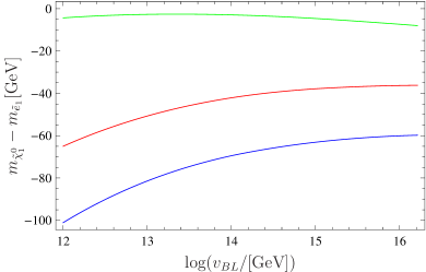
Figure 8: Stau co-annihilation. On the left: mass difference between the lightest neutralino and the lightest stau vs. $v_{BL}$ for three different values of $v_{R}=10^{12}$ (blue), $10^{14}$ (red) and $10^{16}$ GeV (green). On the right: resulting dark matter relic density $\Omega h^{2}$. The gray band shows the $\Omega h^{2}=[0.1018,0.1228]$. The other input parameters have been chosen as: $m_{0}=105$ GeV, $M_{1/2}=600$ GeV, $\tan\beta=10$, $A_{0}=0$ GeV.

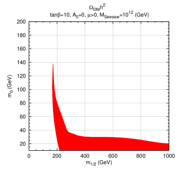
Figure 9: Dark Matter allowed regions for $\tan\beta=10$, and $v_{BL}=v_{R}=1.5\times 10^{15}$ GeV (left) and $v_{BL}=v_{R}=10^{16}$ GeV (right). For this figure we have chosen a low seesaw scale, $M_{S}=10^{12}$ GeV, which assures that the LFV constraints are respected.

IV.1.1 Stau co-annihilation

As discussed in section III.2, lowering the values of $v_{BL}$ and $v_{R}$ leads in general to a lighter spectrum compared to the pure CMSSM case, for the same values of CMSSM parameters. In Figure 8 we show an example for the mass difference between the lightest neutralino and the lightest scalar tau for three values of $v_{R}$ as a function of $v_{BL}$. Since the mass of the bino decreases faster than the mass of the stau, the mass difference increases and this in turn leads to a larger value of the neutralino density, as shown in the plot on the right, because co-annihilation becomes ineffective for $\Delta_{m}=m_{\tilde{\tau}_{1}}-m_{\chi^{0}_{1}}$ larger than a few GeV. Note that the CMSSM parameters in this example have been chosen to give approximately the correct relic density for $v_{R}\simeq 10^{16}$ GeV.

Two examples of allowed stau co-annihilation regions are then shown in Figure 9. The figure shows the 3 $\sigma$ allowed regions for $\tan\beta=10$, and $v_{BL}=v_{R}=1.5\times 10^{15}$ GeV (left) and $v_{BL}=v_{R}=10^{16}$ GeV (right). Lowering $v_{R}$ (and $v_{BL}$) shifts the allowed region towards smaller values of $m_{0}$. Depending on the values of $\tan\beta$ and $A_{0}$ chosen, for values of roughly $v_{BL}=v_{R}\sim 10^{15}$ GeV the stau coannihilation line disappears completely. The observation of a SUSY particle spectrum consistent with the stau co-annihilation region could thus be turned into a lower limit on $v_{BL}$ and $v_{R}$ within CMSSM, at least in principle.

However, as has been noted in section III.2, the effect of $v_{R}$ on $M_{1}$ is stronger and inverse to the one of $v_{BL}$. We have checked that it is possible to obtain a stau-coannihilation region slightly above the CMSSM expected region (for any fixed $\tan\beta$ and $A_{0}$) for values of $v_{R}$ close to the GUT scale and $v_{BL}$ low. Thus, the stau coannihilation can give a lower limit on $v_{R}$ only as a function of the (assumed) value of $v_{BL}$.

IV.1.2 Stop co-annihilation

With typical choices of CMSSM parameters the squarks are much heavier then the LSP. However, if the off-diagonal elements in the squark mass matrices are significant, the lighter mass eigenstates have their masses lowered and the lighter stop can be almost degenerate in mass with the lightest neutralino. This stop co-annihilation has been studied in the literature Boehm:1999bj ; Ellis:2001nx ; Edsjo:2003us and happens for instance if the soft breaking parameter $A_{0}$ has a large value We also explored this possibility in the present setup. Figure 10 shows an example. In this plot, the CMSSM parameters where chosen to be $m_{0}=630$ GeV, $M_{1/2}=400$ GeV, $\tan\beta=10$, $A_{0}=-2$ TeV and $\mu>0$, which leads to a mass difference between stop and neutralino below 2 GeV in the pure CMSSM limit. Lowering $v_{R}$ or $v_{BL}$ below the GUT scale, this mass difference again increases, rendering co-annihilation ineffective. The lowest possible values for $v_{BL}$ and $v_{R}$ in this scenario are usually found in the region $v_{BL}\sim v_{R}$, as the figure shows. We found no combination of parameters which improves the result shown in the figure by more than a few GeV. Our conclusion is therefore, that the stop co-annihilation region vanishes for low intermediate scales, similarly to the stau-coannihilation region. Observation of a SUSY spectrum consistent with stop co-annihilation could therefore be interpreted as a lower limit on $v_{R}$ and $v_{BL}$.

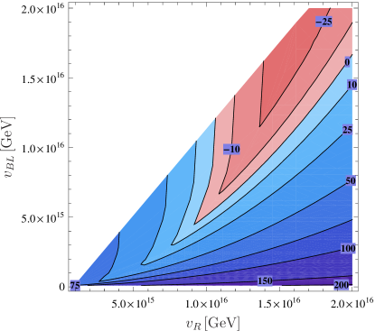
Figure 10: $m_{\tilde{\chi}_{1}^{0}}-m_{\tilde{t}_{1}}$ contours in the $v_{BL}-v_{R}$ plane. The CMSSM parameters take the following values: $m_{0}=630$ GeV, $M_{1/2}=400$ GeV, $\tan\beta=10$, $A_{0}=-2$ TeV and $\mu>0$.

IV.1.3 Higgs funnel

Figure 11: The allowed region for $\Omega_{\tilde{\chi}^{0}_{1}}h^{2}$ in the $m_{0}$-$M_{1/2}$ plane for $\tan\beta=53$, $v_{BL}=v_{R}=10^{16}$ GeV. For this figure we have chosen a low seesaw scale, $M_{S}=10^{11}$ GeV, which assures that the LFV constraints are respected.

As in the previous two examples, we have found that also the Higgs funnel region depends rather strongly on the choice of $v_{R}$ and $v_{BL}$. As mentioned above, at large values of $\tan\beta$, typically $\tan\beta\geq 50$ the width of the CP-odd Higgs boson A can be large enough so that there is a s-channel resonance for the neutralino pair annihilation in the region $2m_{\chi^{0}_{1}}\simeq m_{A}$. An example for this Higgs funnel region is shown in Figure 11.

In the $\Omega$LR model the Higgs funnel region disappears when the intermediate scales are lowered below a certain limit. This is due to the existence of an upper limit on $\tan\beta$, stronger in the $\Omega$LR model than in CMSSM, caused by the requirement of (1) perturbativity of the bottom and tau Yukawa couplings, and (2) stability of the electroweak symmetry breaking minimum of the Higgs potential. In the CMSSM this limit is roughly $\tan\beta\simeq 55-60$. In the $\Omega$LR model this limit depends on $v_{R}$, and becomes stronger when this high energy scale is lowered. This can be understood, in principle, from the fact that the lower $v_{R}$ is, the larger the RGE effects on the Yukawa couplings are. As shown in Figure 12, which should be taken as an illustrative example, for a given value of $v_{R}$ one can always find an upper limit on $\tan\beta$, which in the limit $v_{R}$ approaching $m_{GUT}=2\cdot 10^{16}$ GeV recovers the usual CMSSM limit on $\tan\beta$. For lower values of $v_{R}$, therefore, there is an upper limit on the A width. The allowed Higgs funnel region becomes smaller until for a certain value of $v_{R}$ it disappears completely. We have also observed additional minor effects that can play a role in the determination of the correct relic density. For example, a dependence of the higgsino component of the LSP on $v_{BL}$ has been found. Again, this can lead to the disappearance of the Higgs funnel. Therefore, if SUSY is discovered with large $\tan\beta$, this could again be interpreted as a lower limit on $v_{R}$.

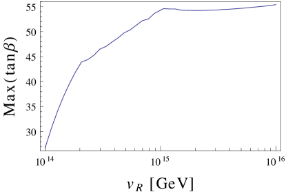
Figure 12: Upper limit on $\tan\beta$ as a function of $v_{R}$ for $v_{BL}=10^{14}$ GeV. The figure was obtained for the choice of CMSSM parameters $m_{0}=M_{1/2}=1.5$ TeV, $A_{0}=0$ and $\mu>0$.

IV.1.4 Focus point

The focus point is also affected by the running of the parameters above the parity breaking scale. The observed dark matter relic density is obtained in this region thanks to annihilation into $Z^{0}$ bosons, a process which is only effective when the higgsino component of the lightest neutralino is sufficiently large. This is provided by a small $\mu$ parameter, $\mu\sim M_{1}$.

As explained, $M_{1}(m_{SUSY})$ is typically smaller in the $\Omega$LR model than in the CMSSM. When one lowers the high energy VEVs $v_{BL}$ and/or $v_{R}$, the resulting $M_{1}(m_{SUSY})$ gets lowered as well, see eq. (III.2). Therefore, the required tuning with the $\mu$ parameter can only be obtained by increasing $M_{1/2}$. A shift of the focus point region towards larger values of $M_{1/2}$ is thus expected.

This expectation has been check numerically. Figure 13 shows $\Omega_{DM}h^{2}$ as a function of $M_{1/2}$ for the choice of parameters $m_{0}=2.5$ TeV, $\tan\beta=30$, $A_{0}=0$ and $\mu>0$. As $v_{BL}$ and $v_{R}$ are decreased, one needs to go to larger values of $M_{1/2}$ in order to reproduce the observed relic abundance. We find that for $v_{BL}=v_{R}\sim 10^{15}$ GeV one cannot make the annihilations sufficiently effective and the focus point disappears (for this particular choice of parameters). Note that in this figure all curves reach their minimum, lower $M_{1/2}$ values would spoil electroweak symmetry breaking. We also would like to emphasize that the dependence on $v_{BL}$ and $v_{R}$ is very strong. This can be clearly seen from the non-negligible shift in $M_{1/2}$ obtained when one goes from $v_{BL}=v_{R}=m_{GUT}=2\cdot 10^{16}$ GeV to just $v_{BL}=v_{R}=1.9\cdot 10^{16}$ GeV.

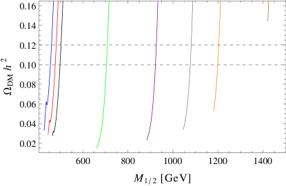
Figure 13: $\Omega_{DM}h^{2}$ as a function of $M_{1/2}$ for the choice of parameters $m_{0}=2.5$ TeV, $\tan\beta=30$, $A_{0}=0$ and $\mu>0$. From left to right the different curves correspond to $v_{BL}=v_{R}=[2\cdot 10^{16}$, $1.9\cdot 10^{16}$, $1.8\cdot 10^{16}$, $10^{16}$, $5\cdot 10^{15}$, $3\cdot 10^{15}$, $2\cdot 10^{15}$, $10^{15}]$ GeV. All curves reach their minimum, lower $M_{1/2}$ values would spoil electroweak symmetry breaking. The dashed horizontal lines show the values $\Omega_{DM}h^{2}=[0.1018,0.1228]$.

We also found a clear dependence of $\Omega_{DM}h^{2}$ on the angles $\theta_{1,2}$, as shown in figure 14. This can be easily understood from the matching conditions at the $SU(2)_{R}$ breaking scale, eqs. (6) and (7). The running of the soft parameter $m_{H_{u}}^{2}$ is strongly affected by the quark Yukawas $Y_{Q}^{1,2}$ at energies above $v_{R}$. This leads to different values for the $\mu$ parameter at the SUSY scale, affects the annihilation cross-section of the lightest neutralino and modifies its relic abundance. Another relevant parameter is $m_{top}$, which also has a strong impact on $m_{H_{u}}^{2}$. In our runs we have used the value $m_{top}=171.1$ GeV. However, we point out that the effect of taking a different value for $m_{top}$ can be compensated by choosing proper values for the angles $\theta_{1,2}$.

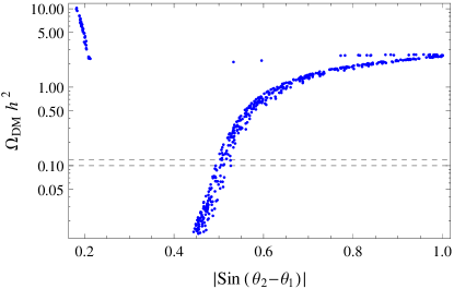
Figure 14: $\Omega_{DM}h^{2}$ as a function of $\sin(\theta_{2}-\theta_{1})$ for the choice of parameters $m_{0}=2.5$ TeV, $M_{1/2}=708$ GeV, $\tan\beta=30$, $A_{0}=0$, $\mu>0$ and $v_{BL}=v_{R}=10^{16}$ GeV. The dashed horizontal lines show the values $\Omega_{DM}h^{2}=[0.1018,0.1228]$.

IV.2 Flavoured co-annihilation

The $\Omega$LR model is in principle well suited for flavoured co-annihilation Choudhury:2011um . The $\tilde{\tau}_{R}$ can be made lighter by flavour contributions, making it possible to have co-annihilation with the lightest neutralino in points of parameter space where it would be impossible without flavour effects. Moreover, to obtain the correct relic density one must include flavour violating processes, like $\tilde{\tau}_{R}\tilde{\chi}_{1}^{0}\to\gamma\mu$ or $\tilde{\tau}_{R}\tilde{\tau}_{R}\to\tau\mu$.

It is possible to find regions in the $m_{0}$-$M_{1/2}$ plane where $\text{Br}(\mu\to e\gamma)$ and the other LFV decays respect the experimental limits while having flavoured co-annihilation. In addition to the usual fine-tuning that is required in the CMSSM to obtain the observed dark matter relic density, flavoured co-annihilation also requires to tune the neutrino mixing parameters in order to suppress $\text{Br}(\mu\to e\gamma)$. In order to have large flavour effects in the slepton sector, to be able to reduce the mass of the $\tilde{\tau}_{R}$ and, at the same time, respect the experimental limits, one must find values for $\theta_{13}$ (the reactor angle) and $\delta$ (the Dirac phase) that allow cancellations in $\text{Br}(\mu\to e\gamma)$. We find that this cancellation is more effective if the mass of the lightest neutrino is non-zero. The $\tau$ LFV decays are put under control by choosing $m_{0}$ and $M_{1/2}$ sufficiently large. Figure 15 shows one example. On the left panel the cancellation of $\text{Br}(\mu\to e\gamma)$ is obtained with $\delta=\pi$ and $\theta_{13}=8^{\circ}$, while on the right panel with $\theta_{13}=9.5^{\circ}$. Note that this occurs for different values of $m_{0}$ and $M_{1/2}$.

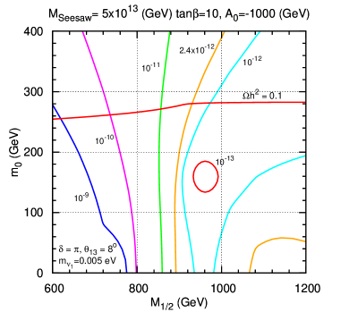
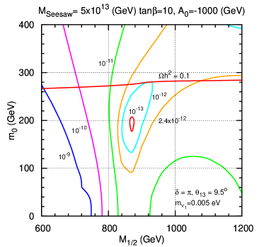
Figure 15: $\Omega_{\tilde{\chi}^{0}_{1}}h^{2}$ and $\text{Br}(\mu\to e\gamma)$ contour plots in the $m_{0}$-$M_{1/2}$ plane for $\delta=\pi$, $\theta_{13}=8^{0}$ (left) and $\theta_{13}=9.5^{0}$ (right). The other parameters are indicated in the figures, except for the $\Omega$LR parameters, $v_{R}=10^{15}$ GeV and $v_{BL}=10^{14}$ GeV.

Let us comment on some particularities of the $\Omega$LR model concerning cancellations in $\text{Br}(\mu\to e\gamma)$. It turns out that, contrary to the minimal type-I seesaw model, where the cancellation in $\text{Br}(\mu\to e\gamma)$ occurs for a Dirac phase $\delta=\pi$ and for $\theta_{13}\simeq 5^{\circ}$, independently of the $m_{0}$ and $M_{1/2}$ values, for the $\Omega$LR model the cancellation occurs for different values of $\theta_{13}$ depending on $m_{0}$ and $M_{1/2}$. This fact might be puzzling, since the Yukawa structure that appears in the running of $m_{L}^{2}$ and $m_{e}^{2}$ is the same as in the type-I seesaw. Therefore, if one wants to cancel this combination of Yukawas by choosing the right $\theta_{13}$, it should be possible to use the same value in type-I and $\Omega$LR, and this is not the case.

The key point is that, in addition to $m_{L}^{2}$ and $m_{e}^{2}$, one also has a soft trilinear term contribution, $T_{e}$, to $\text{Br}(\mu\to e\gamma)$. This contribution is present in both amplitude coefficients, $A_{L}$ and $A_{R}$, and suppressed in the type-I seesaw due to its proportionality to charged lepton masses. However, in the $\Omega$LR model this contributions turns out to be much larger. This can be understood from the RGEs. The 1-loop RGEs for $T_{e}$ in the parity conserving regime Staub:Web contain terms of the type $f^{\dagger}fY_{L}^{(k)}$ with $k=1,2$. This will lead to two pieces after applying the matching conditions at $v_{R}$, see eq. (7): the conventional $f^{\dagger}fY_{e}$, which is charged lepton mass suppressed, and the new $f^{\dagger}fY_{\nu}$, which is not suppressed and gives rise to new contributions to $\text{Br}(\mu\to e\gamma)$.

This conclusion has been checked numerically, by studying the dependence of the different contributions to $\text{Br}(\mu\to e\gamma)$ on $\theta_{13}$. We found that for large $A_{0}$ the $T_{e}$ contribution is dominant, which explains why $\text{Br}(\mu\to e\gamma)$ does not cancel for $\theta_{13}\simeq 5^{\circ}$ as in the minimal type-I seesaw. For $A_{0}=0$ the $T_{e}$ contribution is much smaller, and thus one finds an approximate cancellation for $\theta_{13}\simeq 5^{\circ}$, as expected.

V LHC phenomenology

In this section we investigate predictions for the LHC phenomenology of the $\Omega$LR model. The effects of the heavy states are two-fold: they change the spectrum and induce flavour violating off-diagonal elements in the slepton and sneutrino mass matrices. The changes of the spectrum can lead to a potentially measurable difference between the states which are mainly selectron- and smuon-like Allanach:2008ib ; Buras:2009sg ; Abada:2010kj ; Esteves:2010si . Here we are going to focus on the lepton flavour violation within the SUSY cascade decays as they occur for example in the decay chain

$$\tilde{q}_{L}\to q\tilde{\chi}^{0}_{2}\to qe^{-}{\tilde{l}}_{i}^{+}\to qe^{-}\mu^{+}\tilde{\chi}^{0}_{1}$$ (26)

As already stated above, in this model one has additional lepton flavour mixing for the R-sleptons as opposed to the usual seesaw mechanisms where the lepton flavour mixing is in the left sector only.

In Figure 16 we show total rates for $pp\to\tilde{\chi}^{0}_{2}\to ll^{\prime}\tilde{\chi}^{0}_{1}$ with $l\neq l^{\prime}$ as a function of $M_{1/2}$ for $\sqrt{s}=14$ TeV, $m_{0}=100$ GeV, $A_{0}=0$, $\tan\beta=10$ and $\mu>0$ for different values of $v_{BL}=v_{R}$. Choosing $v_{BL}=v_{R}$ implies that one has approximately the same amount of flavour mixing for left- and right-sleptons. Here we have summed over all initial states containing squarks and gluinos and over all cascade decays leading to a $\tilde{\chi}^{0}_{2}$. We have furthermore required that exactly one $\tilde{\chi}^{0}_{2}$ decays lepton flavour violating and that no additional lepton occurs in any of the cascade decays of the corresponding event. For the calculation of the cross section we have used the FASER-LHC package BenFaser which is based on the program PROSPINO Beenakker:1996ed . Recent ATLAS daCosta:2011qk and CMS Chatrchyan:2011zy data constrain already gluino and squark masses and are mainly interpreted in the context of the CMSSM. In our model the spectrum differs with respect to the CMSSM but we expect that for our choice of parameters gluino masses are excluded below about 1 TeV. For this reason we put dashed lines if the gluino mass is below this bound and full lines if the value is above.

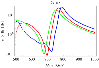
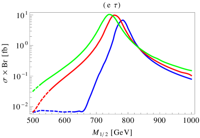
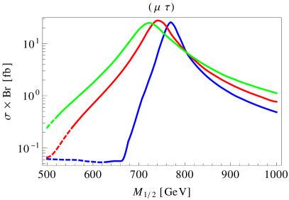
Figure 16: $\sigma\times\text{Br}$ for $pp\to\tilde{\chi}_{2}^{0}\>X\to\tilde{\chi}_{1}^{0}\>e\>\mu\>X$ (upper left plot), $pp\to\tilde{\chi}_{2}^{0}\>X\to\tilde{\chi}_{1}^{0}\>e\>\tau\>X$ (upper right plot), $pp\to\tilde{\chi}_{2}^{0}\>X\to\tilde{\chi}_{1}^{0}\>\mu\>\tau\>X$ (lower plot), as a function of $M_{1/2}$ for $\sqrt{s}=14$ TeV. The curves correspond to different values for $v_{BL}=v_{R}$: $10^{14}$ GeV (blue), $5\times 10^{14}$ GeV (red) and $10^{15}$ GeV (green). The other CMSSM parameters have been fixed to: $m_{0}=100$ GeV, $A_{0}=0$ GeV, $\tan\beta=10$ and $\mu>0$. The seesaw scale $M_{S}$ has been adjusted at each point in order to get $\text{Br}(\mu\to e\gamma)$ close to but smaller than $2.4\cdot 10^{-12}$. Regions with a gluino mass below $1$ TeV are denoted with dashed lines.

The neutrino Yukawa couplings are chosen such that Br$(\mu\to e\gamma)$ is close to its current bound of $2.4\cdot 10^{-12}$. Here we assumed that the right-handed neutrinos are degenerate in mass. Let us first discuss the final states containing a $\tau$-lepton. We see an increase of the rates with increasing $M_{1/2}$ until it reaches a maximum between 700 and 800 GeV depending on the value $v_{BL}=v_{R}$ and then drops with increasing $M_{1/2}$. This behaviour is due to an interplay of three effects: (i) with increasing $M_{1/2}$ larger values for the entries of $Y_{\nu}$ are allowed as Br($\mu\to e\gamma$) gets suppressed by the heavier spectrum. This implies larger flavour violating decay rates of $\tilde{\chi}^{0}_{2}$. (ii) For fixed $m_{0}$ the left sleptons are heavier than $\tilde{\chi}^{0}_{2}$ for small $M_{1/2}$ and they have about the same mass for $M_{1/2}$ in our examples between 500 and 600 GeV depending on the value of $v_{BL}=v_{R}$. (iii) Heavier squark and gluino masses imply reduced cross sections. The shift of the maxima to higher values of $M_{1/2}$ with decreasing $v_{BL}=v_{R}$ is again a consequence of the modified spectrum: smaller values of $v_{BL}=v_{R}$ imply smaller gaugino masses and increased ratios of slepton masses over gaugino masses at the electroweak scale for fixed $M_{1/2}$, which shifts the $M_{1/2}$ value where neutralino decays into on-shell L-sleptons are kinematically allowed. For completeness we note that the total rates can go up to 10 (30) fb in case of the $e\tau$ ($\mu\tau$) implying at most a few thousands events if the design luminosity of 100 fb^-1 per year can be achieved. The reduced values for the $e\tau$ channel compared to the $\mu\tau$ is a consequence of neutrino physics as we require tri-bimaximal mixing. This leads to $m^{2}_{L,13}$/$m^{2}_{L,23}\simeq m^{2}_{e^{c},13}$/$m^{2}_{e^{c},23}\sim m_{sol}/m_{atm}$ where $m_{sol}$ and $m_{atm}$ are the solar and atmospheric neutrino mass scale, respectively.

In case of the $e$-$\mu$ final state in Figure 16 we see a second maximum at lower values of $M_{1/2}$ in a region where the final states containing a $\tau$ have rates which are two to three orders of magnitude smaller. The reason for this is a level crossing of the $\tilde{e}_{L}$ with $\tilde{\mu}_{L}$ leading to an enhancement of three body decays $\tilde{\chi}^{0}_{2}\to e\mu\tilde{\chi}^{0}_{1}$ via virtual left sleptons. At the maxima we find that Br($\tilde{\chi}^{0}_{2}\to e^{+}e^{-}\tilde{\chi}^{0}_{1})\simeq$ Br($\tilde{\chi}^{0}_{2}\to e^{+}\mu^{-}\tilde{\chi}^{0}_{1})\simeq$ Br($\tilde{\chi}^{0}_{2}\to\mu^{+}\mu^{-}\tilde{\chi}^{0}_{1})\simeq$ Br($\tilde{\chi}^{0}_{2}\to\tau^{+}\tau^{-}\tilde{\chi}^{0}_{1})/2$. These three body decays give the dominant contribution to the flavour violating signal.

Finally let us comment on the impact of the parameters we have kept fixed so far: for moderate increases, $m_{0}$ shifts the maximum of the rates as the mass of the sleptons is increased. For sufficiently large $m_{0}$ two body decays into sleptons become kinematically forbidden implying negligible event rates. A variation of $A_{0}$ has only a small impact as it leads mainly to a shift of the masses for the states which are mainly stau-like. Larger values of $\tan\beta$ reduce the lepton flavour violating signal as Br$(\mu\to e\gamma)$ grows like $\tan^{2}\beta$ implying smaller allowed values for the flavour off-diagonal entries in the slepton mass matrices and, thus, reduced branching ratios for the lepton flavour violating neutralino decays.

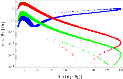
Figure 17: $\sigma\times\text{Br}$ for $pp\to\tilde{\chi}_{2}^{0}\>X\to\tilde{\chi}_{1}^{0}\>l\>l^{\prime}\>X$ as a function of $|\sin(\theta_{2}-\theta_{1})|$. The bands correspond to the following $l,l^{\prime}$ combinations: $e$ -$\mu$ (blue), $e$-$\tau$ (green) and $\mu$-$\tau$ (red). The parameters have been taken as in Figure 7. A center of mass energy of $14$ TeV has been assumed.

Up to now we have fixed the parameters such that Br$(\mu\to e\gamma)$ is close to its experimental bound. In the following we depart from this by performing a scan varying in particular $|\sin(\theta_{2}-\theta_{1})|$ because a strong dependence of the rare lepton decays on this quantity has been found, see Figure 7. In Figure 17 we show the rates for $pp\to\tilde{\chi}_{2}^{0}\>X\to\tilde{\chi}_{1}^{0}\>l\>l^{\prime}\>X$ as a function of $|\sin(\theta_{2}-\theta_{1})|$ for $\sqrt{s}=14$ TeV and fixing the parameters as in Figure 7. The final states containing a $\tau$-lepton behave similar as the corresponding rare $\tau$ decays. However, in case of the $e$-$\mu$ final state we find a lower limit of about 0.1 fb for this parameter set. The reason is, that above $|\sin(\theta_{2}-\theta_{1})|\simeq 0.3$ the mass splitting between the selectrons and smuons get smaller the larger $|\sin(\theta_{2}-\theta_{1})|$ is. This holds for both, left and right states. This leads to a decrease of Br$(\mu\to e\gamma)$ and at the same time to a slight increase of the lepton flavour violating signals at the LHC as can also be seen in Figure 18 where we show the LHC rate of the $e\mu$ final state as a function of Br$(\mu\to e\gamma)$.

In principle one might worry about the fact that the mass differences between the sleptons are partly smaller than the corresponding widths implying potential resonance effects ArkaniHamed:1996au ; ArkaniHamed:1997km . We have checked that the principal features discussed above remain if one does not use the narrow width approximation, leading to the cascades $\tilde{\chi}^{0}_{2}\to l\tilde{l}_{j}\to ll^{\prime}\tilde{\chi}^{0}_{1}$, but calculates the complete amplitudes using Breit-Wigner propagators for the sleptons. This shifts the results only very slightly.

Figure 18: $\sigma\times\text{Br}$ for $pp\to\tilde{\chi}_{2}^{0}\>X\to\tilde{\chi}_{1}^{0}\>e\>\mu\>X$ for $\sqrt{s}=14$ TeV as a function of Br($\mu\to e\gamma$) The parameters have been taken as in Figure 7. The vertical line shows the current MEG bound $\text{Br}(\mu\to e\gamma)<2.4\cdot 10^{-12}$.

VI Conclusions

We have studied phenomenological aspects of a supersymmetric left-right model. Our discussion has centered on two aspects: (a) Changes in the low energy SUSY spectra with respect to CMSSM expectations and the resulting consequences for the relic density of the lightest neutralino, assumed to be the cold dark matter of the universe. And (b) Lepton flavour violation induced by the LFV entries in the neutrino Yukawa coupling matrix, required to explain the observed neutrino angles, and consequences for the LHC.

In the CMSSM the lightest neutralino can have a relic density in agreement with the measured value Nakamura:2010zzi only in some very specific parts of parameter space. These well-known regions are (i) the stau co-annihilation region; (ii) stop co-annihilation region; (iii) the focus point line and (iv) the Higgs funnel. The modified running of the soft parameters in the $\Omega$LR model shifts the allowed regions. In general, the lower $v_{BL}$ and $v_{R}$ are, the smaller these regions become until for certain values of these parameters (depending on the specific region) the DM allowed regions disappear completely. From an observation of a SUSY spectrum consistent with any of these regions one could infer lower limits on $v_{BL}$ and $v_{R}$ not far below the GUT scale for CMSSM boundary conditions.

The model also allows for flavoured co-annihilation Choudhury:2011um . We have given some specific examples of parameter points in which it is possible to have large flavoured contributions to the co-annihilation cross section, despite the stringent upper limit on the decay $\mu\to e\gamma$ recently published by the MEG collaboration Adam:2011ch .

We have shown that LFV decays of the $\tilde{\chi}^{0}_{2}$ can reach up to 20 fb^-1 for the LHC at $\sqrt{s}=14$ TeV. All combinations of different lepton flavour final states could be large. These as well as the rare lepton decays show a strong dependence on the parameters of the model, noteworthy also on the high scale parameters $v_{R}$ and $\sin(\theta_{2}-\theta_{1})$.

Appendix A Invariants

Neglecting the contributions from the Yukawa couplings and working in the leading-log approximation, the soft mass parameters at the SUSY scale are computed to be

$$M_{i}(m_{SUSY})=\frac{\alpha_{i}(m_{SUSY})}{\alpha_{BL}(m_{GUT})}M_{1/2}$$ (27)

$$m_{f}^{2}=m_{0}^{2}+\frac{M_{1/2}^{2}}{\alpha_{BL}^{2}(m_{GUT})}\left[\alpha_{i}^{2}(v_{BL})f_{MSSM}^{i}+\check{\alpha}_{i}^{2}(v_{R})f_{BL}^{i}+\alpha_{i}^{2}(m_{GUT})f_{LR}^{i}\right]$$ (28)

In equ. (28) a sum over the index $i$ is implied, with $i=(Y,2,3)$ in the first and second terms and $i=(BL,2,3)$ in the third. The $f^{i}$ parameters are defined as

$$f_{MSSM}^{i} = \frac{B_{i}^{\tilde{f}}}{b_{MSSM}^{i}}\left[1-\left(\frac{\alpha_{i}(m_{SUSY})}{\alpha_{i}(v_{BL})}\right)^{2}\right]$$ (29)

$$f_{BL}^{i} = \frac{B_{i}^{\tilde{f}}}{b_{BL}^{i}}\left[1-\left(\frac{\alpha_{i}(v_{BL})}{\check{\alpha}_{i}(v_{R})}\right)^{2}\right]$$ (30)

$$f_{LR}^{i} = \frac{A_{i}^{\tilde{f}}}{b_{LR}^{i}}\left[1-\left(\frac{\hat{\alpha}_{i}(v_{R})}{\alpha_{i}(m_{GUT})}\right)^{2}\right]$$ (31)

For the numerical studies we have fixed the GUT scale to be $m_{GUT}=2\cdot 10^{16}$ GeV. The gauge couplings in the previous equations are determined by means of the general formula

$$\alpha_{i}(\mu_{2})=\alpha_{i}(\mu_{1})\left[1-\frac{\alpha_{i}(\mu_{1})}{4\pi}b^{i}\ln\left(\frac{\mu_{2}^{2}}{\mu_{1}^{2}}\right)\right]^{-1}$$ (32)

using the experimental values at $\mu=m_{Z}$ as starting point. In addition, at $\mu=v_{R}$ one must apply the following matching conditions

$$\hat{\alpha}_{BL}^{-1} = \frac{5}{2}\check{\alpha}_{Y}^{-1}-\frac{3}{2}\check{\alpha}_{2}^{-1}$$ (33)

$$\hat{\alpha}_{2} = \check{\alpha}_{2}$$ (34)

$$\hat{\alpha}_{3} = \check{\alpha}_{3}$$ (35)

In the previous three equations, the gauge couplings on the right-hand side are the ones for the $\mu<v_{R}$ regime, whereas the gauge couplings on the left-hand side are the ones for the $\mu>v_{R}$ regime.

The beta coefficients used in the previous formulas are

$$b^{SM} = (b_{Y}^{SM},b_{2}^{SM},b_{3}^{SM})=(\frac{41}{10},-\frac{19}{6},-7)$$ (36)

$$b^{MSSM} = (b_{Y}^{MSSM},b_{2}^{MSSM},b_{3}^{MSSM})=(\frac{33}{5},1,-3)$$ (37)

$$b^{BL} = (b_{Y}^{BL},b_{2}^{BL},b_{3}^{BL})=(\frac{33}{5},3,-3)$$ (38)

$$b^{LR} = (b_{1}^{LR},b_{2}^{LR},b_{3}^{LR})=(24,8,-3)$$ (39)

Finally, the $A_{i}^{\tilde{f}}$ and $B_{i}^{\tilde{f}}$ coefficients are

	$\displaystyle\tilde{e}^{c}$	$\displaystyle\tilde{L}$	$\displaystyle\tilde{d}^{c}$	$\displaystyle\tilde{u}^{c}$	$\displaystyle\tilde{Q}$
$A_{BL}$	$\displaystyle\frac{3}{4}$	$\displaystyle\frac{3}{4}$	$\displaystyle\frac{1}{12}$	$\displaystyle\frac{1}{12}$	$\displaystyle\frac{1}{12}$
$A_{2}$	$\displaystyle\frac{3}{2}$	$\displaystyle\frac{3}{2}$	$\displaystyle\frac{3}{2}$	$\displaystyle\frac{3}{2}$	$\displaystyle\frac{3}{2}$
$A_{3}$	$0$	$0$	$\displaystyle\frac{8}{3}$	$\displaystyle\frac{8}{3}$	$\displaystyle\frac{8}{3}$
$B_{Y}$	$\displaystyle\frac{6}{5}$	$\displaystyle\frac{3}{10}$	$\displaystyle\frac{2}{15}$	$\displaystyle\frac{8}{15}$	$\displaystyle\frac{1}{30}$
$B_{2}$	$0$	$\displaystyle\frac{3}{2}$	$0$	$0$	$\displaystyle\frac{3}{2}$
$B_{3}$	$0$	$0$	$\displaystyle\frac{8}{3}$	$\displaystyle\frac{8}{3}$	$\displaystyle\frac{8}{3}$

References

- (1) P. Minkowski, Phys. Lett. B 67 (1977) 421. T. Yanagida, in KEK lectures, ed. O. Sawada and A. Sugamoto, KEK, 1979; M Gell-Mann, P Ramond, R. Slansky, in Supergravity, ed. P. van Niewenhuizen and D. Freedman (North Holland, 1979);
- (2) R.N. Mohapatra, G. Senjanovic, Phys. Rev. Lett. 44 (1980) 912.
- (3) J. Schechter, J. W. F. Valle, Phys. Rev. D 22 (1980) 2227.
- (4) T. P. Cheng, L. F. Li, Phys. Rev. D 22 (1980) 2860.
- (5) J. C. Pati, A. Salam, Phys. Rev. D 10 (1974) 275 [Erratum-ibid. D 11 (1975) 703].
- (6) R. N. Mohapatra, J. C. Pati, Phys. Rev. D 11 (1975) 2558.
- (7) G. Senjanovic, R. N. Mohapatra, Phys. Rev. D 12 (1975) 1502.
- (8) R. N. Mohapatra, G. Senjanovic, Phys. Rev. D23 (1981) 165.
- (9) M. Cvetic, J. C. Pati, Phys. Lett. B 135 (1984) 57.
- (10) C. S. Aulakh, K. Benakli, G. Senjanovic, Phys. Rev. Lett. 79 (1997) 2188 [arXiv:hep-ph/9703434].
- (11) C. S. Aulakh, A. Melfo, A. Rasin, G. Senjanovic, Phys. Rev. D 58 (1998) 115007 [arXiv:hep-ph/9712551].
- (12) P. Fileviez Perez, S. Spinner, Phys. Lett. B 673 (2009) 251 [arXiv:0811.3424 [hep-ph]].
- (13) B. Brahmachari, E. Ma, U. Sarkar, Phys. Rev. Lett. 91 (2003) 011801 [arXiv:hep-ph/0301041].
- (14) F. Siringo, Eur. Phys. J. C 32 (2004) 555 [arXiv:hep-ph/0307320].
- (15) K. S. Babu, B. Dutta, R. N. Mohapatra, Phys. Rev. D60 (1999) 095004 [hep-ph/9812421].
- (16) For an introduction, see for example: M. Drees, R. Godbole, P. Roy, “Theory and phenomenology of sparticles: An account of four-dimensional N=1 supersymmetry in high energy physics,” Hackensack, USA: World Scientific (2004) 555 p
- (17) F. Borzumati, A. Masiero, Phys. Rev. Lett. 57 (1986) 961.
- (18) Super-Kamiokande collaboration, Y. Fukuda et al., Phys. Rev. Lett. 81 (1998) 1562; Q. R. Ahmad et al. [SNO Collaboration], Phys. Rev. Lett. 89 (2002) 011301; K. Eguchi et al. [KamLAND Collaboration], Phys. Rev. Lett. 90 (2003) 021802.
- (19) J. Hisano, T. Moroi, K. Tobe, M. Yamaguchi, T. Yanagida, Phys. Lett. B357 (1995) 579 [hep-ph/9501407].
- (20) J. Hisano, T. Moroi, K. Tobe, M. Yamaguchi, Phys. Rev. D53 (1996) 2442 [hep-ph/9510309].
- (21) J. N. Esteves, J. C. Romao, M. Hirsch, A. Vicente, W. Porod, F. Staub, JHEP 1012 (2010) 077 [arXiv:1011.0348 [hep-ph]].
- (22) Y. Kuno, Y. Okada, Rev. Mod. Phys. 73 (2001) 151 [arXiv:hep-ph/9909265].
- (23) M. Hirsch, S. Kaneko, W. Porod, Phys. Rev. D 78 (2008) 093004 [arXiv:0806.3361 [hep-ph]].
- (24) M. Hirsch, L. Reichert, W. Porod, JHEP 1105 (2011) 086 [arXiv:1101.2140 [hep-ph]]. Esteves:2010ff
- (25) J. N. Esteves, J. C. Romao, M. Hirsch, F. Staub, W. Porod, Phys. Rev. D83 (2011) 013003 [arXiv:1010.6000 [hep-ph]].
- (26) M. R. Buckley, H. Murayama, Phys. Rev. Lett. 97 (2006) 231801 [arXiv:hep-ph/0606088].
- (27) V. De Romeri, M. Hirsch, M. Malinsky, Phus. Rev. D, in press; [arXiv:1107.3412 [hep-ph]].
- (28) J. N. Esteves, S. Kaneko, J. C. Romao, M. Hirsch, W. Porod, Phys. Rev. D80 (2009) 095003 [arXiv:0907.5090 [hep-ph]].
- (29) C. Biggio, L. Calibbi, JHEP 1010 (2010) 037 [arXiv:1007.3750 [hep-ph]].
- (30) M. Drees, J. M. Kim, JHEP 0812 (2008) 095 [arXiv:0810.1875 [hep-ph]].
- (31) M. Drees, M. M. Nojiri, Phys. Rev. D 47 (1993) 376 [arXiv:hep-ph/9207234].
- (32) E. Komatsu et al., arXiv:1001.4538 [astro-ph.CO].
- (33) D. Choudhury, R. Garani, S. K. Vempati, arXiv:1104.4467 [hep-ph].
- (34) R. Kuchimanchi, R. N. Mohapatra, Phys. Rev. D 48 (1993) 4352 [arXiv:hep-ph/9306290].
- (35) R. Kuchimanchi, R. N. Mohapatra, Phys. Rev. Lett. 75 (1995) 3989 [hep-ph/9509256].
- (36) J. Kopp, M. Lindner, V. Niro, T. E. J. Underwood, Phys. Rev. D81 (2010) 025008 [arXiv:0909.2653 [hep-ph]].
- (37) S. Weinberg, Phys. Lett. B 91 (1980) 51.
- (38) B. A. Ovrut, H. J. Schnitzer, Nucl. Phys. B 179 (1981) 381.
- (39) L. J. Hall, Nucl. Phys. B 178 (1981) 75.
- (40) S. K. Majee, M. K. Parida, A. Raychaudhuri, U. Sarkar, Phys. Rev. D75 (2007) 075003 [hep-ph/0701109].
- (41) D. Borah, U. A. Yajnik, Phys. Rev. D83 (2011) 095004 [arXiv:1010.6289 [hep-ph]].
- (42) B. Holdom, Phys. Lett. B166 (1986) 196.
- (43) M. Malinsky, J. C. Romao, J. W. F. Valle, Phys. Rev. Lett. 95 (2005) 161801 [hep-ph/0506296].
- (44) R. Fonseca, M. Malinsky, W. Porod, F. Staub, Nucl. Phys. B 854 (2012) 28 [arXiv:1107.2670 [hep-ph]].
- (45) F. Staub, arXiv:0806.0538 [hep-ph].
- (46) F. Staub, Comput. Phys. Commun. 181 (2010) 1077 [arXiv:0909.2863 [hep-ph]].
- (47) F. Staub, Comput. Phys. Commun. 182 (2011) 808 [arXiv:1002.0840 [hep-ph]].
- (48) W. Porod, Comput. Phys. Commun. 153 (2003) 275 [arXiv:hep-ph/0301101].
- (49) W. Porod, F. Staub, arXiv:1104.1573 [hep-ph].
- (50) F. Staub, T. Ohl, W. Porod, C. Speckner, arXiv:1109.5147 [hep-ph].
- (51) V. Khachatryan et al. [CMS Collaboration], Phys. Lett. B698 (2011) 196 [arXiv:1101.1628 [hep-ex]].
- (52) G. Aad et al. [Atlas Collaboration], Phys. Rev. Lett. 106 (2011) 131802 [arXiv:1102.2357 [hep-ex]].
- (53) J. B. G. da Costa et al. [Atlas Collaboration], Phys. Lett. B 701 (2011) 186 [arXiv:1102.5290 [hep-ex]].
- (54) S. Chatrchyan et al. [CMS Collaboration], arXiv:1109.2352 [hep-ex].
- (55) Proposal to PSI: “MEG: Search for down to branching ratio”; Documents and status at http://meg.web.psi.ch/.
- (56) J. Adam et al. [MEG Collaboration], arXiv:1107.5547 [hep-ex].
- (57) W. Chao, Chin. Phys. C35 (2011) 214 [arXiv:0705.4351 [hep-ph]].
- (58) Y. Okada, K. -i. Okumura, Y. Shimizu, Phys. Rev. D61 (2000) 094001 [hep-ph/9906446].
- (59) J. Hisano, M. Nagai, P. Paradisi, Y. Shimizu, JHEP 0912 (2009) 030 [arXiv:0904.2080 [hep-ph]].
- (60) A. J. Buras, P. Gambino, M. Gorbahn, S. Jäger, L. Silvestrini, Phys. Lett. B500 (2001) 161 [hep-ph/0007085].
- (61) G. D’Ambrosio, G. F. Giudice, G. Isidori, A. Strumia, Nucl. Phys. B645 (2002) 155 [hep-ph/0207036].
- (62) K. Nakamura et al. [Particle Data Group Collaboration], J. Phys. G G37 (2010) 075021.
- (63) K. Griest and D. Seckel, Phys. Rev. D 43 (1991) 3191.
- (64) J. R. Ellis, T. Falk, K. A. Olive, Phys. Lett. B 444 (1998) 367 [arXiv:hep-ph/9810360].
- (65) C. Boehm, A. Djouadi, M. Drees, Phys. Rev. D62 (2000) 035012 [hep-ph/9911496].
- (66) J. R. Ellis, K. A. Olive, Y. Santoso, Astropart. Phys. 18 (2003) 395 [hep-ph/0112113].
- (67) J. Edsjo, M. Schelke, P. Ullio, P. Gondolo, JCAP 0304 (2003) 001 [arXiv:hep-ph/0301106].
- (68) J. L. Feng, K. T. Matchev, F. Wilczek, Phys. Lett. B482 (2000) 388 [hep-ph/0004043].
- (69) J. L. Feng, K. T. Matchev, T. Moroi, Phys. Rev. D61 (2000) 075005 [hep-ph/9909334].
- (70) J. R. Ellis, J. S. Hagelin, D. V. Nanopoulos, K. A. Olive, M. Srednicki, Nucl. Phys. B 238 (1984) 453.
- (71) G. Jungman, M. Kamionkowski, K. Griest, Phys. Rept. 267 (1996) 195 [arXiv:hep-ph/9506380].
- (72) G. Belanger, F. Boudjema, A. Pukhov, A. Semenov, Comput. Phys. Commun. 176 (2007) 367 [arXiv:hep-ph/0607059].
- (73) M. Hirsch, J. W. F. Valle, W. Porod, J. C. Romao, A. Villanova del Moral, Phys. Rev. D78 (2008) 013006 [arXiv:0804.4072 [hep-ph]].
-
(74)
F. Staub,
RGEs for Supersymmetric Left-Right Model, SARAH output,
http://theorie.physik.uni-wuerzburg.de/~fnstaub/Supplementary/Omega2.pdf - (75) B. C. Allanach, J. P. Conlon, C. G. Lester, Phys. Rev. D 77 (2008) 076006 [arXiv:0801.3666 [hep-ph]].
- (76) A. J. Buras, L. Calibbi, P. Paradisi, JHEP 1006 (2010) 042 [arXiv:0912.1309 [hep-ph]].
- (77) A. Abada, A. J. R. Figueiredo, J. C. Romao, A. M. Teixeira, JHEP 1010 (2010) 104 [arXiv:1007.4833 [hep-ph]].
-
(78)
B. O’Leary,
https://github.com/benoleary/LHC-FASER_light. - (79) W. Beenakker, R. Höpker, M. Spira, arXiv:hep-ph/9611232.
- (80) N. Arkani-Hamed, H. C. Cheng, J. L. Feng, L. J. Hall, Phys. Rev. Lett. 77 (1996) 1937 [arXiv:hep-ph/9603431].
- (81) N. Arkani-Hamed, J. L. Feng, L. J. Hall, H. C. Cheng, Nucl. Phys. B 505 (1997) 3 [arXiv:hep-ph/9704205].