Transversity studies with protons and light nuclei
Abstract
A general formalism to evaluate time-reversal odd transverse momentum dependent parton distributions (T-odd TMDS) is reviewed and applied to the calculation of the leading-twist quantities, i.e., the Sivers and the Boer-Mulders functions. Two different models of the proton structure, namely a non relativistic constituent quark model and the MIT bag model, have been used. The results obtained in both frameworks fulfill the Burkardt sum rule to a large extent. The calculation of nuclear effects in the extraction of neutron single spin asymmetries in semi-inclusive deep inelastic scattering off transversely polarized 3He is also illustrated. In the kinematics of JLab, it is found that the nuclear effects described by an Impulse Approximation approach are under theoretical control.
1 Introduction
The partonic structure of transversely polarized hadrons is still rather poorly known [1]. As a matter of facts, despite its leading-twist character, the transversity distribution is chiral-odd in nature and not accessible therefore in inclusive esperiments. Due to going-on and forthcoming important measurements in various Laboratories, this issue is nevertheless one of the most widely studied by the hadronic Physics Community, in particular by the Italian one, which is providing crucial contributions to a better understanding of this fascinating subject (see, for example, Refs. [2] and references therein).
Semi-inclusive deep inelastic scattering (SIDIS) is one of the proposed processes to access the parton structure of transversely polarized hadrons. The theoretical description of semi-inclusive processes implies a more complicated formalism, accounting for the transverse motion of the quarks in the target [3, 4, 5]. In particular, the non-perturbative effects of the intrinsic transverse momentum of the quarks inside the nucleon may induce significant hadron azimuthal asymmetries [6, 7].
The Sivers and the Boer-Mulders functions were defined in this scenario [8, 9]. Transverse Momentum Dependent pdfs (TMDs) are the set of functions that depend on the intrinsic transverse momentum of the quark, in addition to the dependences, typical of the PDs, on the Bjorken variable and on the momentum transfer . Their number is fixed counting the scalar quantities allowed by hermiticity, parity and time-reversal invariance. However, the existence of final state interactions (FSI) allows for time-reversal odd functions [10]. In effect, by relaxing this constraint, one defines two additional functions, namely, the Sivers and the Boer-Mulders (BM) functions. In SIDIS, the Sivers function is involved in the description of the single spin asymmetry, measured when an unpolarized beam scatters transeversely polarized targets. The single spin asymmetries are obtained constructing the difference of semi-inclusive cross-sections with different transverse polarization of the target with respect to the momentum transfer. The BM function appears in the azimuthal asymmetry in unpolarized SIDIS. The latter object refers to the detection of the produced hadron at different angles with respect to the plane containing the momentum transfer and the hadron momentum. All the involved quantities have been conventionally defined in Ref. [11]. According to the latter convention, the Sivers function, [8], and the Boer-Mulders function, [9], are formally defined through the following expressions111.:
| (1) | |||||
taking the proton polarized along the axis; and
| (2) | |||||
where is the spin of the target hadron. The normalization of the covariant spin vector is , is the target mass, is the quark field and is the gauge link.222The gauge link is defined as where is the strong coupling constant. This definition holds in covariant (non singular) gauges, and in SIDIS processes, as the definition of T-odd TMDs is process dependent. The gauge link contains a scaling contribution which makes the T-odd TMDs non vanishing in the Bjorken limit, as it has been shown in Refs. [12, 13, 14].
The difference between the two functions is clearly seen comparing Eq. (1) and Eq. (2). The BM function counts transversely polarized quarks, hence the Dirac operator in Eq. (2), in an unpolarized proton. On the other hand, the Sivers function counts the unpolarized quarks, hence the Dirac operator in Eq. (1), in a transversly polarized proton, denoted by the transverse component in the proton state in Eq. (1). If there were no scaling contribution of the gauge link, the two T-odd functions, and , would be identically zero.
2 Quark model calculations
Several quark model calculations of the Sivers and BM functions have been performed in the past years (see, i.e., Refs. [15, 16, 17, 18]) and their phenomenology keeps attracting interest, as it is demonstrated by very recent important contributions [19, 20, 21].
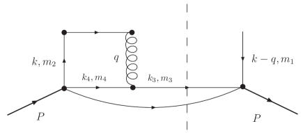
The general formalism for the evaluation of time-reversal odd TMDs in quark models, presented in Ref. [22, 23, 24], is reviewed here below. It is based on an impulse approximation analysis, where the Final State Interactions are introduced through a One Gluon Exchange mechanism, as depicted in Fig. 1. The used quark models, i.e., the simplest version of the MIT bag model [25], and a non relativistic constituent quark model (NRCQM), do not contain explicit gluonic degrees of freedom. In the Sivers and BM functions the Dirac operators determine the spin structure of the interaction, between the quarks with initial spins and and final spins and , respectively. For instance, in the MIT bag model [25], one gets, for the Sivers [BM] function
| (3) | |||||
The imaginary part is taken only for the Sivers function calculation, performed changing the transversely polarized nucleon states from a transversity to a helicity basis. The coupling of the spins at the quark level appears clearly from the expressions
| (4) | |||||
whose calculation has been performed assuming symmetry for the proton state, for . The interaction has been evaluated using the properly normalized fields for the quark in the bag [25], given in terms of the quark wave function in momentum space, which reads
| (5) |
with the normalization factor given in Ref. [25] The interaction is then
| (6) |
where or for, respectively, the Sivers and the Boer-Mulders function. The expressions in the NRCQM are similar to the one in the bag model. They read, being the intrinsic proton wave function,
where or for the BM and the Sivers function, respectively. The interaction here reads
| (8) |
with the four-spinor of the free quark states, arising from the Impulse Approximation analysis
In Refs. [22, 23, 24], the T-odd TMDs have been evaluated in both the MIT bag model and the NRCQM assuming initially an symmetry for the proton.
In the former case, the qualitative results are understood calculating the coefficients (4), in terms of which it is possible to realize what happens to the quark spins in the FSI process in a perfectly transparent way. In the latter case, one first has to re-express Eq. (LABEL:bm-cqm-ready) in terms of the proton state. In spectroscopic notation and with the Jacobi coordinates, one has, using SU(6) symmetry
| (9) |
where is the standard vector describing the spin-flavor structure of the proton. In the bag model calculation, a non-zero Sivers function arises through the interference between the upper and lower components of the wave function. Something similar happens in the CQM. This time the interference is between the upper and lower components of the free spinors appearing as a consequence of the use of the Impulse Approximation (see Eqs. (6, 8) for the interaction and Refs. [22, 23, 24] for details). Two different spin combinations contribute to the Sivers function. One of them comes from the spin-flipping of the quark interacting with the photon, i.e. the term in the MIT bag calculation
| (10) |
with a normalization factor, a weighting spin-flavor-color factor resulting from the matrix elements (4) and where include the momentum dependent part.333See Eqs. (8-9) of Ref. [23].
On the other hand, there are more spin combinations for the BM function.444See Eq. (13) of Ref. [24]. The first reason is that both non-flipping and double-flipping terms are important. The second reason is the sum over the two spin states, i.e. . Due to the spin-flavor-color coefficients, i.e., due to the symmetry assumption, the non-flipping term is more important than the double-flipping contribution. In effect, the latters are governed by the product of the two lower components of the bag wave function which encodes the most relativistic contribution arising in the MIT bag model. They turn out to be a few orders of magnitude smaller than the dominant ones, arising from the interference between the upper and lower parts of the bag wave function. This also happens if a proper non relativistic reduction of the gauge link, suitable for CQM calculations, is performed, justifying then the non relativistic approximation.
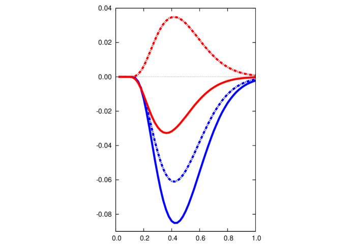
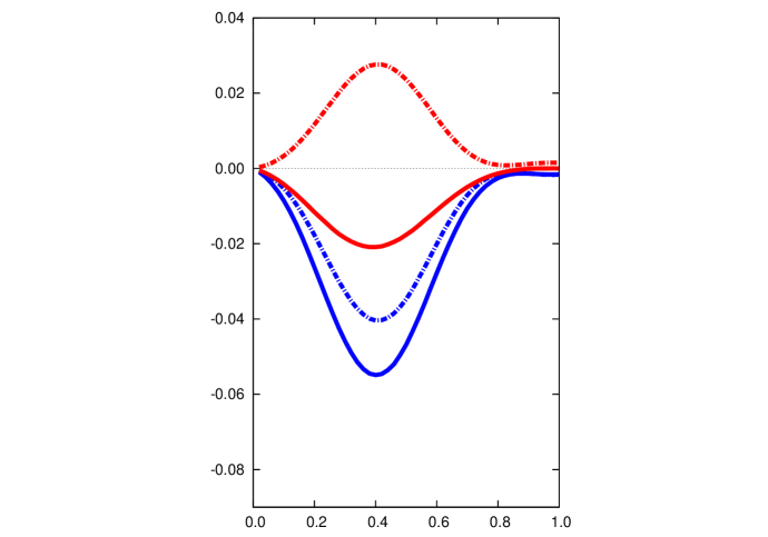
In Fig. 2 the “first moments” of the Sivers and the Boer-Mulders functions, i.e. the quantities
| (11) |
are shown for and quarks in both the CQM and MIT bag model, using [27].
x
x
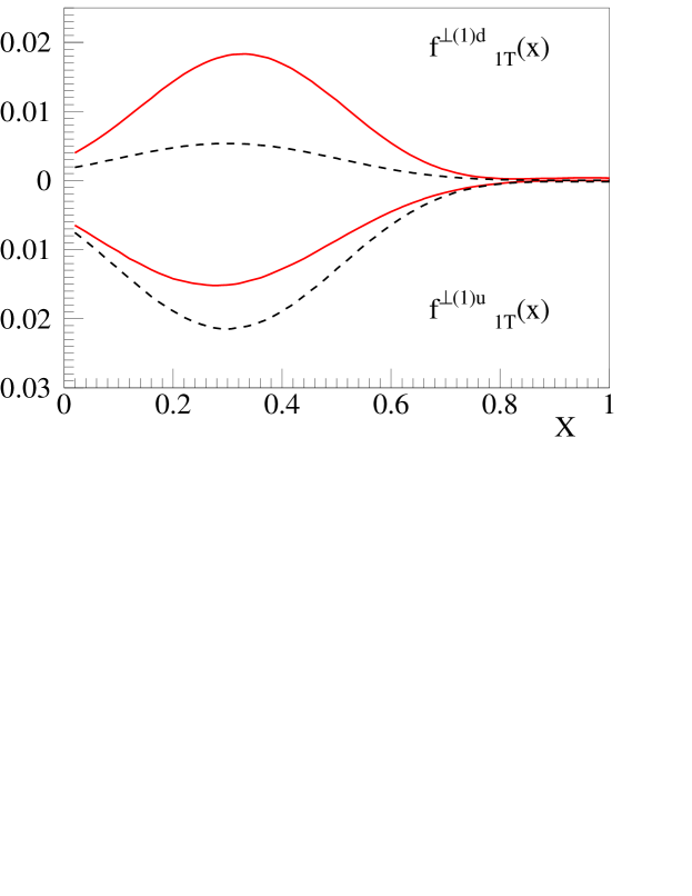
In Fig. 3 it is shown, in the MIT bag model case, the effect of neglecting the possible contribution of a spin-flip of the spectator quark (the one with initial spin projection in Fig. 1), as was done in a previous calculation [15]. The proper inclusion of this term is crucial for the fulfillment of the Burkart Sum Rule, as it is explained here below.
The above-described formalism has been easily extended, in the NR case, to the model of Isgur and Karl [26], allowing for a weak SU(6) breaking. The detailed procedure and the final expressions of the Sivers function in this model can be found in Ref. [22].

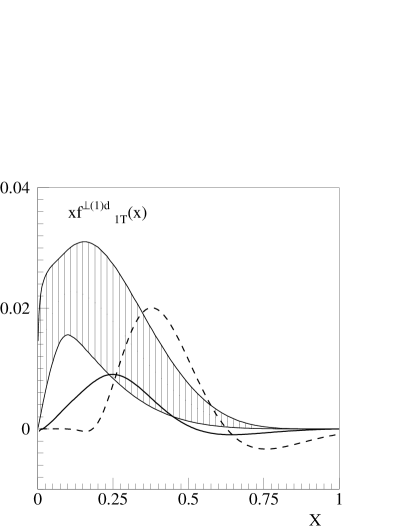
To evaluate numerically the Sivers and BM functions, the strong coupling constant (i.e. ) has to be fixed. The prescription of Ref. [27]. is used to fix , according to the amount of momentum carried by the valence quarks in the model. Here, assuming that all the gluons and sea pairs in the proton are produced perturbatively according to NLO evolution equations, in order to have of the momentum carried by the valence quarks at a scale of 0.34 GeV2 one finds that GeV2 if GeV. This yields [27]. The results of the present approach for the first moments of the Sivers function are given by the dashed curves in Fig. 4, where they are compared with a parameterization of the HERMES data, taken at GeV2. The patterned area represents the range of the best fit proposed in Ref. [28]. The results are close, in magnitude, to the data, although they have a different shape: the maximum (minimum) is predicted at larger values of . Actually is much lower, GeV2. For a proper comparison, the QCD evolution from the model scale to the experimental one would be necessary. Unfortunately, the Sivers function is a TMD PDs and the evolution of this class of functions is, to a large extent, unknown. In order to have an indication of the effect of the evolution, a NLO evolution of the model results has been performed, assuming, for , the same anomalous dimensions of the unpolarized PDFs. From the final result (full curve in Fig. 2), one can see that the agreement with data improves dramatically and the trend is reasonably reproduced at least for . Although the performed evolution is not exact, the procedure highlights the necessity of evolving the model results to the experiment scale and it suggests that the present results could be consistent with data, still affected by large errors. A discussion concerning the use of perturbative methods to relate the scale of model calculations to the scale of experimental data, and its impact on the calculation of T-odd TMDs, has been recently presented in Ref. [29] The deep understanding of the QCD evolution of TMDs is progressing fast [30, 31, 32, 33, 34].
Let us see now how the results of the calculation compare with the Burkardt sum rule [35], which follows from general principles. The Burkardt Sum Rule (BSR) states that, for a proton polarized in the positive direction, with
| (12) |
and must be satisfied at any scale. Within our scheme, at the scale of the model, it is found MeV, MeV and, in order to have an estimate of the quality of the agreement of our results with the sum rule, we define the ratio obtaining , so that one can say that the calculation fulfills the BSR to a precision of a few percent. One should notice that the agreement which is found is better than that found in previous model calculations, where the Sivers function for the flavor was found to be proportional to that for the flavor . For the MIT bag model, where the translational invariance is broken and the wave functions are not exact momentum eigenstates, the situatuion is slightly worse and the Sum Rule turns out to be violated of 5 % (one should realize anyway that, in a previous calculation without spin flip of the spectator quark, the violation was found to be 60 %).
The recent calculation of Ref. [18], using overlaps of Light Cone Wave Functions in the Light Front of Dynamics, where the number of particles and the momentum sum rules are satisfied at the same time, fulfills the Burkart Sume Rule exactly, showing the importance of using exact momentum eigenstates in checking the transverse momentum of the quarks.
3 The Sivers function from neutron (3He) targets
The experimental scenario which arises from the analysis of SIDIS off transversely polarized proton and deuteron targets is puzzling [36, 37].


With the aim at extracting the neutron information to shed some light on the problem, a measurement of SIDIS off transversely polarized 3He has been addressed [38], and an experiment, planned to measure azimuthal asymmetries in the production of leading from transversely polarized 3He, has been just completed at Jefferson Lab, with a beam energy of 6 GeV [39]. Another experiment will be performed after the 12 GeV upgrade of JLab [40, 41]. Here, a realistic analysis of SIDIS off transversely polarized 3He, presented in Ref. [42], is sommarized. The formal expressions of the Collins and Sivers contributions to the azimuthal Single Spin Asymmetry (SSA) for the production of leading pions off 3He have been derived, in impulse approximation (IA), including also the initial transverse momentum of the struck quark. The final equations are rather involved and they are not reported here. They can be found in [42]. The same quantities have been then evaluated in the kinematics of the planned JLab experiments. Wave functions [43] obtained within the AV18 interaction [44] have been used for a realistic description of the nuclear dynamics, using overlap integrals evaluated in Ref. [45], and the nucleon structure has been described by proper parameterizations of data [46] or suitable model calculations [47]. The crucial issue of extracting the neutron information from 3He data will be now thoroughly discussed. As a matter of facts, a model independent procedure, based on the realistic evaluation of the proton and neutron polarizations in 3He [48], called respectively and in the following, is widely used in inclusive DIS to take into account effectively the momentum and energy distributions of the polarized bound nucleons in 3He. It is found that the same extraction technique can be applied also in the kinematics of the proposed experiments, although fragmentation functions, not only parton distributions, are involved, as it can be seen in Figs. 5 and 6. In these figures, the free neutron asymmetry used as a model in the calculation, given by a full line, is compared with two other quantities. One of them is:
| (13) |
where stands for “Collins” or “Sivers”, is the result of the full calculation, simulating data, and is the neutron dilution factor. The latter quantity is defined as follows, for a neutron (proton ) in 3He:
| (14) |
and, depending on the standard parton distributions, , and fragmentation functions, , it is experimentally known (see [42] for details). is given by the dotted curve in the figures. The third curve, the dashed one, is given by
| (15) |
i.e. 3He is treated as a nucleus where the effects of its complicated spin structure, leading to a depolarization of the bound neutron, together with the ones of Fermi motion and binding, can be taken care of by parameterizing the nucleon effective polarizations, and . One should realize that Eq. (13) is the relation which should hold between the 3He and the neutron SSAs if there were no nuclear effects, i.e. the 3He nucleus were a system of free nucleons in a pure wave. In fact, Eq. (13) can be obtained from Eq. (15) by imposing and . It is clear from the figures that the difference between the full and dotted curves, showing the amount of nuclear effects, is sizable, being around 10 - 15 % for any experimentally relevant and , while the difference between the dashed and full curves reduces drastically to a few percent, showing that the extraction scheme Eq. (15) takes safely into account the spin structure of 3He, together with Fermi motion and binding effects. This important result is due to the peculiar kinematics of the JLab experiments, which helps in two ways. First of all, to favor pions from current fragmentation, has been chosen in the range , which means that only high-energy pions are observed. Secondly, the pions are detected in a narrow cone around the direction of the momentum transfer. As it is explained in [42], this makes nuclear effects in the fragmentation functions rather small. The leading nuclear effects are then the ones affecting the parton distributions, already found in inclusive DIS, and can be taken into account in the usual way, i.e., using Eq. (15) for the extraction of the neutron information. In the figures, one should not take the shape and size of the asymmetries too seriously, being the obtained quantities strongly dependent on the models chosen for the unknown distributions [47]. One should instead consider the difference between the curves, a model independent feature which is the most relevant outcome of the present investigation. The main conclusion is that Eq. (15) will be a valuable tool for the data analysis of the experiments [39, 40].
While the analysis of Ref. [42] has been performed assuming the experimental set-up of the experiment described in Ref. [39], but using DIS kinematics, a further analysis is being carried on [49], to investigate possible nuclear effects related to the finite values of the momentum and energy transfers, and , in the actual experiment. In Ref. [49], the description of Ref. [42] will be also improved, implementing a relativistic Light Front treatment to evaluate the nuclear polarized spectral function. Besides, the problem of possible effects beyond IA, such as final state interactions, will be addressed, and more realistic models of the nucleon structure, able to predict reasonable figures for the experiments, will be included in the general scheme.
Acknowledgments
I thank the organizers of the Conference for the kind invitation, A. Courtoy, F. Fratini and V. Vento for a fruitful and pleasent collaboration, A Del Dotto and G. Salmè for relevant discussions. This work is supported in part by the INFN-CICYT agreement.
References
References
- [1] Barone V, Drago A and Ratcliffe P 2002 Phys. Rept. 359 1
- [2] Ciullo G, Contalbrigo M, Hasch D, Lenisa P 2009 Proc. of the Second Workshop on Transverse Polarizatin Phenomena in Hard Processes, “Transversity 2008”, Ferrara, Italy, 28-31 May 2008, (Singapore: World Scientific).
- [3] Bacchetta A, Diehl M, Goeke K, Metz A, Mulders P.J. and Schlegel M 2007 J. High Energy Phys. JHEP 0702 093
- [4] D’Alesio U and Murgia F 2008 Prog. Part. Nucl. Phys. 61 394
- [5] Pasquini B, Cazzaniga S and Boffi S 2008 Phys. Rev. D 78 034025
- [6] Mulders P.J. and Tangerman R.D. 1996 Nucl. Phys. B 461 197 [Erratum-ibid. 1997 B 484 538]
- [7] Cahn R. N. 1978 Phys. Lett. B 78 269
- [8] Sivers D.W. 1990 Phys. Rev. D 41 83; 1991 Phys. Rev. D 43 261
- [9] Boer D. and Mulders P.J. 1998 Phys. Rev. D 57 5780
- [10] Brodsky S J, Hwang D S and Schmidt I 2002 Phys. Lett. B 530 99
- [11] Bacchetta A, D’Alesio U, Diehl M and Miller C A 2004 Phys. Rev. D 70 117504
- [12] Brodsky S J, Hoyer P, Marchal N, Peigne S and Sannino F 2002 Phys. Rev. D 65 114025
- [13] Collins J C 2002 Phys. Lett. B 536 43
- [14] Belitsky A V, Ji X and Yuan F 2003 Nucl. Phys. B 656 165
- [15] Yuan F 2003 Phys. Lett. B 575 45
- [16] Gamberg L.P., Goldstein G.R. and Schlegel M 2008 Phys. Rev. D 77 094016
- [17] Bacchetta A, Conti F and Radici M 2008 Phys. Rev. D 78 074010
- [18] Pasquini B and Yuan F 2010 Phys. Rev. D 81 114013
- [19] Barone V, Melis S and Prokudin A 2010 Phys. Rev. D 81 114026
- [20] Boer D 2011 On a possible node in the Sivers and Qiu-Sterman functions Preprint arXiv:1105.2543 [hep-ph]
- [21] Bacchetta A and Radici M 2011 Constraining quark angular momentum through semi-inclusive measurements Preprint arXiv:1107.5755 [hep-ph]
- [22] Courtoy A, Fratini F, Scopetta S and Vento V 2008 Phys. Rev. D 78 034002
- [23] Courtoy A, Scopetta S and Vento V 2009 Phys. Rev. D 79 074001
- [24] Courtoy A, Scopetta S and Vento V 2009 Phys. Rev. D 80 074032
- [25] Jaffe R L 1975 Phys. Rev. D 11 1953
- [26] Isgur N and Karl G 1978 Phys. Rev. D 18 4187; 1979 Phys. Rev. D 19 2653 [Erratum-ibid. 1981 D 23 817 ]
- [27] Traini M, Mair A, Zambarda A and Vento V 1997 Nucl. Phys. A 614 472
- [28] Efremov A V, Goeke K, Menzel S, Metz A and Schweitzer P 2005 Phys. Lett. B 612 233; Collins J C, Efremov A V, Goeke K, Menzel S, Metz A and Schweitzer P 2006 Phys. Rev. D 73, 014021
- [29] Courtoy A Scopetta S and Vento V 2011 Eur. Phys. J. A 47 49
- [30] Ceccopieri F A and Trentadue L 2008 Phys. Lett. B 660 43
- [31] Kang Z B and Qiu J W 2009 Phys. Rev. D 79 016003
- [32] Zhou J Yuan F and Liang Z T 2009 Phys. Rev. D 79 114022
- [33] Vogelsang W and Yuan F 2009 Phys. Rev. D 79 094010
- [34] Cherednikov I O, Karanikas A I and Stefanis N G 2010 Nucl. Phys. B 840 379
- [35] Burkardt M 2004 Phys. Rev. D 69 091501; Phys. Rev. D 69 057501
- [36] Airapetian A et al. [HERMES Collaboration] 2005 Phys. Rev. Lett. 94 012002
- [37] Alexakhin V Y et al. [COMPASS Collaboration] 2005 Phys. Rev. Lett. 94, 202002
- [38] Brodsky S J and Gardner S 2006 Phys. Lett. B 643 22
- [39] Qian X et al. 2011 Single Spin Asymmetries in Charged Pion Production from Semi-Inclusive Deep Inelastic on a Transversely Polarized 3He Target Preprint arXiv:1106.0363v3 [nucl-ex]
- [40] Gao H et al. 2011 Eur. Phys. J. Plus 126, 2
- [41] Del Dotto A., Master Thesis, Università di Roma “La Sapienza”, 2011 (unpublished).
- [42] Scopetta S. 2007 Phys. Rev. D 75 054005
- [43] Kievsky A, Viviani M and Rosati S 1994 Nucl. Phys. A 577 511
- [44] Wiringa R B, Stocks V G J and Schiavilla R 1995 Phys. Rev. C 51 38
- [45] Kievsky A, Pace E, Salmè G, and Viviani M 1997 Phys. Rev. C 56 64 Pace E, Salmè G, Scopetta S and Kievsky A 2001 Phys. Rev. C 64 055203
- [46] Anselmino M, Boglione M, D’Alesio U, Kotzinian A, Murgia F and Prokudin A 2005 , Phys. Rev. D 71 074006; 2005 Phys. Rev. D 72 094007 [2005 Erratum-ibid. D 72 099903].
- [47] Amrath D, Bacchetta A and Metz A 2005 Phys. Rev. D 71 114018
- [48] Ciofi degli Atti C, Scopetta S, Pace E and Salmè G 1993 Phys. Rev. C 48 968
- [49] Del Dotto A, Salmè G and Scopetta S, in preparation.