1 Introduction
While doing perturbation analysis and studying structure formation
process, if we use conventional tensoral method, it is difficult to
linearize Eistein’s equation. Even if it is linearized, it is not
easy to get the solutions and fully interpret them . Some of the informations
are lost in the process of linearizations. All these problems are
solved and the solutions are obtained in more natural ways if we use
Newman-Penrose (NP) formalism. In NP formalism, the unperturbed /
background quantities vanish and the equations left behind are in
terms of perturbed quantities only. So, it is more natural in analysing
the perturbation and structure formation.
The Newman-Penrose[1] formalism of projecting vectors, tensors
and spinors onto a set of null tetrad bases has proved to be an immensely
useful tool to investigate the properties of quantum fields in curved
spacetime. It has been used successfully in various black hole geometries
[2, 3, 4, 5, 6, 7, 8, 9, 10, 11].
The method has also been used more recently[12]
to further study the behaviour of Dirac particles in different geometries.
As the geometry of our Universe is of the Friedmann-Robertson-Walker
type, it is important to study how electrodynamics is altered by the
real expanding Universe in contrast to that in Minkowskian spacetime.
The behaviour of the quantum fields in FRW spacetime must be indicative
of the exact nature of the geometry of our Universe, particularly
whether it is flat, closed or open. Properties of matter fields in
general, and the massive Dirac fields in particular, must have profound
consequences on the structure formation process. Propagation of electromagnetic
waves in FRW spacetime was studied by Haghighipour[13] (see
references therein), among other authors. The Dirac field was studied
in the NP formalism by Zecca[14, 15] and the work
was continued further by Sharif[16].
Motivated by the success of the Newman-Penrose(NP) method in investigating
the perturbation of various black hole geometries, we thought that
the application of this method to study the perturbation of the Friedmann-Robertson-Walker
spacetime may give some further insight into structure formation.
One of the authors [17, 18] had used this formalism to study
free Maxwell and Dirac fields in FRW space. After setting up the notations
below, we write down the perturbation equations in the next section
and solve them. Section 3 discusses the scalar perturbation, and the
Green’s function as well as the Lienard-Wiechert type potential in
closed space are found. In the final section we discuss some consequences.
Writing the line element as [19, 20]
|
|
|
(1) |
with , we may devise
the null tetrad to be
and the complex conjugate to express the directional
derivatives as
|
|
|
|
|
|
|
|
|
|
(2) |
with
and .
Also, the non-vanishing spin coefficients[21] are given
by
|
|
|
(3) |
where the overdot and prime denote derivatives with the conformal
time and respectively.
Of the NP quantities representing the curvature of the spacetime,
all the Weyl scalers vanish in the homogeneous
and isotropic FRW background, and the non-vanishing background Ricci
scalers are given through
|
|
|
|
|
|
|
|
|
|
(4) |
In the work below, we just consider the closed Universe with ,
as the other two, turn out to be analytic continuation
of the same solution.
We will also have to use the operators
and .
2 Perturbation of the space-time
Now we look at the perturbation equations. In combination with the
’s that vanish in the background, we should take the unperturbed
directional derivatives and spin coefficients for the first order
perturbation equations. These equations are given by
|
|
|
|
|
|
|
|
|
|
|
|
|
|
|
|
|
|
|
|
|
|
|
|
|
|
|
|
|
|
|
|
|
|
|
|
|
|
|
|
where the explicit terms in the Ricci tensors (enclosed in square
brackets) are found on page 50 of Ref. [21]. The letters
(a), (b), etc. correspond to those equations there.
All these can be combined in one master equation:
|
|
|
(6) |
|
|
|
(7) |
representing the gravitational or tensorial perturbations,
|
|
|
(8) |
representing the vectorial or vortical perturbations, and
|
|
|
(9) |
the scalar perturbations. The sources are given by which
can be identified as
|
|
, |
|
|
|
|
, |
|
|
|
|
, |
|
|
|
|
, |
|
|
Although Eq. (6) appears to be valid for massless
spin fields of all helicities, we can define the source term only
for . To decouple the spin fields in Eq. (6),
we consider the Eq. (6) with ,
interchanging the upper and lower signs to get
|
|
|
(11) |
Then operating on Eq. (6) with
and Eq. (11) with
and adding the two, we find
|
|
|
|
|
(12) |
|
|
|
|
|
The equations for the vectorial perturbations are the same as the
Maxwell equations discussed in Ref.[17]. It is an interesting
proposition that the vortical perturbations arise from the electrodynamic
interaction between the Maxwell and Dirac fields. Simlarly, the equation
governing the scalar perturbation is the same as that of the conformally
coupled massless Klein-Gordon field. There are degrees of gauge
freedom in the problem as we have formulated, four relating to the
general co-variance of general relativity and six corresponding to
rotations of the tetrad frame as discussed in Ref. [21].
These conditions can best be used to simplify the source term, but
we will not be concerned with the sources in this work, and will only
discuss the eigen-modes of these perturbations.
It is clear that the angular part is separable, and we may write .
The eigenequations for are represented by the the spin-weighted
spherical harmonics satisfying
|
|
|
|
|
(13) |
|
|
|
|
|
(14) |
the solution[22] is
|
|
|
(15) |
allowing us to identify the spin-weighted spherical harmonics as the
spherical harmonics formed with the Jacobi polynomial .
It can easily be established that ,
and are just the usual spherical harmonics.
These are normalized to give ,
and they form a complete set in that ()=(-’).
Koornwinder[23] developed an addition formula for Jacobi
polynomials, and there is a generalized addition theorem for
given in Ref.[24], but we can devise a degenerate form for our
purpose by noting that can depend
only on the angle between the directions
where
|
|
|
(16) |
So, multiplying (-’)=
on both sides by and integrating
over the solid angle to find ,
we may write
|
|
|
(17) |
For the radial eigenfunctions, we substitute .
With a change of variable , we find
which looks the same as the angular operator. Hence
|
|
|
(18) |
where
|
|
|
|
|
(19) |
is the normalization constant, and the parameters of the Jacobi
polynomials are chosen to make the function regular at .
Ref. [25] has proved the non-Hermitian orthogonality of
Jacobi polynomials with general parameters. In our case, we find that
gives us
|
|
|
(20) |
So It should be noted
that and R are not orthogonal.
Both the angular and radial functions satisfy the spin raising and
lowering operations
|
|
|
|
|
|
|
|
|
|
(21) |
where the eigenvalues are
and .
In Eq. (21), the upper signs lower the helicity while the
lower signs raise it. Also the eigen-values satisfy .
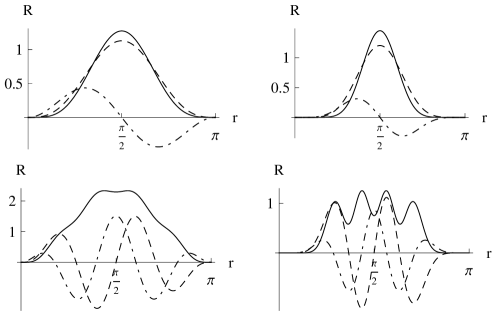
Some of the eigen-functions representing the various modes of perturbation
are displayed in the accompanying figures. The scalar perturbations,
Fig. (1), represent the density perturbations. These give
rise to the structures. Fig. (2) show the vectorial perturbations.
These are responsible for generating rotational or vortical effects
of the perturbations. The next mode shown in Fig. (3)
are the tensorial perturbation representing the gravitational radiation
content. All these modes are inter-related; e.g., any scalar density
enhancement due to gravitational collapse generates a rotational component
and induces the release of binding energy through gravitational radiation.
In future work, it will be important to solve the equations with the
source as well. The source terms are generated by products of these
eigenfunctions. For example, the source is generated
by products like .
The radial and temporal parts of the spin field wave of helicity p
are given by .
When two such waves of and are combined, the combination
must have helicity ; energy conservation (orthogonality
of the temporal part) requires and
the combined state must be linear superposition of the available momentum
states. So we can write
|
|
|
(22) |
The Clebsch-Gordon type coefficient can be determined to
be
|
|
|
(23) |
Triple integrals for conventional Jacobi polynomials have been considered
in the literatures [31] by using group theoritical
method. Here, we derive the Clebsch-Gordan type coefficients by direct
integration. So it is worthwhile to consider the product .
Clebsch-Gordan expansion of the product of the angular function is
well known:
|
|
|
|
|
|
|
|
|
|
(24) |
where
is the Clebsch-Gordan coefficient, , ,
. Here we will develop
a similar expansion for z.
With , and ,
substituting the Rodrigue’s formula for the Jacobi polynomial in the
first part of the integrand of Eq. (23) and integrating
by parts k times (with the integrated part vanishing at the boundary),
we find
|
|
|
|
|
|
|
|
(25) |
Using and the Leibniz rule, we have
|
|
|
|
|
|
(30) |
|
|
|
|
|
|
(35) |
|
|
|
(38) |
Substituting these expressions and further integration by parts gives
|
|
|
|
|
|
|
|
|
|
|
|
|
|
|
|
|
|
|
|
|
|
|
|
|
(51) |
|
|
|
|
|
Since ,
we have
|
|
|
|
|
|
|
|
|
|
|
|
|
|
|
|
|
|
|
|
(54) |
So, combining Equations (51) and (54), we
get
|
|
|
|
|
(69) |
|
|
|
|
|
|
|
|
|
|
|
|
|
|
|
3 Scalar Perturbation
Let us look at the scalar perturbation in some greater detail. To
solve the inhomogeneous equation with source, we can work out the
Green’s function by writing Eq. (11) for with
the delta function source[26]:
|
|
|
(70) |
The temporal eigen-functions are , the angular
are the spherical harmonics and the radial
ones are the normalized and appropriately weighted Gegenbauer polynomial
. Now we can immediately
write down the eigen-function expansion of the Green’s function [27]
as
|
|
|
|
|
(71) |
|
|
|
|
|
Firstly, the integral over can be done by the method of
residues to give
|
|
|
(72) |
Next, the addition theorem for spherical harmonics can be used to
write
|
|
|
(73) |
where is the angle between the directions .
Then we are left with
|
|
|
|
|
(74) |
|
|
|
|
|
Here, we may use the addition theorem for Gegenbauer polynomials[28]
to replace the second summation with
|
|
|
(75) |
where . Thus,
|
|
|
|
|
(76) |
|
|
|
|
|
The first term within the braces is the retarded, and the second is
advanced, Green’s function. In the limit to the flat case ,
we find , and ;
hence we recover the familiar Green’s function from classical electrodynamics.
With Eq. (76), we can consider the potential
of a point scalar perturbation moving along the trajectory
to find a retarded Lienard-Wiechert type potential. Thus,
|
|
|
|
|
(77) |
|
|
|
|
|
The integral over can now be easily done to give
|
|
|
(78) |
where the variables are to be evaluated at the retarded time ;
here,
|
|
|
(79) |
|
|
|
(80) |
with the primed co-ordinates being the location of the source that
produce the potential at the un-primed location of the observer; also
the right hand side is to be evaluated at the retarded time. Without
loss of generality, we may simplify the notation by locating the observer
at the origin, in which case .
Again it can be easily checked that Eq. (78) reduces to the
familiar form in the limit .
4 Relation to metric perturbation: application to shearing
The perturbed tetrad is written as a superposition of the unperturbed
ones viz., where
are first order in perturbation and
and the superscript indicates first order in perturbation.
are real
and others complex with the interchange of indices
given the complex cojugate. Hence 16 real functions are required to
specify all . These are subject to 10 gauge freedoms,
4 of general covariance and 6 of tetrad rotations.
The Ricci identities provide the equations satisfied by the spin coefficients.
In particular, the one that relates the shear to the gravitational
radiation is ([21], Eq. 8.310 b)
|
|
|
(81) |
Using the boost and spin weight raising and lowering operators ( and ),
we are just able to read off the solutions
|
|
|
(82) |
|
|
|
(83) |
To relate the spin coefficients to we need to linearize
the commutation relation
to first order in perturbation by writing
to get
|
|
|
(84) |
where are the directional derivatives. For our purpose
the two important ones are
|
|
|
(85) |
|
|
|
(86) |
Now Eqs. (82) and (85) can be used together
to get
|
|
|
(87) |
|
|
|
(88) |
With Eqs. (83) and (86), we find
and
|
|
|
(89) |
Next, using similar Ricci identities for and , and
the related structure constants, we find
|
|
|
(90) |
|
|
|
(91) |
|
|
|
(92) |
With these solutions, we can now determine some of the components
of the perturbed metric tensor given by
|
|
|
(93) |
|
|
|
(94) |
relates the gravitational radiation through shearing to the ()
component of the metric tensor. It is well known that the universe
contains a background gravitational radiation at a temperatureod ~
0.91K [29]. It is clear that this produces a shearing
which will distort the geometry of space time. We further find that
. Similarly,
|
|
|
|
|
(95) |
|
|
|
|
|
which will generate a perturbation in the radial velocity of matter.
There also appears a peculiar transverse motion generated by
|
|
|
(96) |
We are able to solve for 12 out of 16 real functions required to describe
the perturbed metric without using gauge conditions, leaving the four
real functions and to
be determined. For these, we will have to include the matter producing
the perturbation. In other works, we have solved the Dirac[30]
as well as Maxwell equations. The matter sources are related to the
spin coefficients by other Ricci identities like
|
|
|
|
|
(97) |
|
|
|
|
|
|
|
|
|
|
which is used to derive the optical theorem. In the perturbing source
, we have to include the energy-momentum of the
Maxwell, Dirac, their interactions, etc. It should be noted that the
RHS of last equation mostly represent second order quantities in the
perturbations. The real part of is the compression while
its imaginary part is the rotation.