Distributed Algorithms for Consensus and Coordination in the Presence of Packet-Dropping Communication Links
Part I: Statistical Moments Analysis Approach

Abstract

This two-part paper discusses robustification methodologies for linear-iterative distributed algorithms for consensus and coordination problems in multicomponent systems, in which unreliable communication links may drop packets. We consider a setup where communication links between components can be asymmetric (i.e., component $j$ might be able to send information to component $i$, but not necessarily vice-versa), so that the information exchange between components in the system is in general described by a directed graph that is assumed to be strongly connected. In the absence of communication link failures, each component $i$ maintains two auxiliary variables and updates each of their values to be a linear combination of their corresponding previous values and the corresponding previous values of neighboring components (i.e., components that send information to node $i$). By appropriately initializing these two (decoupled) iterations, the system components can asymptotically calculate variables of interest in a distributed fashion; in particular, the average of the initial conditions can be calculated as a function that involves the ratio of these two auxiliary variables. The focus of this paper to robustify this double-iteration algorithm against communication link failures. We achieve this by modifying the double-iteration algorithm (by introducing some additional auxiliary variables) and prove that the modified double-iteration converges almost surely to average consensus. In the first part of the paper, we study the first and second moments of the two iterations, and use them to establish convergence, and illustrate the performance of the algorithm with several numerical examples. In the second part, in order to establish the convergence of the algorithm, we use coefficients of ergodicity commonly used in analyzing inhomogeneous Markov chains.

I Introduction

The design of protocols and algorithms for distributed computation and control/decision tasks has attracted significant attention by the computer science, communication, and control communities (e.g., [1, 2, 3, 4, 5, 6, 7] and references therein). For example, given i) a collection of robots moving in the plane, ii) a collection of sensors in a sensor network, or iii) a collection of distributed energy resources in an electrical grid, the components may be interested in, respectively, i) agreeing on a common direction to follow (this common direction could be provided by a leader robot), ii) measurement averaging (with each sensor providing a local measurement of a global quantity), or iii) collectively providing a predetermined total amount of active power subject to the constraints of each distributed resource. In the control literature, the first and second problems are respectively known as consensus and average consensus (see, e.g., [2]), whereas the third problem can be considered as a distributed resource coordination problem [8, 9].

In this two-part paper, we consider multicomponent systems in which each component can exchange information with other components in its neighborhood in order to compute, in a distributed fashion, some quantity of interest. In our setup, communication links between components (nodes) can be asymmetric (i.e., component $j$ might be able to send information to component $i$, but not necessarily vice-versa), a situation that arises in a wireless setting if the transmission power available to different nodes are also different. In this setting, the information exchange between components in the system can be described by a directed graph which is assumed to be strongly connected. Through an iterative process, nodes in the network are required to compute (using only information made available by their neighbors) the quantity of interest. In particular, we study linear-iterative algorithms in which each node $j$ maintains a value (or a set of values) that is updated to be a weighted linear combination of node $j$’s own previous value and the previous values of its neighboring nodes (i.e., nodes that transmit information to node $j$). The main focus of the paper is to develop strategies to robustify the linear-iterative algorithms described above against communication links that may drop packets.

In the context of consensus and average-consensus problems, an extensive literature in the control community focuses on the linear-iterative algorithms described above (e.g., [7, 10, 2, 11, 12, 13, 14] and references therein). These works have revealed that if the network topology satisfies certain conditions, the weights for the linear iteration can be chosen so that all the nodes asymptotically converge to the same value (even if the network connections are time-varying). Additionally, if the interconnection topology is invariant and bidirectional (i.e., if node $j$ can send information to node $i$, then node $i$ can send information to node $j$), simple techniques can be used to choose the weights of the linear iteration so as to ensure that, after running the linear iteration, the nodes will asymptotically reach consensus to the average of their initial values [2, 11, 12]. Other works have looked at the consensus and average-consensus problems when the interconnection topology is described by a directed graph. In particular, the authors of [15] focus on continuous-time linear iterations and state necessary and sufficient conditions for a network of integrators to asymptotically reach agreement to a common value (but not necessarily the average of their initial values). Similarly, the authors of [12] consider discrete-time iterations, and provide necessary and sufficient conditions on the weights that allow the nodes to asymptotically reach consensus to the average of their initial values. Additionally, the work in [16, 17] discusses how average-consensus can be reached asymptotically with linear-iterative algorithms in which the nodes use fixed weights in their linear updates and also develops linear-iterative algorithms where the nodes adapt their weights in a distributed fashion so that asymptotically average-consensus is reached. In the context of resource coordination, there is some recent work [18, 8, 9] that also focuses on linear-iterative algorithms, similar to those used to address consensus and average-consensus problems. Other recent work has addressed the related problem of achieving consensus and average-consensus in a multicomponent system where some nodes can exhibit malicious behavior [19, 20]. These works assume fault-free communication links, but are related to what we do in this paper in the sense that they can be used to handle unreliable nodes (as opposed to links).

In our development, we adopt a very general model for the communication modality between nodes, which allows asymmetric information structures, in the sense that if node $i$ can transmit information to another node $j$, it is not necessarily true that node $j$ can transmit information to node $i$. We only require that each node, apart from seeing incoming transmissions sent to it by neighboring nodes, knows the number of nodes that it can transmit information to, which in graph-theoretic terms is referred to as the out-degree of that node. In fact, in the proposed algorithm, each node will broadcast the same quantity to all receiving nodes, which simplifies the communication scheme between sending and receiving nodes (as it is not necessary for each sending node to separately communicate with each receiving node).

When the communication network is perfectly reliable (no packet drops), the collective dynamics of the linear iterations can be described by a discrete-time transition system with no inputs in which the transition matrix is column stochastic and primitive. Then, each node will run two identical copies of the linear iteration each of which, however is initialized differently depending on the problem to be solved.In this paper we mostly focus on the average consensus problem. Under proper initialization, it can be shown that each node will asymptotically calculate the desired value as a function of the outcomes of the two iterations. The details of these double-iteration approach are provided in [16, 17] for the average consensus case and in [8, 9] for the resource coordination problem. For the average-consensus problem, the double-iteration algorithm is a particular case of the algorithm in [21] (which is a generalization of the algorithm proposed in [22]), where the matrices describing each linear iteration are allowed to vary as time evolves, whereas in our setup (for the ideal case when there are no communication link failures) the transition matrix is fixed over time.

The focus of this paper is to robustify the double-iteration algorithm (informally described above and formally described in Section II) so that it can tolerate failures in communication links and converge to the average value. Our communication link reliability model assumes that at each time step, a communication link is unavailable with some probability. In other words, a packet containing information from node $i$ to node $j$ is dropped with some probability. Next we informally describe our robustification approach. Consider two nodes $i$ and $j$, and assume that $j$ receives information from node $i$ but not necessarily vice-versa. Let us refer to $j$ as the receiving node (or receiver) and $i$ as the sending node (or sender). An important requirement is for the graph describing the communication network to be strongly connected, which implies every node must be able to act both as a sender and as a receiver. Then, for each of the two iterations each node performs, node $i$ (the sender) will keep track of the following quantities of interest: i) its own internal state (as captured by the state variables maintained in the double iteration scheme of [21, 18]; ii) the total mass broadcasted so far (to be described in detail soon); and iii) the total received mass from each node $l$ that sends information to node $i$. Similarly, for both iterations, each node $j$ (the receiver) updates the value of its internal state to be a linear combination of its own previous internal state value (weighted by the inverse of the number of nodes that have $j$ as a neighbor) and the difference between the two most recently received mass values from each of its neighbors (also weighted by the inverse of the number of nodes that have $j$ as a neighbor). At time instant $k$, the total broadcasted mass by node $j$ is the sum up to (and including) time step $k$ of the sequence of values of node $j$’s internal value, weighted by the inverse of the number of nodes that receive values from node $j$). Additionally, node $j$ updates the value of the received mass from each node $l$ that sends information to node $j$ as follows: the received mass from node $l$ is the total broadcasted mass sent by node $l$ up to time $k$ if the communication link from node $l$ to node $j$ is available at time step $k$; otherwise, the received mass remains the same as the most recently received mass from node $l$. An implicit assumption here is that messages broadcasted by node $l$ are tagged with the sender’s identity so that the receiving node $j$ can determine where different packages have originated from.

Recent work that has addressed the consensus and average-consensus problems in the presence of unreliable communication links [23, 24, 25] has employed a communication link availability model similar to ours. The work in [23] assumes that the graph describing the communication network is undirected and that when a communication link fails it affects communication in both directions. Additionally, nodes have some mechanism to detect link unavailability and compensate for it by rescaling their other weights (so that the resulting transition matrix remains column stochastic). Following this strategy, the authors show asymptotic convergence to the average of initial conditions and also calculate the rate at which the variance of the total deviation from the average converges to zero. The work in [24] does not require the graph describing the communication network to be undirected and proposes two compensation methods to account for communication link failures. In the first method, the so-called biased compensation method, the receiving node compensates for the unavailability of an incoming link by adding the weight associated to the unavailable link to its own weight (so that the resulting matrix remains row stochastic). In the second method, called the balanced compensation method, the receiving node compensates for link unavailability by rescaling all the incoming link weights so that the resulting matrix remains row stochastic. The key in both methods is the fact that at each time step, the resulting weight matrix is row stochastic; the authors show that the nodes converge almost surely to the same value, but this value is not necessarily the average of the initial conditions. The work in [25], which does not require the communication graph to be undirected, proposes a correction strategy that corrects the errors in the quantity (state) iteratively calculated by each node, so that the nodes obtain the average of their initial values. This correction strategy is based on each node maintaining some auxiliary variable that accounts for the amount by which node $i$ changes its state due to the updates from its neighbors, i.e., the nodes that can send information to node $i$. For their strategy to work and ensure that the nodes converge almost surely to the average consensus, the authors rely on the nodes sending acknowledgment messages and retransmitting information an appropriate number of times.

In [21], the authors proposed a gossip-based algorithm for average-consensus ver a directed graph where the transition matrices describing the nodes’ collective dynamics change at every iteration step (depending on which node awakes). This scheme requires the node that is awake to perform an internal state update and send its internal state (weighted by the corresponding out-going link weight) to its neighbors. This approach results in generates a sequence of column stochastic matrices (not necessarily primitive) with the property that all the diagonal entries remain positive. The authors prove that by running two such iterations in parallel, one of them initialized with the values on which the average operation is to be performed and the other with the all-ones vector, each node will asymptotically achieve average consensus by taking the ratio of the two values in maintains. A key premise in their proof is that column stochasticity of the transition matrix is maintained over time, which requires sending nodes to know the number of nodes that are listening. This suggests that i) either the communication links are perfectly reliable, or ii) there is some acknowledgment and retransmission mechanism that ensures messages are delivered to the listening nodes at every round of information exchange. In this paper, we remove such assumptions and robustify the double-iteration algorithm against unreliable communication links using a pure broadcast-message model without any requirement for an acknowledgment/retransmission mechanism. Thus, despite the reliance of our algorithm on the ratio of two linear iterations, it is different both in the communication model we assume—a broadcast model in our case—and also in the nature of the protocol itself—our focus is on ensuring convergence in the presence of communication link failures.

An additional assumption made in [21] is that the diagonal entries of the transition matrix (at every step) remain positive. In our model, we originally consider that nodes do not drop self-packets. However, to ease the analysis, we remove this assumption and consider the case where self-packet drops are also allowed at every time step, which i) allows us to handle intermittent faults in the node processing device, and ii) removes the assumption that all diagonal entries must be positive at every step. Finally, the analysis machinery in [21] is quite different from the one used in this paper. We employ moment analysis of the two iterations to establish that they are linearly related as the number of steps goes to infinity, while [21] relies on establishing weak ergodicity of the product of the transition matrices as the number of steps goes to infinity. Finally, as it will be shown in the second part of this paper, our algorithm can be re-casted into a similar framework as the one in [21] by augmenting the dimension of the vector describing the collective dynamics to account for the packets that get dropped once there is a communication failure. Note, However, that the resulting matrices will be column stochastic but will not necessarily have strictly positive entries on their diagonals. In the second part of the paper, we provide an analysis framework to establish the convergence of our algorithm and generalizes the ideas in [21] to the case when the matrices describing the system collective dynamics do not have strictly positive diagonals. In this regard, we will show that even in the case where self-packet drops are not allowed, the resulting transition matrices might still have zero diagonal entries.

The remainder of this paper is organized as follows. Section II provides background on graph theory, introduces the communication model, and briefly describes the non-robust version of the double-iteration algorithm we use in this work. Section III describes the proposed strategy to robustify the double-iteration algorithm against communication link failures and illustrates the use/performance of the algorithms via several examples. The convergence analysis of the robustified double-iteration algorithm is provided in Section V. Concluding remarks are presented in Section VI.

II Preliminaries

This section provides background of graph-theoretic notions that are used to describe the communication network and the distributed consensus/coordination setup, introduces the basic communication link availability model, and reviews a previously proposed two-iteration algorithm that can be used to solve the class of problems addressed in this paper when the communication network is perfectly reliable.

II-A Network Communication Model

Let discrete time instants be indexed $k=0,1,\dots$; then, the information exchange between nodes (components) at each time instant $k$ can be described by a directed graph $\mathcal{G}[k]=\{\mathcal{V},\mathcal{E}[k]\}$, where $\mathcal{V}=\{1,2,\dots,n\}$ is the vertex set (each vertex—or node—corresponds to a system component), and $\mathcal{E}[k]\subseteq\mathcal{V}\times\mathcal{V}$ is the set of edges, where $(j,i)\in\mathcal{E}[k]$ if node $j$ can receive information from node $i$ at instant $k$. It is assumed that $\mathcal{E}[k]\subseteq\mathcal{E},~{}\forall k\geq 0$, where $\mathcal{E}$ is the set of edges that describe all possibly available communication links between nodes; furthermore, the graph $(\mathcal{V},\mathcal{E})$ is assumed to be strongly connected. All nodes that can possibly transmit information to node $j$ are called its in-neighbors, and are represented by the set $\mathcal{N}_{j}^{-}=\{i\in\mathcal{V}:(j,i)\in\mathcal{E}\}$. Note that there are self-loops for all nodes in $\mathcal{G}$ (i.e., $(j,j)\in\mathcal{E}$ for all $j\in\mathcal{V}$). The number of neighbors of $j$ (including itself) is called the in-degree of $j$ and is denoted by $\mathcal{D}_{j}^{-}=|\mathcal{N}_{j}^{-}|$. The nodes that have $j$ as neighbor (including itself) are called its out-neighbors and are denoted by $\mathcal{N}_{j}^{+}=\{l\in\mathcal{V}:(l,j)\in\mathcal{E}\}$; the out-degree of node $j$ is $\mathcal{D}_{j}^{+}=|\mathcal{N}_{j}^{+}|$.

The existence of a communication link from node $i$ to node $j$ can be described in probabilistic terms as follows. At instant $k$, let $x_{ji}[k],~{}\forall i,j\in\mathcal{V}$ be an indicator variable that takes value 1 with probability $q$ and takes value zero with probability $1-q$, i.e.,

$$\Pr\{x_{ji}[k]=m\}=\left\{\begin{array}[]{cc}q,&\text{if }m=1,\\ 1-q,&\text{if }m=0.\end{array}\right.$$ (3)

Then, for all $k\geq 0$, the existence of a communication link between nodes $i$ and $j$ can be described be another indicator variable $\ell_{ji}[k]$ defined as

$$\ell_{ji}[k]=\left\{\begin{array}[]{cc}x_{ji}[k],&\text{if }(j,i)\in\mathcal{E},\\ 0,&\text{if }(j,i)\notin\mathcal{E}.\end{array}\right.$$ (6)

It follows that $\mathcal{E}[k]$ contains the elements of $\mathcal{E}$ for which $\ell_{ji}[k]=x_{ji}[k]=1$.

II-B Double-Iteration Algorithm Formulation in Perfectly Reliable Communication Networks

When the communication network of a multi-component system is perfectly reliable, i.e., $\Pr\{\ell_{ji}[k]=1\}=1,~{}\forall(j,i)\in\mathcal{E},~{}\forall k\geq 0$, it was shown in [17, 9] that the components of the multi-component system can asymptotically solve average consensus and resource coordination problems in a distributed fashion by running two separate appropriately initialized linear iterations of the form

$$y_{j}[k+1]=\sum_{i\in\mathcal{N}_{j}^{-}}\frac{1}{\mathcal{D}_{i}^{+}}y_{i}[k],$$ (7)

$$z_{j}[k+1]=\sum_{i\in\mathcal{N}_{j}^{-}}\frac{1}{\mathcal{D}_{i}^{+}}z_{i}[k],$$ (8)

where $\mathcal{D}_{j}^{+}$ ($\mathcal{D}_{i}^{+}$) is the out-degree of node $j$ ($i$). A requirement in all cases is that the underlying communication graph $(\mathcal{G},\mathcal{E})$ is strongly connected.

II-B1 Average Consensus Problem

In this problem, the nodes aim to obtain the average of the values $v_{j},~{}j=1,\dots,n$, they each posses. In [17], it was shown that if the initial conditions in (7) (referred to as iteration 1) are set to $y_{j}[0]=v_{j}$, and the initial conditions in (8) (referred to as iteration 2) are set to $z_{j}[0]=1$, then the nodes can asymptotically calculate $\overline{v}:=\sum_{j=1}^{n}v_{j}/n$ as

$$\overline{v}=\lim_{k\rightarrow\infty}\frac{y_{j}[k]}{z_{j}[k]},$$ (9)

by running the two iterations in (7) and (8).

II-B2 Resource Coordination Problem

In this problem, each node $j$ can contribute a certain amount $\pi_{j}\geq 0$ of a given resource, which is upper and lower bounded by known capacity limits $\pi_{j}^{max}$ and $\pi_{j}^{min}$ respectively. The challenge is to coordinate the components so that they collectively provide a pre-determined total amount $\rho_{d}=\sum_{j=1}^{n}\pi_{j}$ of the resource as specified by an external “leader.” In [9], it was shown that i) if the initial conditions in (7) are set to $y_{j}[0]=\rho_{d}/m-\pi_{j}^{min}$ if $j$ is an out-neighbor of the leader (where $m\geq 1$ is the number of nodes contacted initially by the external leader) and $y_{j}[0]=-\pi_{j}^{min}$ otherwise, and ii) if the initial conditions in (8) are set to $z_{j}[0]=\pi_{j}^{max}-\pi_{j}^{min}$, then the nodes can asymptotically calculate their own resource contribution $\pi_{j}$ as

$$\pi_{j}:=\lim_{k\rightarrow\infty}\big{(}\pi_{j}^{min}+\frac{y_{j}[k]}{z_{j}[k]}(\pi_{j}^{max}-\pi_{j}^{min})\big{)}=\pi_{j}^{min}+\frac{\rho_{d}-\sum_{l=1}^{n}\pi_{l}^{min}}{\sum_{l=1}^{n}\ell_{l}}(\pi_{j}^{max}-\pi_{j}^{min}),$$ (10)

which satisfies

$$\pi_{j}^{min}\leq\pi_{j}\leq\pi_{j}^{max},~{}\forall j,$$

$$\sum_{j=1}^{n}\pi_{j}=\rho_{d}.$$ (11)

In this paper, we start with a double iteration of the form in (7)–(8) that is used for either average consensus or coordination, and develop systematic methodologies to handle packet drops in the communication links.

III Robustification of Double-Iteration Algorithm

In this section, the algorithm described in Section II-B is modified so as to make it robust against communication link failures. As in (7)–(8), each node will run two iterations (which we refer to as iterations 1 and 2) to calculate quantities of interest and eventually solve the average consensus or coordination problems.

Consider the setup described in the previous section: we are given a (possible directed) strongly connected graph $(\mathcal{G},\mathcal{E})$ representing a multicomponent system and its communication links between its components. For the sake of generality, let us refer to $j$ as the receiving node (or receiver) and $i$ as the sending node (or sender). For each of the two iterations, node $i$ (the sender) will calculate several quantities of interest, which we refer to as: i) internal state; ii) total broadcasted mass; and iii) total received mass from each in-neighbor $l$ of node $i$, i.e., for each node $l\in\mathcal{N}_{i}^{-}$. For both iterations 1 and 2, each node $j$ updates the value of its internal state to be a linear combination of its own previous internal state value (weighted by the inverse of the number of nodes that have $j$ as a neighbor, i.e., $1/\mathcal{D}_{j}^{+}$) and the sum (over all its in-neighbors) of the difference between the two most recently received mass values. At instant time $k$, the total broadcasted mass is the sum up to (and including) step $k$ of the weighted value of node $j$’s internal state (used to update the internal state of node $j$). Additionally, node $j$ (the receiver) updates the value of the received mass from node $l$ to be either the total broadcasted mass sent by node $i$ if the communication link from $i$ to $j$ is available at instant $k$, or the most recently received mass value from node $i$, otherwise. An implicit assumption here is that messages broadcasted by node $i$ are tagged with the sender’s identity so that the receiving node $j$ can determine where messages originated from.

For iteration 1, let $y_{j}[k]$ denote node $j$’s internal state at time instant $k$, $\mu_{lj}[k]$ denote the mass broadcasted from node $j$ to each of its out-neighbors $l$ (this is a single value ad it is the quantity is the same for each out-neighbor $l$ of node $j$, i.e., for each $l\in\mathcal{N}_{j}^{-}$), and $\nu_{ji}[k]$ denote the total mass received at node $j$ from node $i\in\mathcal{N}_{j}^{-}$. Similarly, let $z_{j}[k]$ denote node $j$’s internal state takes at time instant $k$, $\sigma_{lj}[k]$ denote node $j$’s broadcasted mass for each out-neighbor $l,~{}l\in\mathcal{N}_{j}^{+}$, and $\tau_{ji}[k]$ denote the total mass received from node $i\in\mathcal{N}_{j}^{-}$. Then, the progress of iteration 1 is described by

$$y_{j}[k+1] =\frac{1}{\mathcal{D}_{j}^{+}}y_{j}[k]+\sum_{i\in\mathcal{N}_{j}^{-}}\big{(}\nu_{ji}[k]-\nu_{ji}[k-1]\big{)},\quad k\geq 0,$$

$$\mu_{lj}[k] =\mu_{lj}[k-1]+\frac{1}{\mathcal{D}_{j}^{+}}y_{j}[k]=\sum_{i=0}^{k}\frac{1}{\mathcal{D}_{j}^{+}}y_{j}[i],\quad k\geq 0,$$ (12)

where

$$\nu_{ji}[k]=\left\{\begin{array}[]{cc}\mu_{ji}[k],&\text{if }(j,i)\in\mathcal{E}[k],\quad k\geq 0,\\ \nu_{ji}[k-1],&\text{if }(j,i)\notin\mathcal{E}[k],\quad k\geq 0.\end{array}\right.$$

Recall that $\mathcal{D}_{j}^{+}$ ($\mathcal{D}_{i}^{+}$) is the number of nodes that node $j$ ($i$) can transmit information to. Similarly, the progress of iteration 2 is described by

$$z_{j}[k+1] =\frac{1}{\mathcal{D}_{j}^{+}}z_{j}[k]+\sum_{i\in\mathcal{N}_{j}^{-}}\big{(}\tau_{ji}[k]-\tau_{ji}[k-1]\big{)},\quad k\geq 0,$$

$$\sigma_{lj}[k] =\sigma_{lj}[k-1]+\frac{1}{\mathcal{D}_{j}^{+}}z_{j}[k]=\sum_{i=0}^{k}\frac{1}{\mathcal{D}_{j}^{+}}z_{j}[i],\quad k\geq 0,$$ (14)

where

$$\tau_{ji}[k]=\left\{\begin{array}[]{cc}\sigma_{ji}[k],&\text{if }(j,i)\in\mathcal{E}[k],\quad k\geq 0,\\ \tau_{ji}[k-1],&\text{if }(j,i)\notin\mathcal{E}[k],\quad k\geq 0.\end{array}\right.$$

As mentioned earlier, for solving the average consensus problem, the initial conditions in (12) are set to $y_{j}[0]=v_{j}$, whereas the initial conditions in (14) are set to $z_{j}[0]=1$. Similarly, for solving the resource coordination problem, the initial conditions in (12) are set to $y_{j}[0]=\rho_{d}/m-\pi_{j}^{min}$ if $j$ is initially contacted by the leader and $y_{j}[0]=-\pi_{j}^{min}$ otherwise, whereas the initial conditions in (14) are set to $z_{j}[0]=\pi_{j}^{max}-\pi_{j}^{min}>0$. In both the average consensus and coordination problems, $\mu_{ji}[-1]=0$ and $\nu_{ji}[-1]=0$ for all $(j,i)\in\mathcal{E}$, and $\sigma_{ji}[-1]=0$ and $\tau_{ji}[-1]=0$ for all $(j,i)\in\mathcal{E}$.

Main Result: We shall argue that with the proposed robustification strategy, despite the presence of unreliable communication links (at each time step, each link $(j,i)\in\mathcal{E}$, fails independently from other links and independently between time steps, with some probability $1-q_{ji}$), nodes can asymptotically estimate the exact solution $\overline{v}$ to the average consensus by calculating, whenever $z_{j}[k]>0$ the ratio $y_{j}[k]/z_{j}[k]$, i.e.,

$$\overline{v}=\lim_{k\rightarrow\infty}\frac{y_{j}[k]}{z_{j}[k]},$$ (16)

whenever $z_{j}[k>0]$. Similarly, exact solution to the resource coordination problem can be obtained as

$$\pi_{j}=\lim_{k\rightarrow\infty}\big{(}\pi_{j}^{min}+\frac{y_{j}[k]}{z_{j}[k]}(\pi_{j}^{max}-\pi_{j}^{min})\big{)},$$ (17)

whenever $z_{j}[k]>0$. In both cases, we run the iterations in (12) and (14) and using the corresponding initial conditions as outlined above. In particular, we will show that, for every $j$, $z_{j}[k]-\frac{\sum_{j=1}^{n}z_{0}(j)}{\sum_{j=1}^{n}y_{0}(j)}y_{j}[k]\rightarrow 0$ as $k\rightarrow\infty$ almost surely. Additionally, we will show that $z_{j}[k]>0$ occurs infinitely often.

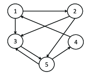
Figure 1: Small directed graph used for illustration of the ratio algorithm for obtaining average consensus in the presence of packet-dropping communication links.

III-A Examples

We now illustrate how the proposed algorithm works for the case of average consensus in the presence of packet-dropping communication links. We start with the rather small network shown in Fig. 1 and assume that the packets on each link (including the self-links which are not drawn in the figure) can be dropped with probability $1-q$, independently between different links and independently between different iterations. We also assume that the initial values of the five nodes are given by $v=[-4,5,6,-3,1]^{T}$, with their average equal to $1$. Thus, in the iterations (12) and (14)

$$y[0]=[-4,5,6,-3,1]^{T},\mbox{ and }z[0]=[1,1,1,1,1]^{T}\;,$$

with $\mu_{ji}[-1]=v_{ji}[-1]=\sigma_{ji}[-1]=\tau_{ji}[-1]=0$ for all $(j,i)\in\cal{E}$.

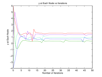
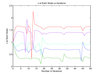
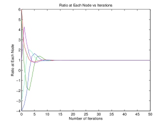
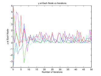
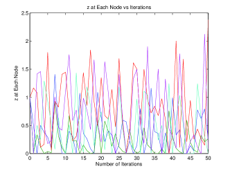
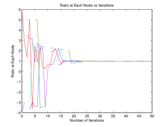
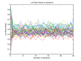
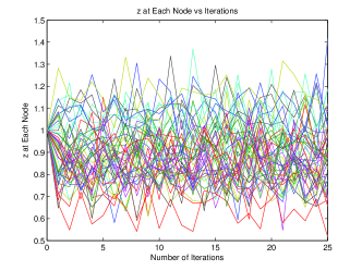
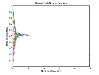
We run the iterations in (12) and (14) and plot the ratio $\frac{y_{j}[k]}{z_{j}[k]}$ as a function of the iteration step $k$ for each node $j$ ($j=1,2,3,4,5$). Figure 2 shows the typical behavior that we observe for $q=0.99$ (i.e., for a probability of a packet drop equal to $0.01$). As can be seen in the figure, the ratio at each node quickly converges to the correct average, though the individual values for $y_{j}[k]$ and $z_{j}[k]$ do not converge.

Figure 2: Evolution of the values of $y_{j}[k]$ (left), $z_{j}[k]$ (middle) and $\frac{y_{j}[k]}{z_{j}[k]}$ (right) for $q=0.99$.

Figure 3: Evolution of the values of $y_{j}[k]$ (left), $z_{j}[k]$ (middle), and $\frac{y_{j}[k]}{z_{j}[k]}$ (right) for $q=0.5$, $j=1,2,3,4,5$.

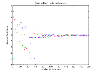
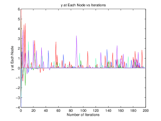
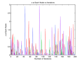
In Figs. 3 and 4 we show typical behaviors of the same multicomponent system for $q=0.5$ and $q=0.1$. The behavior remains similar to the one observed before: even though $y_{j}[k]$ and $z_{j}[k]$ do not converge (in fact, they seem to behave more radically with decreasing $q$), the ratio $\frac{y_{j}[k]}{z_{j}[k]}$ does converge to the average of the initial values. Note that the plot of the ratio in Fig. 4 is quite different than the rest: in this case, $q$ is small enough so that $z_{j}[k]$ (and simultaneously $y_{j}[k]$) can take the value zero (e.g., when all packets destined to node $j$ are dropped at iteration $k$); thus, the ratio in such cases is not defined and is not plotted, resulting in a discontinuous set of points in the plot. Nevertheless, we can see that when packets are received (which happens frequently enough for each node), the ratio has the correct value. This is a point addressed later in the paper.

Figure 4: Evolution of the values of $y_{j}[k]$ (left), $z_{j}[k]$ (middle), and $\frac{y_{j}[k]}{z_{j}[k]}$ (right) for $q=0.1$, $j=1,2,3,4,5$.

Figure 5: Evolution of the values of $y_{j}[k]$ (left), $z_{j}[k]$ (middle), and $\frac{y_{j}[k]}{z_{j}[k]}$ (right) for $q=0.1$ for a 50-component system.

An example of what happens in larger graphs is shown in Fig. 5. Here we consider a graph with $50$ nodes, randomly generated by choosing a directed edge from node $i$ to node $j$, $1\leq i,j\leq 50$, $i\neq j$, independently with probability $1/2$, and ensuring that the resulting graph is strongly connected. As can be seen the behavior remains similar to what we observed for the smaller graph: the ratio $\frac{y_{j}[k]}{z_{j}[k]}$ converges quickly to the average even though the individual $y_{j}[k]$ and $z_{j}[k]$ do not converge. For this particular plot, we used $q=0.1$, which also justifies the fluctuation in the values of $y_{j}[k]$ and $z_{j}[k]$.

IV First and Second Moment Analysis

In this section, we obtain recurrence relations that describe the first and second moment of the iterations after (12) and (14); this analysis is used in Section V to establish the claims in (16) and (17). In order to ease the moment calculations, the expressions in (12)–(14) will be rewritten more compactly in vector form. Also, in order to facilitate notation, we will allow each node $j$ to drop the packet carrying its own previous value when updating its value. This way, node $j$ handles its own value in the same way as its neighbors’ values and notation is simplified significantly.

IV-A Vectorized Description of Double-Iteration Algorithm

Using the definition for the indicator variable $x_{ji}[k]$ given in (3) and the resulting indicator variable $\ell_{ji}[k]$ given in (6), which describes the successful transmission of information from node $i$ to node $j$ over an existing, unreliable communication link, iterations (12) and (14) can be rewritten as

$$\mu_{lj}[k] =\left\{\begin{array}[]{cc}\mu_{lj}[k-1]+\frac{1}{\mathcal{D}_{j}^{+}}y_{j}[k],&\text{if }l\in\mathcal{N}_{j}^{+},\quad k\geq 0,\\ 0,&\text{if }l\notin\mathcal{N}_{j}^{+},\quad k\geq 0,\end{array}\right.$$ (20)

$$\nu_{ji}[k] =\left\{\begin{array}[]{cc}\mu_{ji}[k]x_{ji}[k]+\nu_{ji}[k-1](1-x_{ji}[k]),&\text{if }i\in\mathcal{N}_{j}^{-},\quad k\geq 0,\\ 0,&\text{if }i\notin\mathcal{N}_{j}^{-},\quad k\geq 0,\end{array}\right.$$ (23)

$$y_{j}[k+1] =\sum_{i=1}^{n}\big{(}\nu_{ji}[k]-\nu_{ji}[k-1]\big{)},\quad k\geq 0,$$ (24)

and

$$\sigma_{lj}[k] =\left\{\begin{array}[]{cc}\sigma_{lj}[k-1]+\frac{1}{\mathcal{D}_{j}^{+}}z_{j}[k],&\text{if }l\in\mathcal{N}_{j}^{+},\quad k\geq 0,\\ 0,&\text{if }l\notin\mathcal{N}_{j}^{+},\quad k\geq 0,\end{array}\right.$$ (27)

$$\tau_{ji}[k] =\left\{\begin{array}[]{cc}\sigma_{ji}[k]x_{ji}[k]+\tau_{ji}[k-1](1-x_{ji}[k]),&\text{if }i\in\mathcal{N}_{j}^{-},\quad k\geq 0,\\ 0,&\text{if }i\in\mathcal{N}_{j}^{-},\quad k\geq 0,\end{array}\right.$$ (30)

$$z_{j}[k+1] =\sum_{i=1}^{n}\big{(}\tau_{ji}[k]-\tau_{ji}[k-1]\big{)},\quad k\geq 0,$$ (31)

where $\mu_{lj}[-1]=\nu_{ji}[-1]=\sigma_{lj}[-1]=\tau_{ji}[-1]=0,~{}\forall j,i$.

Let $A\circ B$ denote the Hadamard (entry-wise) product of a pair of matrices $A$ and $B$ of identical size. Then, for all $k\geq 0$, iteration (20)–(24) can be rewritten in matrix form as

$$M_{k}=M_{k-1}+P\text{diag}(y_{k}),$$ (32)

$$N_{k}=M_{k}\circ X_{k}+N_{k-1}\circ(U-X_{k}),$$ (33)

$$y_{k+1}=(N_{k}-N_{k-1})e=\big{[}(M_{k}-N_{k-1})\circ X_{k}\big{]}e,$$ (34)

where $P=[p_{ji}]\in\mathbb{R}^{n\times n}$, with $p_{ji}=\frac{1}{\mathcal{D}_{i}^{+}},~{}\forall j\in\mathcal{N}_{i}^{+}$ and $p_{ji}=0$ otherwise; $M_{-1}=N_{-1}=0$; $y_{k}=y[k]$; $U\in\mathbb{R}^{n\times n}$, with $[U_{ji}]=1,~{}\forall i,j$; $\text{diag}(y_{k})$ is the diagonal matrix that results by having the entries of $y_{k}$ on the main diagonal; and $e=[1,1,\dots,1]^{\prime}$ (note that $U=ee^{T}$). Similarly, for $k\geq 0$, (27)–(31) can be rewritten in matrix form as

$$S_{k}=S_{k-1}+P\text{diag}(z_{k}),$$ (35)

$$T_{k}=S_{k}\circ X_{k}+T_{k-1}\circ(U-X_{k}),$$ (36)

$$z_{k+1}=(T_{k}-T_{k-1})e=\big{[}(S_{k}-T_{k-1})\circ X_{k}\big{]}e,$$ (37)

where $S_{-1}=T_{-1}=0$, $z_{k}=z[k]$, and $\text{diag}(z_{k})$ is the diagonal matrix that results by having the entries of $z_{k}$ on the main diagonal.

By defining $A_{k}:=M_{k}-N_{k-1}$ and $B_{k}:=S_{k}-T_{k-1}$, iteration (32)–(34) can be rewritten more compactly as

$$A_{k}=A_{k-1}\circ(U-X_{k-1})+P\text{diag}(y_{k}),\quad k\geq 1,$$ (38)

$$y_{k+1}=(A_{k}\circ X_{k})e,\quad k\geq 0,$$ (39)

and iteration (35)–(37) as

$$B_{k}=B_{k-1}\circ(U-X_{k-1})+P\text{diag}(z_{k}),\quad k\geq 1,$$ (40)

$$z_{k+1}=(B_{k}\circ X_{k})e,\quad k\geq 0,$$ (41)

where $A_{0}=M_{0}-N_{-1}=P\text{diag}(y_{0})$, and $B_{0}=S_{0}-T_{-1}=P\text{diag}(z_{0})$.

For analysis purposes, each matrix in (38)–(39) and (40)–(41) will be rewritten in vector form by stacking up the corresponding columns. Then, (38)–(39) and (40)–(41) can be rewritten in vector form as follows. Let $F=[I_{n}~{}I_{n}~{}\dots~{}I_{n}]\in\mathbb{R}^{n\times n^{2}}$, where $I_{n}$ is the $n\times n$ identity matrix, and $\tilde{P}=[E_{1}P^{T}~{}E_{2}P^{T}~{}\dots~{}E_{n}P^{T}]^{T}\in\mathbb{R}^{n^{2}\times n}$, where $E_{i}\in\mathbb{R}^{n\times n}$ has $E_{i}(i,i)=1$ and all other entries equal zero. [The entries of $E_{i}P^{T}\in\mathbb{R}^{n\times n}$ ($PE_{i}^{T}=PE_{i}$) are all zero except for the $i^{th}$ row (column) entries, which are those of the $i^{th}$ row (column) of matrix $P^{T}$ ($P$).] Then, (38)–(39) can be rewritten as

$$a_{k}=a_{k-1}\circ(u-x_{k-1})+\tilde{P}y_{k},\quad k\geq 1,$$ (42)

$$y_{k+1}=F(a_{k}\circ x_{k}),\quad k\geq 0,$$ (43)

where $a_{k}\in\mathbb{R}^{n^{2}}$, $x_{k}\in\mathbb{R}^{n^{2}}$, and $x_{k-1}\in\mathbb{R}^{n^{2}}$ result from stacking the columns of matrices $A_{k}$, $X_{k}$, and $X_{k-1}$, respectively. Similarly, (40)–(41) can be rewritten as

$$b_{k}=b_{k-1}\circ(u-x_{k-1})+\tilde{P}z_{k},\quad k\geq 1,$$ (44)

$$z_{k+1}=F(b_{k}\circ x_{k}),\quad k\geq 0,$$ (45)

where $b_{k}\in\mathbb{R}^{n^{2}}$ results from stacking the columns of matrix $B_{k}$.

Remark 1

It is important to note that matrices $A_{k}$ and $B_{k}$, and their corresponding vectors $a_{k}$ and $b_{k}$, have some entries that remain at zero for all $k\geq 0$. Specifically, the $(j,i)$ entry of matrices $A_{k}$ and $B_{k}$ (and their corresponding entries in $a_{k}$ and $b_{k}$) remain zero if there is no communication link from node $i$ to node $j$, i.e., $(j,i)\notin\mathcal{E}$. The reason we keep these entries (despite the fact they are zero and do not play a role in the analysis) is because they facilitate matrix notation and calculations in subsequent developments. ∎

Since it will appear later at several points of the analysis, it is worth noting that when premultiplying $\tilde{P}$ by $F$, we recover the matrix $P$, i.e.,

$$P=F\tilde{P}.$$ (46)

IV-B First Moment Analysis

In this section, we describe the first moment dynamics of (42)–(45) via discrete-time transition systems with no inputs, where (as shown below) the corresponding transition matrices (which are obtained from $P$ and $q$) are column stochastic and primitive. In both iterations, the sum of the entries of the first moment vectors for $y_{k}$ and $z_{k}$ is shown to remain constant over time and be respectively equal to the sum of $q\sum_{i}y_{0}(i)$ and $q\sum_{i}z_{0}(i)$. Furthermore, both first moments $\mathop{\bf E\/}[y_{k}]$ and $\mathop{\bf E\/}[z_{k}]$ are shown to reach a steady-state value as $k$ goes to infinity. The above discussion is formalized in the following lemma.

Lemma 1

Let $a_{k}$, $b_{k}$, $y_{k}$, and $z_{k}$ be described by the recurrence relations in (42)–(43), and (44)–(45) respectively. Let the first moments of $a_{k}$, $y_{k}$, $b_{k}$, and $z_{k}$ (i.e., $\mathop{\bf E\/}[a_{k}]$, $\mathop{\bf E\/}[y_{k}]$, $\mathop{\bf E\/}[b_{k}]$, and $\mathop{\bf E\/}[z_{k}]$) be denoted by $\overline{a}_{k}$, $\overline{y}_{k}$, $\overline{b}_{k}$, and $\overline{z}_{k}$ respectively. Then the evolution of $\overline{a}_{k}$, $\overline{y}_{k}$, $\overline{b}_{k}$, and $\overline{z}_{k}$, $\forall k\geq 1$, is governed by

$$\overline{a}_{k}=\big{[}q\tilde{P}F+(1-q)I_{n^{2}}\big{]}\overline{a}_{k-1},$$ (47)

$$\overline{y}_{k+1}=\big{[}qP+(1-q)I_{n}\big{]}\overline{y}_{k},$$ (48)

$$\overline{b}_{k}=\big{[}q\tilde{P}F+(1-q)I_{n^{2}}\big{]}\overline{b}_{k-1},$$ (49)

$$\overline{z}_{k+1}=\big{[}qP+(1-q)I_{n}\big{]}\overline{z}_{k},$$ (50)

where $I_{m}$ is the $m\times m$ identity matrix, with $\overline{a}_{0}=\tilde{P}y_{0}$, $\overline{y}_{1}=qPy_{0}$, $\overline{b}_{0}=\tilde{P}z_{0}$, and $\overline{z}_{1}=qPz_{0}$.

Proof:

Since the development for obtaining $\overline{a}_{k}$ and $\overline{y}_{k}$ is parallel to that for obtaining $\overline{b}_{k}$ and $\overline{z}_{k}$, our analysis focuses on the first case. For $k=0$ in (42)–(43), by taking expectations of both sides and noting that packet drops at time step $k=0$ are independent of the initial values for $a_{0}$, it follows that

$$\overline{a}_{0}=\tilde{P}y_{0},$$ (51)

$$\overline{y}_{1}=qF\overline{a}_{0}.$$ (52)

Substituting (51) into (52), we obtain $\overline{y}_{1}=qF\tilde{P}\overline{y}_{0}=qP\overline{y}_{0}$.

For $k\geq 1$ in (42)–(43), noting that packet drops at time step $k$ are independent of previous packet drops and the initial values of $a_{0}$, it follows, by taking expectations on both sides, that

$$\overline{a}_{k}=\overline{a_{k-1}\circ(u-x_{k-1})}+\overline{\tilde{P}y_{k}}=\overline{a}_{k-1}\circ(u-\overline{x}_{k-1})+\tilde{P}\overline{y}_{k}=(1-q)\overline{a}_{k-1}+\tilde{P}\overline{y}_{k},$$ (53)

$$\overline{y}_{k+1}=\overline{F(a_{k}\circ x_{k})}=F(\overline{a}_{k}\circ\overline{x}_{k})=qF\overline{a}_{k}.$$ (54)

Substituting (54) into (53), we obtain

$$\overline{a}_{k} =(1-q)\overline{a}_{k-1}+q\tilde{P}F\overline{a}_{k-1}$$ (55)

$$=[q\tilde{P}F+(1-q)I_{n^{2}}]\overline{a}_{k-1},$$ (56)

Similarly, substituting (53) into (54), we have

$$\overline{y}_{k+1} =(1-q)qF\overline{a}_{k-1}+qF\tilde{P}\overline{y}_{k}$$ (57)

$$=(1-q)\overline{y}_{k}+qF\tilde{P}\overline{y}_{k}$$ (58)

$$=[qP+(1-q)I_{n}]\overline{y}_{k},$$ (59)

where $I_{n}$ is the $n\times n$ identity matrix. ∎

IV-C Second Moment Analysis

In the order to calculate the second moment dynamics for (42)–(45), we utilize in the following lemma.

Lemma 2

Let $x$, $c$ and $d$ be random vectors of dimension $n$. Furthermore, assume that the entries of $x$ are Bernoulli i.i.d. random variables such that $\Pr\{x_{i}=1\}=q$ and $\Pr\{x_{i}=0\}=1-q$, $\forall i=1,2,\dots n$, and are independent from $c$ and $d$. Then

$$S:=\mathop{\bf E\/}\big{[}(c\circ x)(x\circ d)^{T}]=q^{2}\mathop{\bf E\/}[cd^{T}]+q(1-q)\mathop{\bf E\/}\big{[}\text{diag}(cd^{T})],$$ (60)

$$T:=\mathop{\bf E\/}\big{[}\big{(}c\circ x\big{)}\big{(}(u-x)\circ d\big{)}^{T}]=q(1-q)\mathop{\bf E\/}[cd^{T}]-q(1-q)\mathop{\bf E\/}\big{[}\text{diag}(cd^{T})],$$ (61)

where $\text{diag}(cd^{T})$ is a diagonal matrix with the same diagonal as matrix $cd^{T}$.

Proof:

The $(i,j),i\neq j$, entry of $S$ can be obtained as follows:

$$S_{ij}=\mathop{\bf E\/}\big{[}c_{i}x_{i}d_{j}x_{j}\big{]}.$$ (62)

Since $x_{i}$ and $x_{j}$ are pairwise independent, and independent from $c$ and $d$, it follows that

$$\mathop{\bf E\/}\big{[}c_{i}x_{i}d_{j}x_{j}\big{]}=q^{2}\mathop{\bf E\/}\big{[}c_{i}d_{j}\big{]}.$$ (63)

For $i=j$, observing that $\mathop{\bf E\/}[x_{i}x_{i}]=\mathop{\bf E\/}[x_{i}]=q,~{}\forall i=1,\dots,n$, we obtain the corresponding entry of $S$ as

$$S_{ii} =\mathop{\bf E\/}\big{[}c_{i}x_{i}d_{i}x_{i}\big{]}=\mathop{\bf E\/}\big{[}c_{i}d_{i}x_{i}\big{]}=q\mathop{\bf E\/}\big{[}c_{i}d_{i}\big{]}.$$ (64)

In (63), it is easy to see that $\mathop{\bf E\/}\big{[}c_{i}d_{j}\big{]}$ is the $(i,j)$ entry of $\mathop{\bf E\/}[cd^{T}]$. Similarly, in (64), it is easy to see that $\mathop{\bf E\/}\big{[}c_{i}d_{i}\big{]}$ is the $(i,i)$ entry of $\mathop{\bf E\/}[cd^{T}]$. From these observations, the result in (60) follows.

Similarly, the $(i,j),i\neq j$, entry of $T$ can be obtained as follows:

$$T_{ij}=\mathop{\bf E\/}\big{[}c_{i}x_{i}d_{j}(1-x_{j})\big{]}.$$ (65)

Since $x_{i}$ and $(1-x_{j})$ are independent, it follows that

$$\mathop{\bf E\/}\big{[}c_{i}x_{i}d_{j}(1-x_{j})\big{]}=\mathop{\bf E\/}\big{[}c_{i}d_{j}\big{]}\mathop{\bf E\/}\big{[}x_{i}(1-x_{j})\big{]}=q(1-q)\mathop{\bf E\/}\big{[}c_{i}d_{j}\big{]}.$$ (66)

For $i=j$, and observing that $\mathop{\bf E\/}[x_{i}(1-x_{i})]=0,~{}\forall i=1,\dots,n$, the corresponding entry of $T$ can obtained as follows;

$$T_{ii} =\mathop{\bf E\/}\big{[}c_{i}x_{i}d_{i}(1-x_{i})\big{]}=\mathop{\bf E\/}\big{[}c_{i}d_{i}\big{]}\mathop{\bf E\/}\big{[}x_{i}(1-x_{i})\big{]}=0.$$ (67)

The result in (61) follows from (66) and (67). ∎

The following lemma establishes that the evolution of $\mathop{\bf E\/}[a_{k}a_{k}^{T}]$, $\mathop{\bf E\/}[b_{k}b_{k}^{T}]$, and $\mathop{\bf E\/}[a_{k}b_{k}^{T}]$, and can be expressed as linear iterations with identical dynamics but different initial conditions. Similarly, the evolution of $\mathop{\bf E\/}[y_{k}y_{k}^{T}]$, $\mathop{\bf E\/}[z_{k}z_{k}^{T}]$, and $\mathop{\bf E\/}[y_{k}z_{k}^{T}]$ can also be expressed as linear iterations with identical dynamics but different initial conditions.

Lemma 3

Consider the second moments of $a_{k}$, $y_{k}$, $b_{k}$, and $z_{k}$, and let $\mathop{\bf E\/}[a_{k}a_{k}^{T}]$, $\mathop{\bf E\/}[y_{k}y_{k}^{T}]$, $\mathop{\bf E\/}[b_{k}b_{k}^{T}]$, $\mathop{\bf E\/}[z_{k}z_{k}^{T}]$, $\mathop{\bf E\/}[a_{k}b_{k}^{T}]$, and $\mathop{\bf E\/}[y_{k}z_{k}^{T}]$) be denoted by $\Gamma_{k}$, $\Phi_{k}$, $\Psi_{k}$, $\Lambda_{k}$, $\Xi_{k}$, and $\Upsilon_{k}$ respectively. Then, the evolutions of $\Gamma_{k}$, $\Phi_{k}$, $\Psi_{k}$, $\Lambda_{k}$, $\Xi_{k}$, $\Upsilon_{k},~{}\forall k\geq 1$, are described by the following iterations (where all $I$ denote $n^{2}\times n^{2}$ identity matrices):

$$\Gamma_{k} =\big{[}q\tilde{P}F+(1-q)I\big{]}\Gamma_{k-1}\big{[}q\tilde{P}F+(1-q)I\big{]}^{T}+q(1-q)[I-\tilde{P}F]\text{diag}(\Gamma_{k-1})[I-\tilde{P}F]^{T},$$ (68)

$$\Phi_{k+1} =F\big{[}q^{2}\Gamma_{k}+q(1-q)\text{diag}(\Gamma_{k})\big{]}F^{T},$$ (69)

$$\Psi_{k} =\big{[}q\tilde{P}F+(1-q)I\big{]}\Psi_{k-1}\big{[}q\tilde{P}F+(1-q)I\big{]}^{T}+q(1-q)[I-\tilde{P}F]\text{diag}(\Psi_{k-1})[I-\tilde{P}F]^{T},$$ (70)

$$\Lambda_{k+1} =F\big{[}q^{2}\Psi_{k}+q(1-q)\text{diag}(\Psi_{k})\big{]}F^{T},$$ (71)

$$\Xi_{k} =\big{[}q\tilde{P}F+(1-q)I\big{]}\Xi_{k-1}\big{[}q\tilde{P}F+(1-q)I\big{]}^{T}+q(1-q)[I-\tilde{P}F]\text{diag}(\Xi_{k-1})[I-\tilde{P}F]^{T},$$ (72)

$$\Upsilon_{k+1} =F\big{[}q^{2}\Xi_{k}+q(1-q)\text{diag}(\Xi_{k})\big{]}F^{T},$$ (73)

with initial conditions

$$\Gamma_{0}=\tilde{P}y_{0}y_{0}^{T}\tilde{P}^{T},$$ (74)

$$\Phi_{1}=\overline{y}_{1}\overline{y}_{1}^{T}+q(1-q)F\text{diag}(\tilde{P}y_{0}y_{0}^{T}\tilde{P}^{T})F^{T},$$ (75)

$$\Psi_{0}=\tilde{P}z_{0}z_{0}^{T}\tilde{P}^{T},$$ (76)

$$\Lambda_{1}=\overline{z}_{1}\overline{z}_{1}^{T}+q(1-q)F\text{diag}(\tilde{P}z_{0}z_{0}^{T}\tilde{P}^{T})F^{T},$$ (77)

$$\Xi_{0}=\tilde{P}y_{0}z_{0}^{T}\tilde{P}^{T},$$ (78)

$$\Upsilon_{1}=\overline{y}_{1}\overline{z}_{1}^{T}+q(1-q)F\text{diag}(\tilde{P}y_{0}z_{0}^{T}\tilde{P}^{T})F^{T}.$$ (79)

Proof:

The derivation of (68), (69), (74), and (75), is the same as the derivation of (70), (71), (76), and (77), thus the developments in the proof will only address the former. For $k=0$, it follows from Lemma 1 and (42) that $a_{0}=\tilde{P}y_{0}$. Then,

$$\Gamma_{0}=\mathop{\bf E\/}[a_{0}a_{0}^{T}]=\tilde{P}\mathop{\bf E\/}[y_{0}y_{0}^{T}]\tilde{P}^{T}=\tilde{P}y_{0}y_{0}^{T}\tilde{P}^{T},$$ (80)

and

$$\Phi_{1}=\mathop{\bf E\/}[y_{1}y_{1}^{T}]=\mathop{\bf E\/}\big{[}F(a_{0}\circ x_{0})(x_{0}\circ a_{0})^{T}F^{T}\big{]}=F\mathop{\bf E\/}\big{[}(a_{0}\circ x_{0})(x_{0}\circ a_{0})^{T}\big{]}F^{T}.$$ (81)

Applying the results in Lemmas 1 and 2 to (81), it follows that

$$\Phi_{1} =q^{2}F\mathop{\bf E\/}\big{[}a_{0}a_{0}^{T}\big{]}F^{T}+q(1-q)F\mathop{\bf E\/}\big{[}\text{diag}(a_{0}a_{0}^{T})\big{]}F^{T}$$

$$=(qF\tilde{P}y_{0})(qF\tilde{P}y_{0})^{T}+q(1-q)F\mathop{\bf E\/}[\text{diag}(\tilde{P}y_{0}y_{0}^{T}\tilde{P}^{T})]F^{T}$$

$$=(qPy_{0})(qPy_{0})^{T}+q(1-q)F\text{diag}(\tilde{P}y_{0}y_{0}^{T}\tilde{P}^{T})F^{T}$$

$$=\overline{y}_{1}\overline{y}_{1}^{T}+q(1-q)F\text{diag}(\tilde{P}y_{0}y_{0}^{T}\tilde{P}^{T})F^{T},$$ (82)

where we used the fact that $F\tilde{P}=P$ (refer to Eq. (46)).

For $k\geq 1$, and taking into account that $y_{k}=F(a_{k-1}\circ x_{k-1})$, it follows that

$$\Gamma_{k}= \mathop{\bf E\/}\big{[}\big{(}a_{k-1}\circ(u-x_{k-1})+\tilde{P}y_{k}\big{)}\big{(}a_{k-1}\circ(u-x_{k-1})+\tilde{P}y_{k}\big{)}^{T}\big{]}$$

$$= \mathop{\bf E\/}\big{[}\big{(}a_{k-1}\circ(u-x_{k-1})\big{)}\big{(}a_{k-1}\circ(u-x_{k-1})\big{)}^{T}\big{]}+\mathop{\bf E\/}\big{[}\big{(}a_{k-1}\circ(u-x_{k-1})\big{)}\big{(}\tilde{P}y_{k}\big{)}^{T}\big{]}$$

$$+\mathop{\bf E\/}\big{[}\big{(}\tilde{P}y_{k}\big{)}\big{(}a_{k-1}\circ(u-x_{k-1})\big{)}^{T}\big{]}+\mathop{\bf E\/}\big{[}\big{(}\tilde{P}y_{k}\big{)}\big{(}\tilde{P}y_{k}\big{)}^{T}\big{]}$$

$$= \mathop{\bf E\/}\big{[}\big{(}a_{k-1}\circ(u-x_{k-1})\big{)}\big{(}a_{k-1}\circ(u-x_{k-1})\big{)}^{T}\big{]}+\mathop{\bf E\/}\big{[}\big{(}a_{k-1}\circ(u-x_{k-1})\big{)}\big{(}a_{k-1}\circ x_{k-1}\big{)}^{T}\big{]}F^{T}\tilde{P}^{T}$$

$$+\tilde{P}F\mathop{\bf E\/}\big{[}\big{(}a_{k-1}\circ x_{k-1}\big{)}\big{(}a_{k-1}\circ(u-x_{k-1})\big{)}^{T}\big{]}+\tilde{P}F\mathop{\bf E\/}\big{[}\big{(}a_{k-1}\circ x_{k-1}\big{)}\big{(}a_{k-1}\circ x_{k-1}\big{)}^{T}\big{]}F^{T}\tilde{P}^{T}.$$ (83)

Then, from Lemma 2, (83) can be rewritten as

$$\Gamma_{k}= (1-q)^{2}\mathop{\bf E\/}\big{[}a_{k-1}a_{k-1}^{T}\big{]}+q(1-q)\mathop{\bf E\/}\big{[}\text{diag}(a_{k-1}a_{k-1}^{T})]$$

$$+q(1-q)\mathop{\bf E\/}\big{[}a_{k-1}a_{k-1}^{T}\big{]}F^{T}\tilde{P}^{T}-q(1-q)\mathop{\bf E\/}\big{[}\text{diag}(a_{k-1}a_{k-1}^{T})]F^{T}\tilde{P}^{T}$$

$$+q(1-q)\tilde{P}F\mathop{\bf E\/}\big{[}a_{k-1}a_{k-1}^{T}\big{]}-q(1-q)\tilde{P}F\mathop{\bf E\/}\big{[}\text{diag}(a_{k-1}a_{k-1}^{T})]$$

$$+q^{2}\tilde{P}F\mathop{\bf E\/}\big{[}a_{k-1}a_{k-1}^{T}\big{]}F^{T}\tilde{P}^{T}+q(1-q)\tilde{P}F\mathop{\bf E\/}\big{[}\text{diag}(a_{k-1}a_{k-1}^{T})]F^{T}\tilde{P}^{T}.$$ (84)

By re-arranging terms in (84) and observing that $\Gamma_{k-1}=\mathop{\bf E\/}\big{[}a_{k-1}a_{k-1}^{T}\big{]}$ and $\text{diag}(\Gamma_{k-1})=\mathop{\bf E\/}\big{[}\text{diag}(a_{k-1}a_{k-1}^{T})\big{]}$, the result in (68) follows.

Additionally, from Lemma 2, it follows that

$$\Phi_{k+1}=\mathop{\bf E\/}\big{[}y_{k+1}y_{k+1}^{T}\big{]} =F\mathop{\bf E\/}\big{[}(a_{k}\circ x_{k})(x_{k}\circ a_{k})^{T}\big{]}F^{T}$$

$$=F\Big{[}q^{2}\mathop{\bf E\/}\big{[}a_{k}a_{k}^{T}\big{]}+q(1-q)\mathop{\bf E\/}\big{[}\text{diag}(a_{k}a_{k}^{T})\big{]}\Big{]}F^{T}$$

$$=F\big{[}q^{2}\Gamma_{k}+q(1-q)\text{diag}(\Gamma_{k})\big{]}F^{T}.$$ (85)

To obtain the iterations for $\Xi_{k}$ and $\Upsilon_{k}$, the developments are very similar to the ones above. For $k=0$,

$$\Xi_{0}=\mathop{\bf E\/}\big{[}a_{0}b_{0}^{T}\big{]}=\tilde{P}\mathop{\bf E\/}[y_{0}z_{0}^{T}]\tilde{P}^{T}=\tilde{P}y_{0}z_{0}^{T}\tilde{P},$$ (86)

and

$$\Upsilon_{1}=\mathop{\bf E\/}[y_{1}z_{1}^{T}] =\mathop{\bf E\/}\big{[}F(a_{0}\circ x_{0})(x_{0}\circ b_{0})^{T}F^{T}\big{]}=F\mathop{\bf E\/}\big{[}(a_{0}\circ x_{0})(x_{0}\circ b_{0})^{T}\big{]}F^{T}$$

$$=(qF\tilde{P}y_{0})(qF\tilde{P}z_{0})^{T}+q(1-q)F\mathop{\bf E\/}[\text{diag}(\tilde{P}y_{0}z_{0}^{T}\tilde{P}^{T})]F^{T}$$

$$=(qPy_{0})(qPz_{0})^{T}+q(1-q)F\text{diag}(\tilde{P}y_{0}z_{0}^{T}\tilde{P}^{T})F^{T}$$

$$=\overline{y}_{1}\overline{z}_{1}^{T}+q(1-q)F\text{diag}(\tilde{P}y_{0}z_{0}^{T}\tilde{P}^{T})F^{T},$$ (87)

where again we used the fact that $F\tilde{P}=P$ (refer to Eq. (46)).

For $k\geq 1$, from Lemma 2 and (42), and taking into account that $y_{k+1}=F(a_{k}\circ x_{k})$ and $z_{k+1}=F(b_{k}\circ x_{k})$, it follows that

$$\Xi_{k}= \mathop{\bf E\/}\big{[}\big{(}a_{k-1}\circ(u-x_{k-1})+\tilde{P}y_{k}\big{)}\big{(}b_{k-1}\circ(u-x_{k-1})+\tilde{P}z_{k}\big{)}^{T}\big{]}$$

$$= \mathop{\bf E\/}\big{[}\big{(}a_{k-1}\circ(u-x_{k-1})\big{)}\big{(}b_{k-1}\circ(u-x_{k-1})\big{)}^{T}\big{]}+\mathop{\bf E\/}\big{[}\big{(}a_{k-1}\circ(u-x_{k-1})\big{)}\big{(}\tilde{P}z_{k}\big{)}^{T}\big{]}$$

$$+\mathop{\bf E\/}\big{[}\big{(}\tilde{P}y_{k}\big{)}\big{(}b_{k-1}\circ(u-x_{k-1})\big{)}^{T}\big{]}+\mathop{\bf E\/}\big{[}\big{(}\tilde{P}y_{k}\big{)}\big{(}\tilde{P}z_{k}\big{)}^{T}\big{]}$$

$$= \mathop{\bf E\/}\big{[}\big{(}a_{k-1}\circ(u-x_{k-1})\big{)}\big{(}b_{k-1}\circ(u-x_{k-1})\big{)}^{T}\big{]}+\mathop{\bf E\/}\big{[}\big{(}a_{k-1}\circ(u-x_{k-1})\big{)}\big{(}b_{k-1}\circ x_{k-1}\big{)}^{T}\big{]}F^{T}\tilde{P}^{T}$$

$$+\tilde{P}F\mathop{\bf E\/}\big{[}\big{(}a_{k-1}\circ x_{k-1}\big{)}\big{(}b_{k-1}\circ(u-x_{k-1})\big{)}^{T}\big{]}+\tilde{P}F\mathop{\bf E\/}\big{[}\big{(}a_{k-1}\circ x_{k-1}\big{)}\big{(}b_{k-1}\circ x_{k-1}\big{)}^{T}\big{]}F^{T}\tilde{P}^{T}$$

$$= (1-q)^{2}\mathop{\bf E\/}\big{[}a_{k-1}b_{k-1}^{T}\big{]}+q(1-q)\mathop{\bf E\/}\big{[}\text{diag}(a_{k-1}b_{k-1}^{T})]$$

$$+q(1-q)\mathop{\bf E\/}\big{[}a_{k-1}b_{k-1}^{T}\big{]}F^{T}\tilde{P}^{T}-q(1-q)\mathop{\bf E\/}\big{[}\text{diag}(a_{k-1}b_{k-1}^{T})]F^{T}\tilde{P}^{T}$$

$$+q(1-q)\tilde{P}F\mathop{\bf E\/}\big{[}a_{k-1}b_{k-1}^{T}\big{]}-q(1-q)\tilde{P}F\mathop{\bf E\/}\big{[}\text{diag}(a_{k-1}b_{k-1}^{T})]$$

$$+q^{2}\tilde{P}F\mathop{\bf E\/}\big{[}a_{k-1}b_{k-1}^{T}\big{]}F^{T}\tilde{P}^{T}+q(1-q)\tilde{P}F\mathop{\bf E\/}\big{[}\text{diag}(a_{k-1}b_{k-1}^{T})]F^{T}\tilde{P}^{T}.$$ (88)

By re-arranging terms in (88) and observing that $\Xi_{k-1}=\mathop{\bf E\/}\big{[}a_{k-1}b_{k-1}^{T}\big{]}$ and $\text{diag}(\Xi_{k-1})=\mathop{\bf E\/}\big{[}\text{diag}(a_{k-1}b_{k-1}^{T})\big{]}$, the result in (72) follows. Finally,

$$\Upsilon_{k+1}=\mathop{\bf E\/}\big{[}y_{k+1}z_{k+1}^{T}\big{]} =F\mathop{\bf E\/}\big{[}(a_{k}\circ x_{k})(x_{k}\circ b_{k})^{T}\big{]}F^{T}$$

$$=F\Big{[}q^{2}\mathop{\bf E\/}\big{[}a_{k}b_{k}^{T}\big{]}+q(1-q)\mathop{\bf E\/}\big{[}\text{diag}(a_{k}b_{k}^{T})\big{]}\Big{]}F^{T}$$

$$=F\big{[}q^{2}\Xi_{k}+q(1-q)\text{diag}(\Xi_{k})\big{]}F^{T},$$ (89)

which completes the proof. ∎

Although omitted in the statement of Lemma 3, it is easy to see that the dynamics of $\Delta_{k}=\mathop{\bf E\/}[b_{k}a_{k}^{T}]$ and $\Theta_{k}=\mathop{\bf E\/}[z_{k}y_{k}^{T}]$ can also be obtained by noting that $\Delta_{k}=\Psi_{k}^{T}$ and $\Theta_{k}=\Upsilon_{k}^{T}$.

V Convergence Analysis of Robustified Double-Iteration Algorithm

The previous Section established that the iterations governing the evolution of $\Gamma_{k}$, $\Psi_{k}$ and $\Xi_{k}$ are identical except for the initial conditions. We will show next that the steady-state solutions of these iterations are also identical up to a multiplicative constant. To see this, we will rewrite (68), (70), and (72) in vector form using Kronecker products. For given matrices $C$, $A$, and $B$ of appropriate dimensions, the matrix equation $C=AXB$ (where $X$ is an unknown matrix) can be rewritten as a set of linear equations of the form $(B^{T}\otimes A)x=c$, where $x$ and $c$ are the vectors that result from stacking the columns of matrices $X$ and $C$ respectively, and $\otimes$ denotes the Kronecker product of matrices [26]. Let $\gamma_{k}$ be the vector that results from stacking the columns of $\Gamma_{k}$ and $\tilde{\gamma}_{k}$ the vector that results from stacking the columns of $\text{diag}(\Gamma_{k})$. Then, it can be easily seen that (68) can be rewritten as

$$\gamma_{k}= \big{[}[q\tilde{P}F+(1-q)I]\otimes[q\tilde{P}F+(1-q)I]\big{]}\gamma_{k-1}+\big{[}q(1-q)[I-\tilde{P}F]\otimes[I-\tilde{P}F]\big{]}\tilde{\gamma}_{k-1},~{}k\geq 1.$$ (90)

Let $G$ be a diagonal matrix with entries $G\big{(}(l-1)n^{2}+l,(l-1)n^{2}+l\big{)}=1,~{}\forall l=1,2,\dots,n^{2}$, and zero otherwise. Then, the second term on the right hand side of (90) can be written as

$$q(1-q)\big{(}[I-\tilde{P}F]\otimes[I-\tilde{P}F]\big{)}\tilde{\gamma}_{k-1}=q(1-q)\big{(}[I-\tilde{P}F]\otimes[I-\tilde{P}F]\big{)}G\gamma_{k-1},~{}k\geq 1,$$ (91)

which leads us to

$$\gamma_{k}=\big{[}[q\tilde{P}F+(1-q)I]\otimes[q\tilde{P}F+(1-q)I]+q(1-q)\big{(}[I-\tilde{P}F]\otimes[I-\tilde{P}F]\big{)}G\big{]}\gamma_{k-1},~{}k\geq 1.$$ (92)

Let $\psi_{k}$ and $\xi_{k}$ and $\delta_{k}$ be the vectors that result from stacking the columns of $\Psi_{k}$, $\Xi_{k}$ and $\Delta_{k}$ respectively. Then, it is easy to see that the same recurrence relation as in (92) governs the evolution of $\psi_{k}$ and $\xi_{k}$.

Theorem 1

Let $P\in\mathbb{R}^{n\times n}$ be a column stochastic and primitive weight matrix associated with a directed graph $\mathcal{G}=\{\mathcal{V},\mathcal{E}\}$, with $\mathcal{V}=\{1,2,\dots,n\}$ and $\mathcal{E}\subseteq\mathcal{V}\times\mathcal{V}$. Let $F=[I_{n}~{}I_{n}~{}\dots~{}I_{n}]\in\mathbb{R}^{n\times n^{2}}$, where $I_{n}$ is the $n\times n$ identity matrix, and $\tilde{P}=[E_{1}P^{T}~{}E_{2}P^{T}~{}\dots~{}E_{n}P^{T}]^{T}\in\mathbb{R}^{n^{2}\times n}$, where each $E_{i}\in\mathbb{R}^{n\times n},~{}i\in\{1,2,\dots,n\}$, satisfies $E_{i}(i,i)=1$ and has all other entries equal to zero. Then, for any $q$, $0<q\leq 1$, the matrix $\Pi$ defined as

$$\Pi\equiv[q\tilde{P}F+(1-q)I]\otimes[q\tilde{P}F+(1-q)I]+q(1-q)\big{(}[I-\tilde{P}F]\otimes[I-\tilde{P}F]\big{)}G$$ (93)

is column stochastic, and it has a single eigenvalue of maximum magnitude at value one.

Proof:

We show first column stochasticity of matrix $\Pi$. Let $C=q\tilde{P}F+(1-q)I$ and $D=I-\tilde{P}F$, so that $\Pi=C\otimes C+q(1-q)(D\otimes D)G$. We will establish that $C\otimes C$ is column stochastic and also show that the column sums of $D\otimes D$ are all zero. By construction, the entries of the $i^{th}$ column of $\tilde{P}\in\mathbb{R}^{n^{2}\times n}$ are all zero, with the possible exception of the ones indexed by $\big{(}(i-1)n+j,i\big{)},~{}i,j=1,2,\dots,n$, each of which corresponds to the $(j,i)$ entry of matrix $P$. Then, it follows that $\sum_{l=1}^{n^{2}}\tilde{P}_{li}=\sum_{j=1}^{n}P_{ji}=1,\forall i=1,2,\dots,n^{2}$. The matrix $\tilde{P}F\in\mathbb{R}^{n^{2}\times n^{2}}$ is also column stochastic by construction, as it results from horizontally concatenating $n$ times the matrix $\tilde{P}$, i.e., $\tilde{P}F=[\tilde{P}~{}\tilde{P}~{}\dots~{}\tilde{P}]$; therefore, the matrix $C$ is also column stochastic. The kronecker product of $C$ with itself, results in an $n^{4}\times n^{4}$ block matrix of the form $C\otimes C=[C_{1}~{}C_{2}\dots~{}C_{n^{2}}]$, where $C_{j}=[c_{1j}C^{T}~{}c_{2j}C^{T}~{}\dots~{}c_{n^{2}j}C^{T}]^{T}$. Then, it follows that the sum of the entries of the $l^{th}$ column of $C_{j}$ is $\sum_{m=1}^{n^{4}}C_{j}(m,l)=(\sum_{i=1}^{n^{2}}c_{ij})(\sum_{r=1}^{n^{2}}c_{rl})$. Since $\sum_{i=1}^{n^{2}}c_{ij}$ and $\sum_{r=1}^{n^{2}}c_{rl}$ are the sum of the entries of the $j^{th}$ and $l^{th}$ columns of $C=q\tilde{P}F+(1-q)I_{n^{4}}$ (which is column stochastic), it follows that $\sum_{m=1}^{n^{4}}C_{j}(m,l)=1$; therefore, $C\otimes C$ is also column stochastic.

Since $\tilde{P}F$ is column stochastic, the column-sums of $D=I-\tilde{P}F$ are zero. The kronecker product of D with itself is of the form $D\otimes D=[D_{1}~{}D_{2}\dots~{}D_{n^{2}}]$, where $D_{j}=[d_{1j}D^{T}~{}d_{2j}D^{T}~{}\dots~{}d_{n^{2}j}D^{T}]^{T}$. Using similar arguments as above, it follows that $\sum_{m=1}^{n^{4}}D_{j}(m,l)=(\sum_{i=1}^{n^{2}}d_{ij})(\sum_{r=1}^{n^{2}}d_{rl})=0$, which implies that the column-sums of $D\otimes D$ are zero. The only thing left to establish that $\Pi$ is column stochastic is to show that all entries of $\Pi$ are nonnegative (from where it immediately follows that $\Pi=C\otimes C+q(1-q)(D\otimes D)G$ is column stochastic). We argue nonnegativity of $\Pi$ as follows: due to the sparsity structure of $G$ in (93), the only nonzero entries of $(D\otimes D)G$ will be in columns $(k-1)n^{2}+k,~{}k=1,2,\dots,n^{2}$; thus except for entries in these columns, the entries of $\Pi$ will be identical to the corresponding entries in $C\otimes C$. From the structure of $\tilde{P}F$, entries of $C\otimes C$ and $q(1-q)(D\otimes D)$ can, respectively, take one of the following three forms:

$$\big{(}qp_{ij}+(1-q)\big{)}\big{(}qp_{lm}+(1-q)\big{)},$$ (94)

$$q(1-q)(1-p_{ij})(1-p_{lm}),$$ (95)

or

$$qp_{ij}\big{(}qp_{lm}+(1-q)\big{)},$$ (96)

$$-q(1-q)p_{ij}(1-p_{lm}),$$ (97)

or

$$q^{2}p_{ij}p_{lm},$$ (98)

$$q(1-q)p_{ij}p_{lm},$$ (99)

where $p_{ij}\geq 0$ and $p_{lm}\geq 0$ are the $(i,j)$ and $(l,m)$ entries of matrix $P$. For (94) and (95), the corresponding entry of $\Pi$ is of the form

$$\big{(}qp_{ij}+(1-q)\big{)}\big{(}qp_{lm}+(1-q)\big{)}+q(1-q)(1-p_{ij})(1-p_{lm})=qp_{ij}p_{lm}+(1-q),$$ (100)

and satisfies $0\leq qp_{ij}p_{lm}+(1-q)\leq 1$ For (96) and (97), the corresponding entry of $\Pi$ is of the form

$$qp_{ij}\big{(}qp_{lm}+(1-q)\big{)}-q(1-q)p_{ij}(1-p_{lm})=qp_{ij}p_{lm},$$ (101)

and satisfies $0\leq qp_{ij}p_{lm}\leq 1$. For (98) and (99), the corresponding entry of $\Pi$ is of the form

$$q^{2}p_{ij}p_{lm}+q(1-q)p_{ij}p_{lm}=qp_{ij}p_{lm},$$ (102)

and satisfies $0\leq qp_{ij}p_{lm}\leq 1$.

To prove the second assertion, we will show first that matrix $\tilde{P}F$ can be written via a permutation of its indices in the form

$$\begin{bmatrix}U&&V\\ 0&&W\end{bmatrix},$$ (103)

where $U$ is an irreducible column stochastic matrix and $\lim_{k\rightarrow\infty}W^{k}=0$. Since $\tilde{P}F$ is column stochastic, we can assume that it corresponds to the weight matrix of some graph $\tilde{\mathcal{G}}=\{\tilde{\mathcal{V}},\tilde{\mathcal{E}}\}$. We will show that this graph has a single recurrent class plus a few transient states, from which the decomposition of $\tilde{P}F$ in (103) follows. Let

$$\tilde{\mathcal{V}}=\{(1,1),(2,1),\dots,(n,1),(1,2),(2,2),\dots,(n,2),\dots,(n,n-1),(1,n),(2,n),\dots,(n,n)\}.$$ (104)

From the structure of $\tilde{P}F$, it follows that for any node $(i,j)\in\tilde{\mathcal{V}}$, one-step transitions out of $(i,j)$ are to nodes of the form $(m,i)$, with $i\in\mathcal{N}_{m}^{-}$, where $\mathcal{N}_{m}^{-}$ is the set in-neighbors of node $m$ in the graph $\mathcal{G}$ (with weight matrix $P$). From the structure of $\tilde{P}F$, it also follows that there are possibly several rows of $\tilde{P}F$ with all entries equal to zero, which means that a node $(i,j)$ that is associated with such row cannot be reached from any other node; however, as already argued, from nodes of the form $(i,j)$, it is possible to reach nodes of the form $(m,i)$, where $i\in\mathcal{N}_{m}^{-}$. Clearly, the nodes corresponding to rows with all entries being zero are transient. Note that the possibility of individual nodes that cannot be reached from any other node being disconnected is ruled out as it is easy to see the only nonzero diagonal entries of $\tilde{P}F$ correspond to diagonal entries of $P$, which are strictly smaller than one.

Next we will show that from a node $(i,j)$ whose corresponding row in $\tilde{P}F$ has some nonzero entries one can reach any other node $(m,l)$ whose corresponding row in $\tilde{P}F$ has some nonzero entries. This means that all non-transient nodes form a single recurrent class (as already argued all nonzero diagonal entries are strictly smaller than one which means there cannot be absorbing nodes). This follows from the fact that the graph $\mathcal{G}$ is strongly connected, which means that for any $j,l\in\mathcal{V}$, there exists a path between $j$ and $l$. Let $i_{1},i_{2},\dots,i_{t}$ denote the nodes traversed along the path between $j$ and $l$. We will show next that for any two non-transient nodes $(i,j),(r,l)\in\tilde{\mathcal{V}}$ there exists a path. As already argued, from $(i,j)$ one can reach in a single hop any node of the form $(m,i)$, where $m$ is a neighbor of node $i$ in the graph $\mathcal{G}$. Since $i_{1}$ is the first node traversed in the path between $j$ and $l$, it follows that $(i_{1},i)\in\tilde{\mathcal{V}}$ can be reached in one step from $(i,j)$. By repeatedly using this argument, it follows that the sequence of nodes $(i_{1},i),(i_{2},i_{1}),\dots,(i_{t},i_{t-1}),(r,i_{t})$ forms a path between $(i,j)$ and $(r,l)$, which means that any non-transient node can be reached by any other non-transient node; thus, the set of non-transient nodes forms a single recurrent class. Clearly, the vertex set $\tilde{\mathcal{V}}$ can be decomposed into a single recurrent class and possibly several transient nodes. By re-ordering the nodes, it follows that $\tilde{P}F$ can be rewritten as in (103) (see, e.g., [27, p. 126]). Furthermore, since $Q$ in (103) is irreducible, it follows that $qQ+(1-q)I$ (where $I$ is the identity matrix) is primitive. It follows that $C=q\tilde{P}F+(1-q)I$ has a unique largest eigenvalue of value one, i.e., $\lambda_{1}=1$, and $1>|\lambda_{2}|\geq\dots\geq|\lambda_{n^{2}}|$. Let $\sigma(C)=\{\lambda_{1},\lambda_{2},\dots,\lambda_{n^{2}}\}$. Then, $\sigma(C\otimes C)=\{\lambda_{i}\lambda_{j},~{}i=1,\dots,n,~{}j=1,\dots,n\}$, including algebraic multiplicities in both cases [26, p. 245]. Since $\lambda_{1}=1$ is unique (multiplicity one) and $|\lambda_{i}|<1,~{}i=2,\dots,n^{2}$, it follows that the eigenvalue of $C\otimes C=[q\tilde{P}F+(1-q)I]\otimes[q\tilde{P}F+(1-q)I]$ of largest magnitude also takes value 1 and is unique. Since $C\otimes C$ is column stochastic and $\lambda_{1}=1$ is unique, we know that either $C\otimes C$ is also primitive or it can be decomposed following a permutation of indices to the form [27, p. 126]:

$$\begin{bmatrix}L&&M\\ 0&&N\end{bmatrix},$$ (105)

where $L$ is a primitive matrix and $\lim_{k\rightarrow\infty}N^{k}=0$.

We will show next that $\Pi=C\otimes C+q(1-q)(D\otimes D)G$ has exactly the same nonzero entries as $C\otimes C$ and therefore can be decomposed following the same permutation of indices to the form in (105). As argued before, due to the sparsity structure of $G$ in (93), the only nonzero entries of $(D\otimes D)G$ will be in columns $(k-1)n^{2}+k,~{}k=1,2,\dots,n^{2}$, thus except for entries in the aforementioned columns, the nonzero entries of $\Pi$ will be the same as those in $C\otimes C$. For all other columns in $\Pi$ (that include nonzero entries in $(D\otimes D)G$), it was shown in (100)–(102) that the nonzero entries of $\Pi$ are strictly positive, from where it follows that $\Pi$ has the same sparsity structure as $C\otimes C$, which means that $\Pi$ can also be decomposed in the form of (105) (for some matrices $L^{\prime}$, $M^{\prime}$, $N^{\prime}$), and the resulting upper-right block is also a primitive matrix. Therefore, $\Pi$ has a unique largest eigenvalue at one. ∎

The following two lemmas establish that the first and second moments of $a_{k}$ and $b_{k}$, and $y_{k}$ and $z_{k}$ converge to the same solution up to a scalar multiplication. These two lemmas will be used to show that as $k\rightarrow\infty$, the random vector $v_{k}=z_{k}-\alpha y_{k}$, for $\displaystyle\alpha=\frac{\sum_{j=1}^{n}z_{0}(j)}{\sum_{j=1}^{n}y_{0}(j)}$, will converge almost surely to $v=0$. This suggests that, as $k\rightarrow\infty$, and whenever $z_{k}$ is nonzero, each node $i$ can obtain an estimate of $\alpha=\frac{\sum_{j=1}^{n}z_{0}(j)}{\sum_{j=1}^{n}y_{0}(j)}$ by calculating the ratio $y_{k}(i)/z_{k}(i)$. We will also show that, in fact, $z_{k}$ will be larger than some threshold infinitely often.

Lemma 4

The first moments of $a_{k}$ and $b_{k}$ (also $y_{k}$ and $z_{k}$ asymptotically converge to the same solution up to scalar multiplication:

$$\lim_{k\rightarrow\infty}\overline{z}_{k}=\alpha\lim_{k\rightarrow\infty}\overline{y}_{k},$$ (106)

$$\lim_{k\rightarrow\infty}\overline{b}_{k}=\alpha\lim_{k\rightarrow\infty}\overline{a}_{k},$$ (107)

where $\displaystyle\alpha=\frac{\sum_{j=1}^{n}z_{0}(j)}{\sum_{j=1}^{n}y_{0}(j)}$.

Proof:

In Lemma 1, it was shown that $\overline{y}_{k+1}=\big{[}qP+(1-q)I\big{]}\overline{y}_{k}$ and $\overline{z}_{k+1}=\big{[}qP+(1-q)I\big{]}\overline{z}_{k}$ with $\overline{y}_{1}=qy_{0}$, and $\overline{z}_{1}=qz_{0}$. Since $P$ is column stochastic and primitive, it follows that $[qP+(1-q)I\big{]}$ is also column stochastic and primitive. Thus, $\lim_{k\rightarrow\infty}\overline{z}_{k}=\alpha\lim_{k\rightarrow\infty}\overline{y}_{k},$ where from the column stochasticity property it follows that $\sum_{j=1}^{n}\overline{z}_{k}(j)=q(\sum_{j=1}^{n}z_{0}(j))$ and $\sum_{j=1}^{n}\overline{y}_{k}(j)=q\big{(}\sum_{j=1}^{n}y_{0}(j)\big{)},~{}\forall k\geq 1$; this implies that $\alpha=\frac{\sum_{j=1}^{n}z_{0}(j)}{\sum_{j=1}^{n}y_{0}(j)}$, which establishes (106).

By noting that $\overline{a}_{0}=\tilde{P}y_{0}$, and $\overline{b}_{0}=\tilde{P}y_{0}$, and using the fact that $\tilde{P}$ is column stochastic, it follows that $\sum_{j=1}^{n}\overline{a}_{k}(j)=\sum_{j=1}^{n}\overline{a}_{0}(j)=\sum_{j=1}^{n}y_{0}(j)$ and $\sum_{j=1}^{n}\overline{b}_{k}(j)=\sum_{j=1}^{n}\overline{b}_{0}(j)=\sum_{j=1}^{n}z_{0}(j)$. Since $q\tilde{P}F+(1-q)I$ (i.e., the matrix that governs the dynamics of $\overline{a}_{k}$ and $\overline{b}_{k}$) is column stochastic and, as shown in the proof of Theorem 1, has a single largest eigenvalue at value 1, a similar development to the one above can be used to show (107). ∎

Lemma 5

Define $w_{k}=b_{k}-\alpha a_{k}$ and denote by $\chi_{k}$ the vector that results from stacking the columns of $X_{k}:=\mathop{\bf E\/}[w_{k}w_{k}^{T}]$. Then, it follows that

$$\chi_{k}=\Pi\chi_{k-1},$$ (108)

with $\chi_{0}=\psi_{0}+\alpha^{2}\gamma_{0}-\alpha(\xi_{0}+\delta_{0})$ and $\sum_{l=1}^{n^{4}}\chi_{0}(l)=0$.

Proof:

Since $X_{k}:=\mathop{\bf E\/}[w_{k}w_{k}^{T}]=\mathop{\bf E\/}[b_{k}b_{k}^{T}]+\alpha^{2}\mathop{\bf E\/}[a_{k}a_{k}^{T}]-\alpha(\mathop{\bf E\/}[a_{k}b_{k}^{T}]+\mathop{\bf E\/}[b_{k}a_{k}^{T}])=\Psi_{k}+\alpha^{2}\Gamma_{k}-\alpha(\Xi_{k}+\Delta_{k})$, it follows that $\chi_{k}=\psi_{k}+\alpha^{2}\gamma_{k}-\alpha(\xi_{k}+\delta_{k})$. From (92) and subsequent discussion, it follows that $\gamma_{k}=\Pi\gamma_{k-1}$, $\psi_{k}=\Pi\psi_{k-1}$, $\xi_{k}=\Pi\xi_{k-1}$, and $\delta_{k}=\Pi\delta_{k-1}$, thus $\chi_{k}=\Pi\psi_{k-1}+\alpha^{2}\Pi\gamma_{k-1}-\alpha(\Pi\xi_{k-1}+\Pi\delta_{k-1})=\Pi(\psi_{k-1}+\alpha^{2}\gamma_{k-1}-\alpha(\xi_{k-1}+\delta_{k-1}))=\Pi\chi_{k-1}$.

In Lemma 3, it was shown that $\Gamma_{0}=\tilde{P}y_{0}y_{0}^{T}\tilde{P}^{T}$, $\Psi_{0}=\tilde{P}z_{0}z_{0}^{T}\tilde{P}^{T}$, and $\Xi_{0}=\tilde{P}y_{0}z_{0}^{T}\tilde{P}^{T}=\Delta_{0}^{T}$. Since $\gamma_{0}$, $\psi_{0}$, $\xi_{0}$, and $\delta_{0}$ result from stacking the columns of $\Gamma_{0}$, $\Psi_{0}$, $\Xi_{0}$, and $\Delta_{0}$, it follows that

$$\sum_{l=1}^{n^{4}}\gamma_{0}(l)=\sum_{i=1}^{n^{2}}\sum_{j=1}^{n^{2}}\Gamma_{0}(i,j)=\left(\sum_{i=1}^{n}y_{0}(i)\right)^{2},$$ (109)

$$\sum_{l=1}^{n^{4}}\psi_{0}(l)=\sum_{i=1}^{n^{2}}\sum_{j=1}^{n^{2}}\Psi_{0}(i,j)=\left(\sum_{i=1}^{n}z_{0}(i)\right)^{2},$$ (110)

$$\sum_{l=1}^{n^{4}}\xi_{0}(l)=\sum_{i=1}^{n^{2}}\sum_{j=1}^{n^{2}}\Xi_{0}(i,j)=\left(\sum_{i=1}^{n}y_{0}(i)\right)\left(\sum_{i=1}^{n}z_{0}(i)\right),$$

$$\sum_{l=1}^{n^{4}}\delta_{0}(l)=\sum_{i=1}^{n^{2}}\sum_{j=1}^{n^{2}}\Delta_{0}(i,j)=\left(\sum_{i=1}^{n}z_{0}(i)\right)\left(\sum_{i=1}^{n}y_{0}(i)\right),$$ (111)

where the last equality is obtained by taking into account that i) matrix $\tilde{P}$ is column stochastic by construction, and ii) for any $a,b\in\mathbb{R}^{n}$, we have that $\sum_{i=1}^{n}\sum_{j=1}^{n}ab^{T}(i,j)=(\sum_{l=1}^{n}a_{l})(\sum_{l=1}^{n}b_{l})$. Since $\alpha=\frac{\sum_{j=1}^{n}z_{0}(j)}{\sum_{j=1}^{n}y_{0}(j)}$, it follows that $\sum_{l=1}^{n^{4}}\chi_{0}(l)=\sum_{l=1}^{n^{4}}(\psi_{0}(l)+\alpha^{2}\gamma_{0}(l)-\alpha(\xi_{0}(l)+\delta_{0}(l)))=0$. ∎

Theorem 2

Let $y_{k}$ and $z_{k}$ be the random vectors that result from iterations (42)–(43) and (44)–(45). Define $v_{k}=z_{k}-\alpha y_{k}$, where $\alpha=\frac{\sum_{j=1}^{n}z_{0}(j)}{\sum_{j=1}^{n}y_{0}(j)}$. Then, $\|v_{k}\|_{\infty}\rightarrow 0$ almost surely. Furthermore, for every $j$, $v_{k}(j)\rightarrow 0$ as $k\rightarrow\infty$ almost surely (i.e., for every $j$, $\lim_{k\rightarrow\infty}v_{k}(j)=0$ with probability one).

Proof:

The result follows from the first Borel-Cantelli lemma [28, Theorem 7.3.10]. For all $k\geq 0$ and all $\epsilon>0$, define the event $E_{k}(\epsilon)=\{\|v_{k}\|_{\infty}>\epsilon\}$. We will first establish an upper bound on $\sum_{k=0}^{\infty}\Pr\{E_{k}(\epsilon)\}$ by noting that $\Pr\{E_{k}(\epsilon)\}=\Pr\{\|v_{k}\|_{\infty}>\epsilon\}\leq\frac{\mathop{\bf E\/}\left[\|v_{k}\|_{\infty}\right]}{\epsilon}$, thus $\sum_{k=0}^{\infty}\Pr\{E_{k}(\epsilon)\}\leq\frac{1}{\epsilon}\sum_{k=0}^{\infty}\mathop{\bf E\/}\left[\|v_{k}\|_{\infty}\right]\leq\frac{1}{\epsilon}\sum_{k=0}^{\infty}\mathop{\bf E\/}\left[\|v_{k}\|_{2}\right]$. Note that $\mathop{\bf E\/}\left[\|v_{k}\|_{2}\right]=(\mathop{\bf E\/}[v_{k}^{T}v_{k}]))^{1/2}=(\text{trace}(\mathop{\bf E\/}[v_{k}v_{k}^{T}]))^{1/2}=(\text{trace}(\mathop{\bf E\/}[z_{k}z_{k}^{T}])+\alpha^{2}\text{trace}(\mathop{\bf E\/}[y_{k}y_{k}^{T}])-2\alpha\text{trace}(\mathop{\bf E\/}[y_{k}z_{k}^{T}])^{1/2}$. We will next show that $\mathop{\bf E\/}\left[\|v_{k}\|_{2}\right]\rightarrow 0$ as $k\rightarrow\infty$ geometrically fast. Using Lemma 3, it can be established that $\mathop{\bf E\/}[v_{k}v_{k}^{T}]=\mathop{\bf E\/}[z_{k}z_{k}^{T}]+\alpha^{2}\mathop{\bf E\/}[y_{k}y_{k}^{T}]-\alpha(\mathop{\bf E\/}[y_{k}z_{k}^{T}]+\mathop{\bf E\/}[z_{k}y_{k}^{T}]))=F\big{[}q^{2}X_{k-1}+q(1-q)\text{diag}(X_{k-1})\big{]}F^{T}$ where $X_{k-1}=\mathop{\bf E\/}[w_{k}w_{k}^{T}]$ as defined in Lemma 5, thus the evolution of $\mathop{\bf E\/}[v_{k}v_{k}^{T}]$ is governed by the evolution of $X_{k-1}$ or by $\chi_{k-1}$ (the vector that results from stacking the columns of $X_{k-1}$). In Theorem 1, we showed that $\Pi$ has a unique eigenvector (with all entries strictly positive) associated to the largest eigenvalue $\lambda_{1}=1$. Then, the solution of (108) is unique and equal to this eigenvector (up to scalar multiplication). Since $\Pi$ is a column stochastic matrix, and Lemma 5 established that $\sum_{l=1}^{n^{4}}\chi_{0}(l)=0$, it follows that $\sum_{l=1}^{n^{4}}\chi_{k}(l)=0,k\geq 0$, and therefore $\lim_{k\rightarrow\infty}\chi_{k}(l)=0,~{}\forall l$. Additionally, it is well-known that the convergence of (108) is geometric with a rate of convergence given by the eigenvalue $\lambda_{2}$ of $\Pi$ with the second largest modulus, which satisfies $|\lambda_{2}|<\lambda_{1}=1$ (see, e.g., [27]). Thus, we have established that $\chi_{k}(l)\rightarrow 0,~{}\forall l,$ geometrically fast, from where it follows that all the entries of $\mathop{\bf E\/}[v_{k}v_{k}^{T}]$ go to zero also geometrically fast. Therefore, the $\text{trace}(\mathop{\bf E\/}[v_{k}v_{k}^{T}])$ also goes to zero geometrically fast, so that $\mathop{\bf E\/}\left[\|v_{k}\|_{2}\right]$ also goes to $0$ geometrically fast. It immediately follows that $\sum_{k=0}^{\infty}\mathop{\bf E\/}\left[\|v_{k}\|_{2}\right]<\infty$ and therefore $\sum_{k=0}^{\infty}\Pr\{\|v_{k}\|_{\infty}\geq\epsilon\}<\infty$. Then, from the first Borel-Cantelli lemma $\Pr\{\|v_{k}\|_{\infty}\geq\epsilon~{}\text{infinitely often}\}=0$ (or $\Pr\{\|v_{k}\|_{\infty}\geq\epsilon~{}\text{i.o.}\}=0$). Finally, since, for every $j$, $\|v_{k}\|_{\infty}\geq|v_{k}(j)|$, then, for every $j$, $\Pr\{\|v_{k}\|_{\infty}\geq\epsilon\}\geq\Pr\{|v_{k}(j)|\geq\epsilon\}$, and thus, for every $j$, $\sum_{k=0}^{\infty}\Pr\{|v_{k}(j)|\geq\epsilon\}<\infty$. Then, by Theorem 7.2.4.c of [28], for every $j$, $v_{k}(j)\rightarrow 0$ almost surely. ∎

Theorem 2 has established that, in the limit as the number of iterations $k$ becomes large, the values of vectors $y_{k}$ and $z_{k}$ will be perfectly aligned so that $z_{k}-\alpha y_{k}=0$ with probability one. Thus, in this limiting case, each node $j$ can calculate the value of $\frac{1}{\alpha}$ by taking the ratio $\frac{y_{k}(j)}{z_{k}(j)}$, as long as $z_{k}(j)\neq 0$. Note that, as also evidenced by the simulations provided for the small network of Fig. 1 (e.g., the plots on the left and in the middle for Figure 3), the vectors $y_{k}$ and $z_{k}$ do not converge in any way; however, the values $y_{k}$ and $z_{k}$ become perfectly aligned (with probability one), allowing each node $j$ to calculate $\frac{1}{\alpha}=\frac{y_{k}(j)}{z_{k}(j)}$. The only problem here arises when $y_{k}(j)$ and $z_{k}(j)$ have both value zero, which does not constitute a violation of $z_{k}-\alpha y_{k}=0$, but clearly does not allow node $j$ to calculate the desired value $\frac{1}{\alpha}$. This is evidenced also in the simulations provided for the small network of Fig. 1: for example, in the plots in Fig. 4, the values of $y_{k}(j)$ and $z_{k}(j)$ often go to zero (simultaneously) leaving their ratio undefined. The next two theorems essentially establish that $z_{k}(j),~{}j=1,2,\dots,n$, will be greater than zero (in fact, greater than a constant $C$ that will be specified) infinitely often. Note that, in subsequent developments, $z_{k}(j)$ is denoted with $z_{j}[k]$ in order to remain close to the notation in (27)–(31).

Theorem 3

Consider a (possibly directed) strongly connected graph $\mathcal{G}=(\mathcal{V},\mathcal{E})$ and the iteration in (27)–(31), where $x_{ji}[k]$, $(j,i)\in\mathcal{E}$, $k=0,1,2,...,$ are independent identically distributed (i.i.d.) indicator R.V.’s as defined in (3), i.e., $x_{ji}[k]=1$ with probability $q$ and $x_{ji}[k]=0$ with probability $1-q$, independently between $(j,i)\in\mathcal{E}$ and independently for different $k$. For every $j=1,2,\dots,n$, define the event $E_{k}^{j}=\{z_{j}[kn]\geq C\},~{}k\geq 1$, where $C=\frac{n}{(n+m)(\mathcal{D}^{+}_{\max})^{n-1}}$, $\mathcal{D}^{+}_{\max}=\max_{j\in\mathcal{V}}\{\mathcal{D}^{+}_{j}\}$, $n=|\mathcal{V}|$, and $m=|\mathcal{E}|$. Let $\zeta_{k}^{j}$ denote the indicator of the event $E_{k}^{j},~{}k\geq 1$, i.e., $\zeta_{k}^{j}=1$ whenever $E_{k}^{j},~{}k\geq 1$ occurs, and $\zeta_{k}^{j}=0$ otherwise. Then, whatever $\zeta_{1},\zeta_{2},\dots,\zeta_{k-1}$, we have that

$$\Pr\{z_{j}[(k+1)n]\geq C~{}|~{}\zeta_{k}^{j},\zeta_{k-1}^{j},\dots,\zeta_{1}^{j}\}\geq q^{n},~{}\forall j.$$ (112)

Proof:

Note that the iteration in (27) to (31) involves nonnegative quantities: since for every $j$, $z_{j}[0]>0,~{}\forall j$, it follows from (44)–(45) that, for every $j$, $z_{j}[k]\geq 0,~{}k\geq 0$. Then, it is not hard to establish that the total mass $\mathcal{M}_{k+1}$ in the system, defined as

$$\mathcal{M}_{k+1}:=\sum_{j=1}^{n}z_{j}[k+1]+\sum_{(j,i)\in\mathcal{E}}(\sigma_{ji}[k]-\tau_{ji}[k-1])(1-x_{ji}[k])\;,$$ (113)

satisfies

$$\mathcal{M}_{k+1}=n\;,\mbox{ for all }k=0,1,2,...\;.$$

[This follows from the fact that $M_{0}=\sum_{j=1}^{n}z_{j}[0]=n$ and the observation that

$$\mathcal{M}_{k+1} := \sum_{j=1}^{n}z_{j}[k+1]+\sum_{(j,i)\in\mathcal{E}}(\sigma_{ji}[k]-\tau_{ji}[k-1])(1-x_{ji}[k])$$

$$= \sum_{(j,i)\in\mathcal{E}}(\sigma_{ji}[k]-\tau_{ji}[k-1])x_{ji}[k]+\sum_{(j,i)\in\mathcal{E}}(\sigma_{ji}[k]-\tau_{ji}[k-1])(1-x_{ji}[k])$$

$$= \sum_{(j,i)\in\mathcal{E}}(\sigma_{ji}[k]-\tau_{ji}[k-1])$$

$$= \sum_{(j,i)\in\mathcal{E}}\left(\sigma_{ji}[k-1]+\frac{1}{\mathcal{D}^{+}_{j}}z_{j}[k]-\sigma_{ji}[k-1]x_{ji}[k-1]-\tau_{ji}[k-2](1-x_{ji}[k-1])\right)$$

$$= \sum_{j=1}^{n}z_{j}[k]+\sum_{(j,i)\in\mathcal{E}}(\sigma_{ji}[k-1]-\tau_{ji}[k-2])(1-x_{ji}[k-1])\;,$$

which is equal to $\mathcal{M}_{k}$.]

The definition of $\mathcal{M}_{k+1}$ in (113) involves the summation of $n+m$ nonnegative quantities, namely, $z_{j}[k+1]$ for $j=1,2,...,n$ and $m_{ji}[k+1]:=(\sigma_{ji}[k]-\tau_{ji}[k-1])(1-x_{ji}[k])$ for $(j,i)\in\mathcal{E}$. We can think of these quantities as follows: $z_{j}[k+1]$ is the mass at node $j$, whereas $m_{ji}[k+1]$ is the mass waiting to get transferred to node $j$ from node $i$. Since all of these quantities are nonnegative, at least one of them is larger or equal to $\frac{n}{n+m}$. Regardless of whether this quantity is associated with a node (say node $j^{*}$) or a link (say link $(j^{*},i^{*})$), this mass has at least one way of reaching any node $i$ of interest in graph $\mathcal{G}$ via a path of length at most $n-1$ (because the graph $\mathcal{G}$ is strongly connected): in particular, there is at least one path of length at most $n-1$ from node $j^{*}$ to node $i$ and all the links in this path have weight at least $\frac{1}{\mathcal{D}^{+}_{\max}}$. If all these links are activated, which occurs with probability $q^{n-1}$ ($q^{n}$ in the case of link $(j^{*},i^{*})$ because the mass needs to first transfer to $j^{*}$), then a fraction $(\frac{1}{\mathcal{D}^{+}_{\max}})^{n-1}$ of the mass will transfer to node $i$ in at most $n$ steps. Then, since for every $j$, $z_{j}[k]\geq 0,~{}k\geq 0$, independently of the values of $z_{j}[ln],~{}l=1,2,\dots,k$, $\Pr\{z_{j}[(k+1)n]\geq C~{}|~{}\zeta_{k}^{j},\zeta_{k-1}^{j},\dots,\zeta_{1}^{j}\}\geq q^{n}$ obtains, whatever $\zeta_{1},\zeta_{2},\dots,\zeta_{k-1}$. Finally, for every $j$ , $\Pr\{z_{j}[(k+1)n]\geq C~{}|~{}\zeta_{k}^{j},\zeta_{k-1}^{j},\dots,\zeta_{1}^{j}\}=1-\Pr\{z_{j}[(k+1)n]<C~{}|~{}\zeta_{k}^{j},\zeta_{k-1}^{j},\dots,\zeta_{1}^{j}\}\leq 1-Pr\{z_{j}[(k+1)n]=0~{}|~{}\zeta_{k}^{j},\zeta_{k-1}^{j},\dots,\zeta_{1}^{j}\}\leq 1-q^{\mathcal{D}_{j}^{-}}$, where $\mathcal{D}_{j}^{-}$ is the in-degree of node $j$. ∎

Given a sequence of events $E_{1},~{}E_{2},\dots,E_{n},\dots$ defined on some probability space, the next theorem (which we do not prove) states the 1912 Borel criterion for establishing whether the event that infinitely many of the $E_{k}$ occur, denoted by $\{E_{k}~{}\text{i.o}\}$, will occur with probability one or zero (see, e.g., [29, 30]). This result, together with the result in Theorem 3 will be used to establish that, for every $j$, the event $E_{k}^{j}=\{z_{j}[kn]\geq C\},~{}k\geq 1$ occurs infinitely often.

Theorem 4

Let $\{E_{k}\},~{}k=1,2,\dots$, be a sequence of events defined on some probability space. Let $\zeta_{k}$ be the indicator function of the event $E_{k}$. Let $\Pr\{E_{k+1}~{}|~{}\zeta_{k},\zeta_{k-1},\dots,\zeta_{1}\}$ denote the conditional probability of the event $E_{k+1}$ given the outcome of previous trials. If $0<p_{k}^{\prime}\leq\Pr\{E_{k+1}~{}|~{}\zeta_{k},\zeta_{k-1},\dots,\zeta_{1}\}\leq p_{k}^{\prime\prime}$ for every $k$, whatever $\zeta_{1},\zeta_{2},\dots,\zeta_{k}$, then i) $\Pr\{E_{k}~{}\text{i.o.}\}=0$ if $\sum_{k=1}^{\infty}p_{k}^{\prime\prime}\leq\infty$, and ii) $\Pr\{E_{k}~{}\text{i.o.}\}=1$ if $\sum_{k=1}^{\infty}p_{k}^{\prime}=\infty$.

Theorem 5

Consider a (possibly directed) strongly connected graph $\mathcal{G}=(\mathcal{V},\mathcal{E})$ and the iteration in (27)–(31). For every $j=1,2,\dots,n$, define the event $E_{k}^{j}=\{z_{j}[kn]\geq C\},~{}k\geq 1$, where $C=\frac{n}{(n+m)(\mathcal{D}^{+}_{\max})^{n-1}}$, $\mathcal{D}^{+}_{\max}=\max_{j\in\mathcal{V}}\{\mathcal{D}^{+}_{j}\}$, $n=|\mathcal{V}|$, and $m=|\mathcal{E}|$. Then, $\Pr\{E_{k}~{}\text{i.o.}\}=1$.

Proof:

Theorem 3 established that, for every $j$, $\Pr\{z_{j}[(k+1)n]\geq C~{}|~{}\zeta_{k}^{j},\zeta_{k-1}^{j},\dots,\zeta_{1}^{j}\}\geq q^{n}$. Define $p_{k}^{\prime}=q^{n}$, then it follows that $\sum_{k=1}^{\infty}p_{k}^{\prime}=\infty$, and by the second assertion in Theorem  4, we conclude that, for every $j$, $\Pr\{E_{k}^{j}~{}\text{i.o.}\}=1$. ∎

The final piece is to establish that whenever $z_{j}[k]\geq C$, which occurs infinitely often, each node will be able to calculate an estimate of $\overline{v}$ by calculating the ratio $y_{j}[k]/z_{j}[k]$ and this estimate will converge to $1/\alpha$ as $k$ goes to infinity.

Theorem 6

For each $j$, let $k=t_{1},t_{2},\dots$ be an increase sequence of time steps for which $z_{j}[k]>C$. Then, almost surely

$$\lim_{n\rightarrow\infty}\left|\frac{y_{j}[t_{n}]}{z_{j}[t_{n}]}-\frac{1}{\alpha}\right|=0.$$ (114)

Proof:

Since $z_{j}[k]\geq C$ for $k=t_{1},t_{2},\dots$, it follows that $\frac{y_{j}[t_{n}]}{z_{j}[t_{n}]}-\frac{1}{\alpha}\leq\frac{\alpha y_{j}[t_{n}]-z_{j}[t_{n}]}{\alpha C}$. Also, in the proof of Theorem 3, we established that $\mathcal{M}_{k}=n,k\geq 0$, from where it follows that $z_{j}[t_{n}]\leq n$, therefore $\frac{y_{j}[t_{n}]}{z_{j}[t_{n}]}-\frac{1}{\alpha}\geq\frac{\alpha y_{j}[t_{n}]-z_{j}[t_{n}]}{\alpha n}$. In Theorem 2, we established that $|\alpha y_{j}[k]-z_{j}[k]|\rightarrow 0$ almost surely, which implies that the subsequence $|\alpha y_{j}[t_{n}]-z_{j}[t_{n}]|\rightarrow 0$ almost surely, then since $C<n$, we have that

$$\lim_{n\rightarrow\infty}\left|\frac{y_{j}[t_{n}]}{z_{j}[t_{n}]}-\frac{1}{\alpha}\right|\leq\lim_{n\rightarrow\infty}\left|\frac{\alpha y_{j}[t_{n}]-z_{j}[t_{n}]}{\alpha C}\right|=0$$ (115)

almost surely. ∎

VI Concluding Remarks

In this paper, we proposed a method to ensure robustness of a class of linear-iterative distributed algorithms against unreliable communication links that may drop packets. We used statistical-moment analysis and the Borel-Cantelli lemmas to establish the correctness of the proposed robustified algorithm. In Part II of this paper, we establish similar convergence properties by recasting the problem as a finite inhomogeneous Markov and using coefficients of ergodicity commonly to used in analyzing this type of Markov chains.

References

• [1] N. Lynch, Distributed Algorithms.   San Mateo, CA: Morgan Kaufmann Publishers, 1996.
• [2] R. Olfati-Saber, J. Fax, and R. Murray, “Consensus and cooperation in networked multi-agent systems,” Proc. of the IEEE, vol. 95, no. 1, pp. 215–233, Jan. 2007.
• [3] R. Koetter and M. Médard, “An algebraic approach to network coding,” IEEE/ACM Transactions on Networking, vol. 11, no. 5, pp. 782–795, Oct. 2003.
• [4] M. Rabbat and R. D. Nowak, “Distributed optimization in sensor networks,” in Proceedings of the 3rd International Symposium on Information Processing in Sensor Networks (IPSN), 2004, pp. 20–27.
• [5] A. Giridhar and P. R. Kumar, “Computing and communicating functions over sensor networks,” IEEE Journal on Selected Areas in Communications, vol. 23, no. 4, pp. 755–764, Apr. 2005.
• [6] J. Hromkovic, R. Klasing, A. Pelc, P. Ruzicka, and W. Unger, Dissemination of Information in Communication Networks.   Springer-Verlag, 2005.
• [7] J. Tsitsiklis, “Problems in decentralized decision making and computation,” Ph.D. dissertation, Massachusetts Institute of Technology, Cambridge, MA, 1984.
• [8] A. D. Domínguez-García and C. N. Hadjicostis, “Distributed algorithms for control of demand response and distributed energy resources,” in Proc. IEEE Conference on Decision and Control, 2011 (to appear).
• [9] ——, “Distributed algorithms for resource coordination in networked systems described by directed graph,” under review.
• [10] A. Jadbabaie, J. Lin, and A. Morse, “Coordination of groups of mobile autonomous agents using nearest neighbor rules,” IEEE Transactions on Automatic Control, vol. 48, no. 6, pp. 988–1001, June 2003.
• [11] S. Sundaram and C. N. Hadjicostis, “Distributed function calculation and consensus using linear iterative strategies,” IEEE Journal on Selected Areas in Communications, vol. 26, no. 4, pp. 650–660, May 2008.
• [12] L. Xiao and S. Boyd, “Fast linear iterations for distributed averaging,” Systems and Control Letters, vol. 53, no. 1, pp. 65–78, Sep. 2004.
• [13] L. Moreau, “Stability of multiagent systems with time-dependent communication links,” IEEE Transactions on Automatic Control, vol. 50, no. 2, pp. 169–182, Feb. 2005.
• [14] A. Olshevsky and J. Tsitsklis, “Convergence speed in distributed consensus and averaging,” SIAM Journal on Control and Optimization, vol. 48, no. 1, pp. 33–55, 2009.
• [15] R. Olfati-Saber and R. M. Murray, “Agreement problems in networks with directed graphs and switching topology,” in Proceedings of American Control Conference, vol. 4, 2003, pp. 4123–4132.
• [16] A. D. Domínguez-García and C. N. Hadjicostis, “Distributed strategies for average consensus in directed graphs,” in Proc. IEEE Conference on Decision and Control, 2011 (to appear).
• [17] ——, “Average consensus on directed graphs,” under review.
• [18] A. D. Domínguez-García and C. N. Hadjicostis, “Coordination and control of distributed energy resources for provision of ancillary services,” in Proc. IEEE SmartGridComm, 2010, pp. 537 – 542.
• [19] S. Sundaram and C. N. Hadjicostis, “Distributed function calculation via linear iterative strategies in the presence of malicious agents,” IEEE Transactions on Automatic Control, vol. 56, no. 7, pp. 1495 –1508, July 2011.
• [20] F. Pasqualetti, A. Bicchi, and F. Bullo, “Consensus computation in unreliable networks: A system theoretic approach,” IEEE Transactions on Automatic Control, 2011, accepted. [Online]. Available: http://motion.me.ucsb.edu/pdf/2009b-pbb.pdf
• [21] F. Benezit, V. Blondel, P. Thiran, J. Tsitsiklis, and M. Vetterli, “Weighted gossip: Distributed averaging using non-doubly stochastic matrices,” in Proc. of IEEE International Symposium on Information Theory, June 2010, pp. 1753 –1757.
• [22] D. Kempe, A. Dobra, and J. Gehrke, “Gossip-based computation of aggregate information,” in Proc. IEEE Symposium on Foundations of Computer Science, Oct. 2003, pp. 482 – 491.
• [23] S. Patterson, B. Bamieh, and A. El Abbadi, “Distributed average consensus with stochastic communication failures,” in Proc. of IEEE Conference on Decision and Control, Dec. 2007, pp. 4215–4220.
• [24] F. Fagnani and S. Zampieri, “Average consensus with packet drop communication,” SIAM Journal on Control and Optimization, vol. 48, no. 1, pp. 102–133, 2009.
• [25] Y. Chen, R. Tron, A. Terzis, and R. Vidal, “Corrective consensus: Converging to the exact average,” in Proc. IEEE Conference on Decision and Control, Dec. 2010, pp. 1221–1228.
• [26] R. Horn and C. Johnson, Topics in Matrix Analysis.   New York, NY: Cambridge University Press, 1991.
• [27] E. Seneta, Non-negative Matrices and Markov Chains, revised printing ed.   New York, NY: Springer, 2006.
• [28] G. Grimmett and D. Stirzaker, Probability and Random Processes.   Oxford University Press, 1992.
• [29] E. Borel, “Sur un probleme de probabilites relatif aux fractions continues,” Mathematische Annalen, vol. 72, pp. pp. 578–587, 1912.
• [30] S. W. Nash, “An extension of the borel-cantelli lemma,” The Annals of Mathematical Statistics, vol. 25, no. 1, pp. 165–167.