Near-IR search for lensed supernovae behind galaxy clusters:
III. Implications for cluster modeling and cosmology

Abstract

Context. Massive galaxy clusters at intermediate redshifts act as gravitational lenses that can magnify supernovae (SNe) occurring in background galaxies.

Aims. We assess the possibility to use lensed SNe to put constraints on the mass models of galaxy clusters and the Hubble parameter at high redshift.

Methods. Due to the standard candle nature of Type Ia supernovae (SNe Ia), observational information on the lensing magnification from an intervening galaxy cluster can be used to constrain the model for the cluster mass distribution. A statistical analysis using parametric cluster models was performed to investigate the possible improvements from lensed SNe Ia for the accurately modeled galaxy cluster A1689 and the less well constrained cluster A2204. Time delay measurements obtained from SNe lensed by accurately modeled galaxy clusters can be used to measure the Hubble parameter. For a survey of A1689 we estimate the expected rate of detectable SNe Ia and of multiply imaged SNe.

Results. The velocity dispersion and core radius of the main cluster potential show strong correlations with the predicted magnifications and can therefore be constrained by observations of SNe Ia in background galaxies. This technique proves especially powerful for galaxy clusters with only few known multiple image systems. The main uncertainty for measurements of the Hubble parameter from the time delay of strongly lensed SNe is due to cluster model uncertainties. For the extremely well modeled cluster A1689, a single time delay measurement could be used to determine the Hubble parameter with a precision of $\sim$ 10$\%$.

Conclusions. Observations of SNe Ia behind galaxy clusters can be used to improve the mass modeling of the large scale component of galaxy clusters and thus the distribution of dark matter. Time delays from SNe strongly lensed by accurately modeled galaxy clusters can be used to measure the Hubble constant at high redshifts.

1 Introduction

Massive clusters have been successfully employed as gravitational telescopes (also known as Zwicky telescopes) in order to probe astronomical objects at very high redshifts (e.g., Kneib et al. 2004; Bradley et al. 2008; Bradač et al. 2009; Zheng et al. 2009). More recently, the use of near-IR observations to look for gravitationally magnified supernovae (SNe) behind massive galaxy clusters has been investigated. Such data give insight into the star formation rate at high redshifts, the progenitor systems of SNe and, if the cluster potential can be estimated properly, extend the SN Ia Hubble diagram up to redshift $z\sim 3$ or possibly even higher. Such measurements would dramatically extend the redshift baseline for which the expansion history of the universe can be probed, which could turn out to be essential for understanding the nature of dark energy.

A first transient object behind the massive cluster A1689 was found in a ground based pilot survey at ESO using the ISAAC (Moorwood et al. 1998) camera on VLT (Stanishev et al. 2009; Goobar et al. 2009, hereafter Paper I and Paper II, respectively). The transient was consistent with a reddened Type IIP SN at $z$ = 0.59 with a lensing magnification $\Delta m$ = 1.4 mag. Other SN candidates have been found in a survey with the newer HAWK-I (Pirard et al. 2004; Casali et al. 2006; Kissler-Patig et al. 2008) camera at VLT (Amanullah et al. 2011). Although not optimally cadenced for the purpose, HST detections of lensed SNe may also result from CLASH (Postman et al. 2011), part of the Multi-Cycle Treasury (MCT) program targeting 25 massive cluster, both at optical and near-IR wavelengths.

In this paper we investigate the impact observations of gravitationally lensed SNe could have on the modeling of galaxy cluster potentials. We will focus on the detection feasibility with either an 8-m class NIR survey like the one with HAWK-I (FOV $\approx 56$ arcmin²), or with the Wide Field Camera 3 instrument on board the Hubble Space Telescope (HST/WFC3) with a 10 times smaller FOV. Since SNe Ia have small intrinsic luminosity dispersion (after correction for lightcurve shape and reddening), we can estimate the absolute magnification of the SNe and thus break the so called mass sheet degeneracy of gravitational lenses. This degeneracy implies that the density distribution of the lens can always be rescaled and a constant-density mass-sheet added such that the, also properly rescaled, source plane is projected onto the same observed images. Thereby, by breaking this degeneracy, direct constraints on the distribution of the dark matter component in galaxy clusters can be obtained.

If a SN is strongly lensed, a measurement of the time delay between the transient in the multiple images could potentially constrain the Hubble parameter (Refsdal 1964), and thus dark matter and dark energy parameters (Goobar et al. 2002; Mörtsell & Sunesson 2006; Suyu et al. 2010). Though not as precise as other cosmological tests to study dark energy, the time delay technique has the major advantage of measuring cosmological parameters at redshifts where few other probes are currently available. Given the transient nature of SNe, the time delay between multiple images could potentially be measured to very high precision. The main limitation of this technique is the strong degeneracy between the lens mass model and the Hubble parameter, $H_{0}$ (e.g., Wambsganss & Paczynski 1994; Witt et al. 2000; Kochanek 2002; Zhao & Qin 2003). However, observing cluster lenses with potentials well constrained by a large number of already known multiple images or, in the case of a strongly lensed SNe Ia, direct magnification information, this degeneracy can be diminished (Oguri & Kawano 2003). This technique is applicable to any object with a variable light curve which would make it possible to determine a time delay between different images, including quasars (QSOs) and gamma-ray bursts (GRBs). Although, there are $\sim$ 100 strongly lensed QSOs currently known, time delays have been measured for only $\sim$ 20 of them (Oguri 2007). This is due to the fact that most QSOs show variability only at a fairly low level, making time delay determinations challenging. Time delay measurements of QSOs behind cluster lenses have so far only been possible in two cases: SDSSJ1029+2623 (three images, Inada et al. 2006) and SDSS J1004+4112 (five images, Fohlmeister et al. 2008). Image magnifications of about $\Delta m\sim$ 4.5 mag have been recorded. However, the mass distributions in these clusters are not modeled well enough to constrain the Hubble constant. Although the time delay of a GRB, could be determined with very high precision, they are expected to be too rare to admit a survey of lensed GRBs behind clusters. Therefore, in this paper we will focus on time delays for multiply imaged SNe.

The paper is structured as follows: In Sect. 2, we describe the cluster model used in our analysis. Sect. 3 investigates the observational prospects for lensed SNe behind a cluster. Constraints on the cluster modeling and the Hubble constant from lensed SNe are studied in Sects. 4 and 5. Finally, we discuss our results and conclude in Sect. 6.

Throughout the paper, we assume the cosmological parameters to be $\Omega_{\rm M}=0.3$, $\Omega_{\Lambda}=0.7$, and $H_{0}=70$ km s^-1 Mpc^-1.

2 Cluster modeling

The focus of this paper is the massive cluster A1689 at redshift $z=0.187$ which is one of the best studied clusters. For this cluster there are 34 known multiply imaged background galaxies and a total of 114 images. For 24 of the 34 background systems, there are secure spectroscopic redshifts available, ranging from $z$ = 1.1 to 4.9 (Broadhurst et al. 2005; Limousin et al. 2007) including a total of 82 images (see Fig. 1). For this cluster, a detailed mass model is available consisting of 272 parametrized pseudo-isothermal elliptical mass distributions (PIEMD). This is an updated version of the mass model presented in Limousin et al. (2007). Each potential is characterized using seven parameters: the center position (RA, DEC), the position angle $\theta$, and the parameters of the mass profile: the central velocity dispersion $\sigma$, the ellipticity $e$, the core radius $r_{\rm core}$ and the cut radius $r_{\rm cut}$. The model has 33 free parameters describing the mass distribution of the two large scale dark matter clumps (Clump 1 and Clump 2), the dark matter halos of three individual galaxies which were found to play an essential role for producing multiply imaged systems (BCG, Galaxy 1 and Galaxy 2), as well as two scaling relations based on luminosity for the remaining identified cluster galaxies, $L^{*}r_{\rm cut}$ and $L^{*}\sigma$ (compare Table 1). The latter parameters are used to assign masses to the cluster galaxies, which are mainly early-type galaxies, via the scaling relations, $r_{\rm cut}(L)=r_{\rm cut}(L/L^{*})^{1/2}$ and $\sigma(L)=\sigma(L/L^{*})^{1/4}$, where $L^{*}$ is the luminosity of a typical galaxy in the cluster.

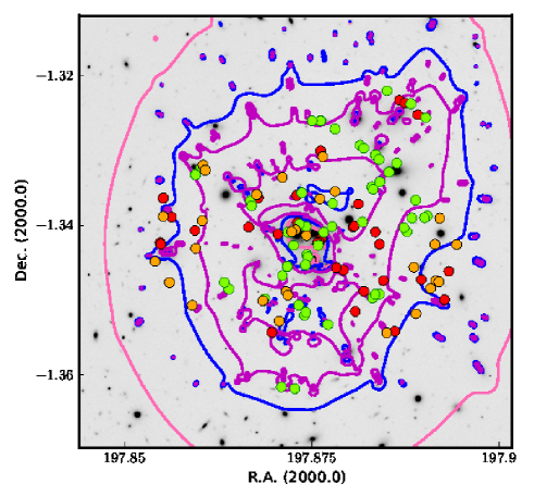
Figure 1: Magnification map of A1689 overlaid on top of an HST ACS image of the cluster. The $\Delta m=1,2,3$ mag (pink, blue, magenta) contours are shown for a source at $z=2$. The green (orange) circles indicate the positions of strongly lensed galaxies with spectroscopic redshifts and time delays below (above) 5 years. Red points indicate strongly lensed sources with photometric redshifts.

Table 1: Parameter values inferred for the dark matter clumps considered in the optimization procedure for galaxy cluster A1689. Coordinates are given in arcseconds with respect to the BGC. Error bars correspond to 1$\sigma$ confidence level as inferred from the MCMC optimization. The model has a total of 33 free parameters. Values in brackets are not optimized.

Clump	RA	DEC	$e$	$\theta$	$r_{\rm core}$ (kpc)	$r_{\rm cut}$ (kpc)	$\sigma$ (km s-1)
Clump 1	$0.5^{+0.2}_{-0.2}$	$-8.5^{+0.4}_{-0.4}$	$0.21^{+0.01}_{-0.01}$	$90.4^{+1.2}_{-1.1}$	$101.2^{+4.6}_{-4.0}$	[1515.7]	$1445.5^{+16.0}_{-14.7}$
Clump 2	$-70.7^{+1.3}_{-1.6}$	$49.1^{+3.0}_{-3.6}$	$0.77^{+0.04}_{-0.05}$	$78.6^{+2.6}_{-2.6}$	$67.9^{+8.0}_{-5.8}$	[501.0]	$647.1^{+2.1}_{-4.9}$
BCG	$-1.1^{+0.3}_{-0.2}$	$0.1^{+0.4}_{-0.4}$	$0.48^{+0.04}_{-0.04}$	$66.0^{+6.9}_{-6.3}$	$5.3^{+1.1}_{-1.1}$	$130.8^{+37.2}_{-36.2}$	$441.7^{+11.6}_{-12.2}$
Galaxy 1	[49.1]	[31.5]	$0.70^{+0.10}_{-0.15}$	$113.6^{+7.2}_{-9.8}$	$25.6^{+3.0}_{-3.4}$	$161.2^{+13.3}_{-21.9}$	$262.8^{+12.1}_{-16.6}$
Galaxy 2	$-45.7^{+0.4}_{-0.7}$	$31.6^{+0.8}_{-0.9}$	$0.80^{+0.05}_{-0.04}$	$45.5^{+2.1}_{-2.1}$	$17.6^{+1.8}_{-3.0}$	$182.8^{+5.2}_{-9.7}$	$425.6^{+21.5}_{-28.4}$
L∗ elliptical galaxy	…	…	…	…	[0.15]	$54.5^{+3.7}_{-6.7}$	$154.6^{+5.3}_{-3.4}$

Table 2: Parameter values inferred for the dark matter clump and the scaling relation considered in the optimization procedure for galaxy cluster A2204. Coordinates are given in arcseconds with respect to the BGC. Error bars correspond to 1$\sigma$ confidence level as inferred from the MCMC optimization. The model has a total of 5 free parameters. Values in brackets are not optimized.

Clump	RA	DEC	$e$	$\theta$	$r_{\rm core}$ (kpc)	$r_{\rm cut}$ (kpc)	$\sigma$ (km s-1)
Clump 1	[0.0]	[0.0]	$0.38^{+0.18}_{0.14}$	$127.64^{+5.07}_{6.63}$	$54.64^{+18.05}_{22.34}$	[1000.0]	$933.47^{+160.66}_{167.06}$
L∗ elliptical galaxy	…	…	…	…	[0.15]	[45]	$203.30^{+24.05}_{28.94}$

For investigating the power of lensed Type Ia SNe observations for constraining cluster models we are also studying cluster A2204 at redshift $z$ = 0.1524. For this cluster only one multiply lensed image system at $z=1.06$ is known, making it much less constrained than A1689. The mass model for this cluster consists of one main potential, describing the smooth cluster potential, and 34 cluster member galaxy potentials. All potentials are described by PIEMD profiles and the model has a total of 5 free parameters: the ellipticity, $e$, position angle, $\theta$, core radius, $r_{\rm core}$, and velocity dispersion, $\sigma$, of the main potential as well as the mass-luminosity scaling relation for the cluster galaxies, $L^{*}\sigma$ (compare Table 2, for details see Richard et al. 2010).

LENSTOOL is a software package for modeling mass distributions of galaxies and clusters in the strong and weak lensing regime (Jullo et al. 2007, http://www.oamp.fr/cosmology/lenstool/). Monte Carlo Markov Chains (MCMC) are used to constrain the free parameters of the cluster model derived from observational data of the background galaxies. The output contains a chain sampling the probability distribution of parameter values, each of which corresponds to a specific model realization. The density of parameter values gives a measure of the corresponding probability distribution for the parameters and can be used to estimate the errors of the corresponding parameters. For each of the realizations, the magnification and time delay function at any given position behind the cluster, can be computed.

Assuming that we observe the magnification or time delay of a multiply imaged SN, we are able to rule out all realizations that do not agree with these (simulated) additional constraints. By comparing the remaining realizations to the original chain, we are then able to judge how powerful the additional constraints are in constraining the cluster potential.

3 Supernovae behind clusters

To investigate how efficient massive galaxy clusters are for detecting distant SNe and putting constraints on cluster modeling or cosmology, a good estimate on how many SNe behind the cluster that can be expected during a given survey time is needed. For example, for a 5 year monthly survey of one very massive A1689-like cluster with HAWK-I, it has been shown that the total number of SNe expected in the background galaxies is on the order of 40–70 SNe, out of which approximately 20–30 are SNe Ia (depending on the underlying rates estimate for the various SN types, see Paper II).

For the purpose of studying time delays using galaxy cluster A1689, we focus primarily on potential SN explosions in the 24 known multiply lensed background galaxies with spectroscopic redshifts. Ten multiply imaged galaxies with photometric redshifts only are not taken into consideration to avoid additional sources of error due to uncertainties in photometric redshifts. Furthermore, with more data being collected, new multiple image systems might be detected. The numbers we present below should therefore be considered as lower limits.

Since the rate of SNe is expected to be coupled to the star-formation rate (SFR) in these galaxies, we use rate predictions for the strongly lensed systems derived from local estimates of the SFR. As the UV luminosity is dominated by the most short-lived stars, it is closely related to star formation. Thus, we use $L_{2800}$, the flux at rest-frame $\lambda_{\rm eff}=2800$ Å (redshifted to optical bands) as a tracer of the SFR in the strongly lensed galaxies. Since there are very deep HST observations of A1689 with multiple filters, these estimates are remarkably precise.

The absolute $L_{2800}$ magnitude is derived after taking into account the distance modulus, K-corrections, extinction and lensing magnification from the cluster model. Finally, we use the relation between $L_{2800}$ and SFR from Dahlén et al. (2007) to relate the flux to star formation,

$${\rm SFR}\left(M_{\odot}{\rm yr}^{-1}\right)=L_{2800}\left({\rm erg\cdot s}^{-1}{\rm Hz}^{-1}\right)\times\left(7.0\cdot 10^{27}\right)^{-1}\,.$$ (1)

The expected rate for core collapse SNe is calculated from

$$r_{\rm CC}(z)=k^{50}_{8}\times{\rm SFR}(z)\,,$$ (2)

where $k^{50}_{8}=0.007M^{-1}_{\odot}$ is estimated using a Salpeter IMF and a progenitor mass range of between 8 and 50 solar masses. For SNe Ia, we assume that the rate has two components, one proportional to the SFR and one proportional to stellar mass, according to the model of Scannapieco $\&$ Bildsten (2005). The rate is given by

$$r_{\rm Ia}(t)=A\cdot{\rm SFR}(t)+B\cdot M(t)\,.$$ (3)

The mass, $M$, of individual galaxies are calculated using mass-to-light ratios from Bell et al. (2003). The resulting rates for core collapse SNe and SNe Ia in multiply lensed background galaxies with spectroscopic redshifts and predicted time delays below 5 years are summarized in Table 3. In total, we expect $\sim$ 0.6 core collapse SNe and $\sim$ 0.05 SNe Ia per year to explode in the known multiply imaged galaxies with spectroscopic redshifts.

Table 3: All image pairs of multiply lensed background galaxies with spectroscopic redshift and a predicted time delay of less than 5 years. Column 3 gives the predicted time delay between the images. A negative time-delay indicates that image 2 will occur before image 1. Columns 4 and 5 give the predicted magnification for image 1 and image 2, respectively. In column 6 and 7 our rate estimates are shown for core collapse SNe and SNe Ia, respectively. Columns 8–14 indicate the detectability of a lensed SN for the different SN types assuming a limiting magnitude of 25.25 mag (Vega) in F140W, e.g. in a survey using 1/3 orbit with the HST/WFC3 instrument (compare with Fig. 2). Errors are given as one sigma.

Images	$z_{\rm spec}$	$\Delta t$	$\Delta m_{1}$	$\Delta m_{2}$	$r_{\rm CC}$ $\times$ $10^{2}$	$r_{\rm Ia}$ $\times$ $10^{3}$	Detectable SN types
		(d)	(mag)		(yr-1)		Ia	IIP	IIL	IILb	IIn	Ib/c	HN
1.1 + 1.2	3.04	$-83.2^{+76.9}_{-69.4}$	$3.80^{+0.30}_{-0.29}$	$5.58^{+1.21}_{-0.74}$	$2.07^{+1.07}_{1.04}$	$1.32^{+0.68}_{0.66}$	y	y	y	y	y	y	y
1.3 + 1.6	3.04	$1248.2^{+135.5}_{-148.9}$	$2.12^{+0.05}_{-0.05}$	$0.88^{+0.08}_{-0.07}$	…	…	y				y
1.4 + 1.5	3.04	$-139.4^{+87.7}_{-79.7}$	$2.85^{+0.07}_{-0.06}$	$1.88^{+0.05}_{-0.04}$	…	…	y			y	y		y
2.2 + 2.3	2.53	$-163.0^{+77.7}_{-72.2}$	$2.97^{+0.07}_{-0.06}$	$2.01^{+0.05}_{-0.04}$	$1.74^{+0.85}_{0.85}$	$1.12^{+0.52}_{0.53}$	y		y	y	y	y	y
2.4 + 2.5	2.53	$1072.8^{+119.4}_{-132.0}$	$2.07^{+0.05}_{-0.05}$	$1.00^{+0.07}_{-0.07}$	…	…	y			y	y		y
4.1 + 4.2	1.16	$575.6^{+63.7}_{-64.9}$	$2.96^{+0.04}_{-0.04}$	$2.85^{+0.05}_{-0.05}$	$0.44^{+0.16}_{0.16}$	$0.28^{+0.10}_{0.10}$	y	y	y	y	y	y	y
5.1 + 5.2	2.64	$-31.2^{+17.6}_{-16.6}$	$3.54^{+0.08}_{-0.08}$	$2.82^{+0.07}_{-0.07}$	$0.97^{+0.43}_{0.43}$	$0.65^{+0.27}_{0.27}$	y	y	y	y	y	y	y
6.1 + 6.2	1.15	$70.8^{+166.5}_{-170.4}$	$2.81^{+0.04}_{-0.04}$	$2.95^{+0.12}_{-0.09}$	$0.45^{+0.21}_{0.21}$	$6.51^{+5.50}_{5.50}$	y	y	y	y	y	y	y
6.1 + 6.3	1.15	$1759.3^{+237.3}_{-249.5}$	$2.81^{+0.04}_{-0.04}$	$3.69^{+0.74}_{-0.44}$	…	…	y	y	y	y	y	y	y
6.1 + 6.4	1.15	$222.8^{+145.5}_{-161.3}$	$2.81^{+0.04}_{-0.04}$	$3.30^{+0.56}_{-0.33}$	…	…	y	y	y	y	y	y	y
6.2 + 6.3	1.15	$1680.8^{+262.3}_{-250.1}$	$2.96^{+0.11}_{-0.10}$	$3.69^{+0.74}_{-0.44}$	…	…	y	y	y	y	y	y	y
6.2 + 6.4	1.15	$157.3^{+113.0}_{-119.9}$	$2.95^{+0.11}_{-0.10}$	$3.30^{+0.56}_{-0.33}$	…	…	y	y	y	y	y	y	y
6.3 + 6.4	1.15	$-1526.1^{+281.8}_{-286.3}$	$3.73^{+0.73}_{-0.44}$	$3.31^{+0.56}_{-0.32}$	…	…	y	y	y	y	y	y	y
7.2 + 7.3	4.87	$645.0^{+96.0}_{-82.3}$	$1.77^{+0.06}_{-0.07}$	$0.31^{+0.13}_{-0.13}$	$13.04^{+6.06}_{6.08}$	$8.34^{+3.70}_{3.71}$
10.2 + 10.3	1.83	$1376.2^{+143.0}_{-148.6}$	$2.49^{+0.08}_{-0.08}$	$0.16^{+0.12}_{-0.12}$	$5.42^{+2.48}_{2.47}$	$4.31^{+1.58}_{1.57}$	y			y	y		y
12.2 + 12.3	1.83	$63.1^{+13.0}_{-12.9}$	$3.69^{+0.06}_{-0.06}$	$7.03^{+1.05}_{-0.61}$	$0.68^{+0.32}_{0.32}$	$0.42^{+0.20}_{0.20}$	y	y	y	y	y	y	y
14.1 + 14.2	3.40	$-236.8^{+14.1}_{-17.2}$	$4.76^{+0.39}_{-0.25}$	$2.92^{+0.06}_{-0.06}$	…	…	y			y	y		y
15.1 + 15.3	1.82	$888.6^{+138.8}_{-139.3}$	$2.61^{+0.08}_{-0.08}$	$0.74^{+0.14}_{-0.13}$	$0.91^{+0.42}_{0.42}$	$0.56^{+0.26}_{0.26}$	y			y	y		y
17.1 + 17.2	2.66	$-78.8^{+24.6}_{-20.8}$	$3.21^{+0.14}_{-0.15}$	$1.40^{+0.09}_{-0.09}$	$15.13^{+6.21}_{6.19}$	$10.92^{+3.84}_{3.82}$	y			y	y		y
19.1 + 19.5	2.60	$1507.0^{+89.5}_{-92.0}$	$2.40^{+0.06}_{-0.06}$	$1.02^{+0.11}_{-0.10}$	$3.58^{+1.53}_{1.53}$	$2.43^{+0.96}_{0.96}$	y			y	y		y
19.3 + 19.4	2.60	$-84.1^{+10.5}_{-12.7}$	$3.11^{+0.06}_{-0.09}$	$5.14^{+0.21}_{-0.18}$	…	…	y	y	y	y	y	y	y
22.1 + 22.2	1.70	$462.2^{+111.6}_{-98.7}$	$2.21^{+0.07}_{-0.05}$	$0.13^{+0.22}_{-0.20}$	$2.77^{+1.03}_{1.06}$	$2.16^{+0.68}_{0.70}$	y			y	y		y
24.2 + 24.3	2.63	$-1029.2^{+157.2}_{-148.9}$	$4.81^{+1.14}_{-0.61}$	$2.96^{+0.05}_{-0.05}$	$0.93^{+0.43}_{0.42}$	$0.62^{+0.27}_{0.26}$	y	y	y	y	y	y	y
24.2 + 24.4	2.63	$-1364.2^{+198.6}_{-196.9}$	$4.81^{+1.14}_{-0.61}$	$2.83^{+0.09}_{-0.08}$	…	…	y	y	y	y	y	y	y
24.3 + 24.4	2.63	$-343.0^{+169.7}_{-164.7}$	$2.96^{+0.05}_{-0.05}$	$2.83^{+0.09}_{-0.08}$	…	…	y	y	y	y	y	y	y
29.2 + 29.3	2.57	$1017.8^{+162.5}_{-170.9}$	$3.04^{+0.05}_{-0.05}$	$4.90^{+1.27}_{-0.66}$	$0.71^{+0.40}_{0.37}$	$0.53^{+0.27}_{0.26}$	y	y	y	y	y	y	y
29.2 + 29.4	2.57	$136.7^{+147.5}_{-140.0}$	$3.04^{+0.05}_{-0.05}$	$2.78^{+0.08}_{-0.08}$	…	…	y	y	y	y	y	y	y
29.3 + 29.4	2.57	$-881.6^{+179.0}_{-168.9}$	$4.90^{+1.27}_{-0.66}$	$2.78^{+0.08}_{-0.07}$	…	…	y	y	y	y	y	y	y
30.1 + 30.2	3.05	$-27.3^{+186.6}_{-191.8}$	$2.71^{+0.09}_{-0.07}$	$4.89^{+0.99}_{-0.52}$	$3.41^{+2.48}_{2.44}$	$2.40^{+1.68}_{1.65}$	y			y	y		y
30.1 + 30.3	3.05	$1022.6^{+339.4}_{-316.4}$	$2.71^{+0.09}_{-0.08}$	$4.86^{+1.10}_{-0.70}$	…	…	y			y	y		y
30.2 + 30.3	3.05	$1052.7^{+183.1}_{-166.8}$	$4.89^{+0.98}_{-0.53}$	$4.86^{+1.09}_{-0.70}$	…	…	y	y	y	y	y	y	y
32.1 + 32.2	3.00	$350.1^{+90.7}_{-91.6}$	$2.15^{+0.05}_{-0.06}$	$2.97^{+0.07}_{-0.07}$	$4.38^{+1.75}_{1.75}$	$3.07^{+1.07}_{1.07}$	y			y	y		y
32.3 + 32.4	3.00	$759.0^{+98.3}_{-98.9}$	$2.19^{+0.06}_{-0.05}$	$1.29^{+0.06}_{-0.05}$	…	…	y			y	y
35.1 + 35.3	1.91	$1246.8^{+95.3}_{-95.9}$	$2.69^{+0.06}_{-0.06}$	$0.97^{+0.15}_{-0.14}$	$2.54^{+1.07}_{1.07}$	$1.65^{+0.67}_{0.67}$	y			y	y		y
36.1 + 36.2	3.01	$-45.4^{+18.2}_{-21.0}$	$4.92^{+0.17}_{-0.16}$	$4.52^{+0.13}_{-0.14}$	$0.06^{+0.03}_{0.03}$	$0.04^{+0.02}_{0.02}$	y	y	y	y	y	y	y

To calculate the properties of the lens systems, i.e., masses and SFRs, we use available observations in the HST/ACS optical filters (f435w, f475w, f555w, f625w, f775w, f850lp), as well as HST/NICMOS IR filters (f110w, f160w) from Richard et al. (in preparation).

Using the cluster model to calculate magnifications, we can now investigate the observability of such systems. In order to be observable, not only must the time delay be smaller than the survey length (here assumed to be 5 years) but also the luminosity of both images must lie above the observation threshold. Here we have chosen a magnitude limit of 25.25 mag (Vega) in F140W, corresponding to what could be achieved, e.g., with 1/3 orbit with the HST/WFC3. In Fig. 2, the predicted light curves for SNe of Type Ia and IIP are shown. As can be seen, nearly all SNe Ia exploding in one of the known multiply lensed background galaxies would be bright enough to be observable, while about half of the SNe IIP, mostly at lower redshift and with high magnification, would lie above the luminosity threshold. Columns 8–14 in Table 3 indicate which SN type would be observable for each image combination producing appropriate time delays.

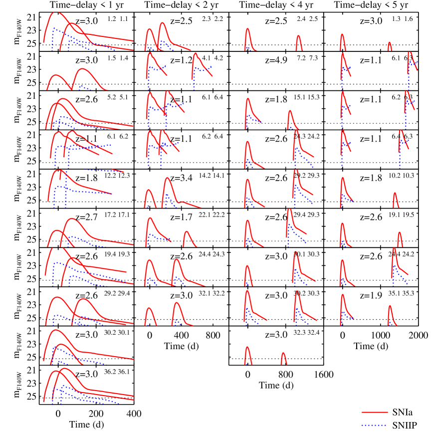
Figure 2: Simulated light curves of SNe Ia and IIP for pairs of images of strongly lensed galaxies behind A1689. Only pairs with time-delay $<$ 5 years are shown. Additional information on different image pairs labeled by, e.g., 1.2 and 1.1 in the top right corner of each sub panel, can be found in Table 3. The dashed line indicates an expected magnitude limit 25.25 (Vega) in F140W.

4 Cluster model constraints

When modeling the potential of a cluster as described in Sect. 2, information on the position of the multiple images is used to optimize the free parameters. In general, the addition of a constant surface density $\kappa_{\rm c}$ to a lens potential leaves the resulting image positions of a system unchanged. This is known as the mass sheet degeneracy. In the case of A1689, due to its large number of known multiply imaged systems at different redshifts, this degeneracy is broken. However, for galaxy clusters with only very few observed lens systems, this degeneracy can be problematic. The detection of a SN Ia behind a cluster offers a direct way of constraining the lens potential. Due to the standard candle nature of SNe Ia, see Goobar & Leibundgut (2011) for a recent review, the information on the absolute magnitude can be used to measure the magnification at the position of the SN and compare it to mass model predictions. One would then be able to rule out realizations producing deviant magnifications. The precision of the magnification measurements are ultimately limited by the intrinsic scatter in the brightness of SNe Ia after corrections for lightcurve shape and color, about 0.1 mag in the rest-frame optical wavelength region (Conley et al. 2011). We do not anticipate any additional sources of error due to the cluster in the line of sight. E.g., observing at near-IR wavelengths ensures that corrections from dust in the (low-$z$) cluster are small, especially since galaxy clusters are relatively dust-free environments, see Dawson et al. (2009) and references therein. Thus, a SN Ia exploding in any of the background galaxies behind the cluster could be used to put constraints on the lensing potential. As discussed in Paper II, we expect to detect $\sim$ 20–30 SNe Ia (depending on the underlying rates estimates) to be detectable, e.g., in a 5 year monthly survey at VLT. In order to assess the power of this method, we investigate the strength of the correlation between the optimized model parameters and the magnification for different positions behind the cluster.

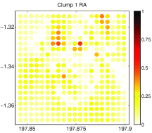
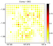
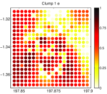
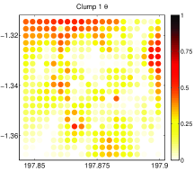
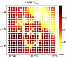
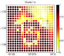
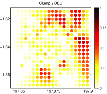
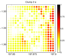
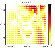
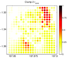
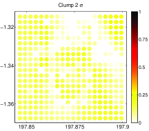
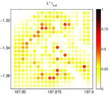
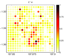
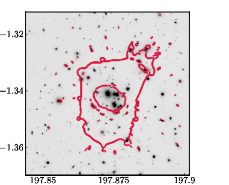
Figure 3: Correlations between the predicted magnification as a function of image position for a source at redshift $z=2$ and the input parameters which are optimized in the model for A1689 (compare Table 1) in a field of view $\pm$ 100 arcseconds around the cluster center. Correlations are given as the absolute values of the correlation coefficients. A high value (close to 1; dark red) indicates that that the magnification for an image at the given position will display large variations when the input parameter is varied. Being able to measure the absolute magification at this image position, using e.g. SNe Ia observations, will thus make it possible to improve the constraints on the cluster parameter. If the correlation is low (close to 0; light yellow), we do not expect magnification information to significantly improve the current constraint on the cluster parameter at hand. The strongest correlations and best possibility of improving the model once a SN Ia is observed, are the ellipticity, $e$, core radius, $r_{\rm core}$, and velocity dispersion, $\sigma$, of the main lensing potential. The last panel shows an ACS image of the cluster overlaid with the critical lines for $z=2$. The FOV in all panels is identical with Fig. 1.

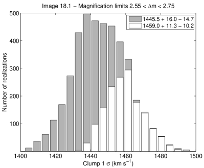
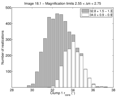
Figure 4: Possible constraints on the model parameters describing the velocity dispersion (left) and core radius (right) of the main dark matter clump of A1689 using information on the magnification from a SN Ia observed in the multiply lensed background galaxy image 18.1 at $z$ = 1.82. The shaded bars represent the parameter distribution from all realizations while the unfilled bars give the parameter distribution considering only realizations which reproduce the observed magnification within $\pm$ 0.1 mag.

Figure 3 shows the absolute value of the correlation coefficients for the predicted magnification and the free input parameters as a function of position for an image at redshift $z=2$. The parameters shown are those describing the two dark matter clumps (Clump 1 and Clump 2) and the cluster galaxy scaling relations ($L^{*}r_{\rm cut}$ and $L^{*}\sigma$) in the model of A1689. A value close to 1 implies a very strong correlation while a correlation coefficient close to 0 implies no correlation. As can be seen in Fig. 3, the free parameters differ in the strength of their correlation with the predicted magnification both with each other and the position behind the cluster. The dependence of the correlation strength on redshift is very weak. In general, of all 33 free optimized parameters, the ones which show the strongest correlations and therefore the possibility of improving the model once a SN Ia is observed, are the ellipticity, $e$, core radius, $r_{\rm core}$, and velocity dispersion, $\sigma$, of the main lensing potential (Clump 1). Other parameters, like the corresponding parameters for the cluster galaxies and the position of the main lensing potentials show a weaker correlation and can probably not be further constrained using SN Ia observations in the case of A1689.

Figure 4 shows an example of how the model parameters could be constrained if the magnification of an image is known to a precision of 0.1 mag. In this example we asssume a SN Ia observed in the multiply-lensed image 18.1 with spectroscopic redshift $z$ = 1.82 under the most favorable conditions. Since this image does not have a counter image with a time delay below five years, it is not included in Table 3. At the position of this image, there are strong correlations between the model parameters and the predicted magnification of this image. The correlation coefficient for the velocity dispersion and core radius of the main clump (Clump 1) are 0.84 and 0.87, respectively. As can be seen in Figure 4, the possible constraints on $\sigma$ for the main lensing potential improve from $\sim 1\%$ to $\sim 0.7\%$, while the corresponding numbers for $r_{\rm core}$ are $\sim 4.5\%$ and $\sim 2.6\%$. Thus, adding only one constraint from the observed magnification of a SN Ia, the constraints on the model parameters for this already very well constrained cluster model of A1689 (114 multiple images and 24 spectroscopic redshifts), improve by almost a factor of 2. It should however be noted, that the possible constraints from this image should be seen as a best case scenario, as the correlations for other systems are typically weaker, with median absolute correlation coefficient values in a FOV extending $\pm$ 100 arcseconds around the center of the cluster at $z=2$ of 0.67 and 0.71 for the velocity dispersion of the main clump (Clump 1) and its core radius, respectively. Since we are expecting $\sim 5$ SNe Ia exploding in all background galaxies per year, we would be able to obtain a combined constraint from such observations of the magnification at several positions behind the cluster.

This technique might prove to be even more interesting for testing the mass modeling of other less constrained galaxy clusters. To evaluate the power of the method, we investigate cluster A2204 with only one known multiply lensed image system, making it much less constrained than A1689, which we have been focusing on so far. Again, we investigate the correlations of the optimized free parameters with the resulting magnifications. The correlation strengths for a grid of image positions $\pm$ 100 arcseconds around the cluster center at redshift $z=1$ is shown in Fig. 5. Similarly to the case of A1689, the strongest correlations are found for $\sigma$ and $r_{\rm core}$ of the main potential with the median absolute correlation coefficient values in the FOV shown in Fig. 5 at redshift $z=1$ being 0.96 and 0.87, respectively. It is notable that these correlations are rather weak in the central regions of the cluster potential, which is constrained through the location of the known multiple images.

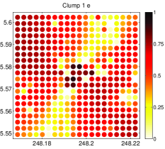
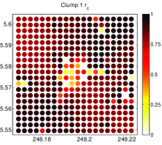
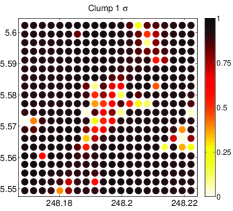
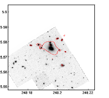
Figure 5: Correlations between the predicted magnification of an image as a function of image position for a source at redshift $z=1$ and the different input parameters which are optimized in the model for A2204 (compare Table 2 and Fig. 3) in a field of view $\pm$ 100 arcseconds around the cluster center. Correlations are given as the absolute values of the correlation coefficients. The last panel shows an ACS image of the cluster overlaid with the critical lines for $z=1$.

In Figure 6, we show the constraints on these parameters from the magnification of a hypothetical SN Ia with $z=1$ close to the position of the known lensed image 1.1 measured with an uncertainty of $\pm$ 0.1 mag. The values of the correlation coefficients for $\sigma$ and $r_{\rm core}$ of the main clump (Clump 1) are 0.90 and 0.79, respectively. In this case, the constraints on the velocity dispersion for the main lensing potential improve from $\sim 17\%$ to $\sim 3.5\%$, while the corresponding constraint for the core radius goes from essentially unconstrained (with a forced upper limit from observations) to $\sim 25\%$. Thus, observations of SNe Ia behind galaxy clusters promise to be a powerful tool in constraining their overall lens potential and thereby the properties of the dark matter component.

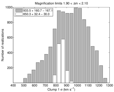
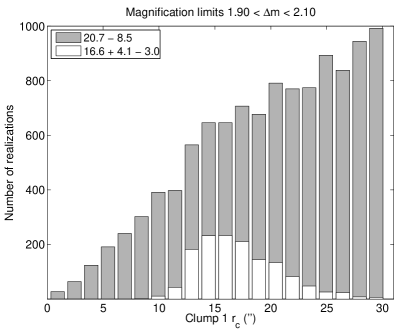
Figure 6: Possible constraints on the model parameters describing the velocity dispersion (left) and core radius (right) of the main dark matter clump for A2204 using information on the magnification from a SN Ia observed in the image. The shaded bars represent the parameter distribution from all realizations while the unfilled bars give the parameter distribution considering only realizations which reproduce the observed magnification within $\pm$ 0.1 mag.

5 Measuring the Hubble constant

It has earlier been suggested to use time delays from multiply-lensed sources to measure the Hubble constant (e.g., Refsdal 1964). For a strong lens system, the arrival time of an image at angular position $\@vec{\theta}$ relative to the unlensed case for a corresponding source position $\@vec{\beta}$ is given by

$$\Delta t=\frac{1+z_{\rm L}}{c}\frac{D_{\rm L}D_{\rm S}}{D_{\rm LS}}\left[\frac{(\@vec{\theta}-\@vec{\beta})^{2}}{2}-\psi(\@vec{\theta})\right],$$ (4)

where $z_{\rm L}$ is the redshift of the lens, $D_{\rm L}$, $D_{\rm S}$, and $D_{\rm LS}$ are, respectively, the angular diameter distances to the lens, to the source, and from the lens to the source, and $\psi(\@vec{\theta})$ is the lens potential.

Since the ratio of the angular diameter distances scales inversely with the Hubble constant, $D\equiv\frac{D_{\rm L}D_{\rm S}}{D_{\rm LS}}\propto H_{0}^{-1}$. By modeling the lens potential, $\psi(\@vec{\theta})$, and the source position, $\@vec{\beta}$, one can use time delay measurements from strongly lensed systems to estimate the Hubble constant.

There is also a dependence on $D$ from other cosmological parameters, such as $\Omega_{\rm M}$ and $\Omega_{\Lambda}$, although this dependence is much weaker than that on the Hubble constant (e.g., Bolton $\&$ Burles 2003; Coe & Moustakas 2009; Suyu et al. 2010).

Due to the transient nature of SNe, the observed time delay from SN light curves can be determined with high precision, typically on the order of less than a few days. To improve the constraints on $H_{0}$ it is thus important to be able to narrow down the errors of the lens potential. Here we investigate the constraints on $H_{0}$ possible when observing a SN in one of the known multiply-imaged background galaxies of A1689 with predicted time delays below 5 years and spectroscopic redshifts. Summing up our SN rate estimates (given in Table 3), we expect an average total of 3 SNe exploding in those galaxies during a survey time of 5 years. The effective number of strongly lensed SNe which are observable, will depend on the survey properties. For a five year monthly survey using the HST/WFC3, we would expect to detect approximately 1 strongly lensed SN in these galaxies. However, one should keep in mind that there are 10 more known strong lensing systems behind A1689, consisting of 30 images, which have not been included in this study since they have photometric redshifts only. Furthermore, as observations of this massive cluster continue, additional multiply lensed systems might be discovered (Coe & Moustakas 2009).

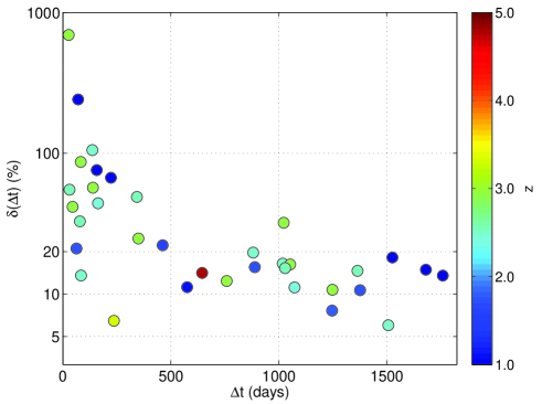
Figure 7: Predicted time delays in days and percentual one sigma errors for all the image pairs of multiply imaged background galaxies with spectroscopic redshift and time delay smaller than five years behind A1689. The color of the markers indicates the redshift of the systems.

From the different realizations of the cluster modeling, we get a prediction with error estimates for the time delays between image pairs in the known multiply lensed background galaxies. These errors depend on the positions of the image pairs. As can be seen in Fig. 7, for more than half of the image pairs with predicted time delays below five years and spectroscopic redshift, the corresponding errors are below 20%. For several systems the time delay precision from the model lies around 10% and below. Eventually combining constraints from several strongly lensed SNe, would allow the value of the Hubble constant to be determined with high precision. Thus, nominally, to match the current $\sim 3\%$ accuracy of the local measurements of $H_{0}$ (Riess et al. 2011), about ten massive clusters should be monitored for five years. Although it may seem like a rather large time investment in telescope time to match a result already at hand, we emphasize the importance of a non-local test of the universal Hubble scale, a key test in cosmology.

In the case of a lensed SN Ia, we can use the information on the absolute magnification to rule out realizations that predict magnifications outside the range allowed by observations. With this extra information, we might be able to further constrain the time delay error from the lens model. Therefore, we check for correlations between the predicted magnification of the images in a system and the time delay between the images. While many systems show no or only weak correlations between magnifications and time delay, there are a few more promising systems.

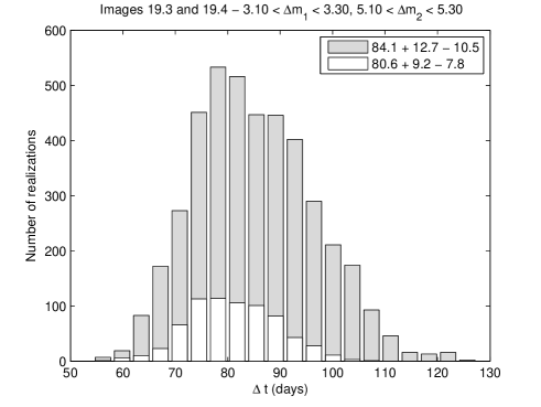
Figure 8: Constraints on the time delay between images 19.3 and 19.4 at $z$ = 2.60 behind A1689 using the magnification of both images. In the shaded histogram the time delay distribution from the complete Monte Carlo Markov Chain is shown. The unfilled histogram shows the distribution after the cuts due to magnification constraints. Errors are given as one sigma.

Figure 8 shows an example for the cuts in time delay error which can be made using magnification constraints from a lensed SN Ia in background galaxy 19. In this case, the errors on the time delay between images $19.3$ and $19.4$ can be reduced from $\approx^{+15.1}_{-12.5}$ to $\approx^{+11.4}_{-9.7}$ %.

As discussed in Sect. 4, the additional model constraints from a measurement of the magnification by using the standard candle nature of SNe Ia are only modest for a well constrained cluster as A1689. However, such a constraint would prove much more valuable in the case of a time delay measured in a less constrained cluster as it could break the degeneracy between the mass profile and the Hubble constant (Oguri & Kawano 2003).

6 Discussion and Conclusions

A SN Ia exploding in any of the background galaxies of a cluster will give an absolute measure of the magnification at that point and can therefore potentially be used to constrain the mass modeling of the cluster. For cluster A1689, which we have been focusing on in this study, the cluster potential is already very well modelled. However, such an additional constraint from one or more lensed SNe could help to improve the cluster model further by reducing parameter uncertainties. For less constrained galaxy clusters, this technique proves to be even more interesting. Using the magnification information from a single SN Ia behind cluster A2204 can be a powerful tool to narrow down the model parameters of the dark matter halo component.

Since SNe are point-like sources for a limited period, microlensing from stars in a cluster galaxy close to the line of sight might in principle have an important effect on the magnification and thus affect the possible constraints on the large scale mass model from SNe Ia. However, it has been concluded (Oguri & Kawano 2003) that this effect should only cause small deviations. Microlensing events caused by massive compact halo objects (MACHOs) in the intracluster medium might unambiguously be identified in SN light curves. Thus any modulation of the light curve shape, or lack thereof, can put limits on the mass fraction of the cluster mass in the form of $10^{-7}<M/M_{\odot}<10^{-4}$ MACHOs (Kolatt & Bartelmann 1998).

In the case of a SN exploding in one of the known multiply lensed background galaxies, there is a good chance of observing multiple images of the SN and determine the observed time delay with high precision. The intrinsically brighter SNe, e.g. SNe Ia and SNe IIn, should in principle be detectable in essentially all of the systems. However, for SNe IIP, which are expected to be the most common SN type, the magnification is only strong enough for them to become observable in about half of the cases.

Due to the well constrained mass model for galaxy cluster A1689, SN time delays can be used as an independent measure on the Hubble parameter at high redshift. In case of a SN Ia, the magnification might also be used as a constraint to further improve the error in the time delay predicted by the lensing model. Another advantage with using a cluster with a well constrained mass model is the possibility of predicting subsequent images, if a SN behind the cluster is observed.

It is quite exciting that CLASH, a cluster monitoring multi-cycle program is currently been pursued (Postman et al. 2011). However, the strategy in the CLASH program is tuned for finding and accurately studying SNe Ia in the parallel fields, i.e., in the low magnification region. Much of the observations of the cluster cores are done in optical and UV filters, where high-$z$ SNe would not be detectable. Furthermore, the cluster fields are only monitored for 2-4 months making the search for multiple images practically impossible, especially considering the time dilation $(1+z)=$2-4.5 in the lensed SN lightcurves.

Corroborating the value of $H_{0}$ found in the local universe could provide crucial support to our cosmological picture. On the other hand, a discrepancy would falsify the accepted scenario and shed new light into the dark matter and dark energy puzzles. Since strongly lensed SNe involve both angular diameter and luminosity distances ($d_{\rm A}$ and $d_{\rm L}$), such systems provide an unique chance to probe the distance reciprocity relation, $d_{\rm L}=(1+z)^{2}d_{\rm A}$. Any violation of this relation would indicate either the existence of unaccounted astrophysical systematic effect affecting one of the distance measure but not the other, or that the Universe is not described by the standard cosmological model. Specifically, a violation could indicate that the Universe is described by a non-metric theory of gravity or a theory in which light does not travel on unique null geodesics. Current tests of $d_{\rm L}/d_{\rm A}$ are restricted to $z<1$ (e.g., Lampeitl et al. 2010) and have $>20\%$ uncertainties.