Probing Cosmology with Weak Lensing Minkowski Functionals

Abstract

In this paper, we show that Minkowski Functionals (MFs) of weak gravitational lensing (WL) convergence maps contain significant non-Gaussian, cosmology-dependent information. To do this, we use a large suite of cosmological ray-tracing N-body simulations to create mock weak WL convergence maps, and study the cosmological information content of MFs derived from these maps. Our suite consists of 80 independent $512^{3}$ N-body runs, covering seven different cosmologies, varying three cosmological parameters $\Omega_{m}$, $w$, and $\sigma_{8}$ one at a time, around a fiducial $\Lambda$CDM model. In each cosmology, we use ray-tracing to create a thousand pseudo-independent 12 ${\rm deg}^{2}$ convergence maps, and use these in a Monte Carlo procedure to estimate the joint confidence contours on the above three parameters. We include redshift tomography at three different source redshifts $z_{s}=1,1.5,2$, explore five different smoothing scales $\theta_{G}=1,2,3,5,10$ arcmin, and explicitly compare and combine the MFs with the WL power spectrum. We find that the MFs capture a substantial amount of information from non-Gaussian features of convergence maps, i.e. beyond the power spectrum. The MFs are particularly well suited to break degeneracies and to constrain the dark energy equation of state parameter $w$ (by a factor of $\approx$ three better than from the power spectrum alone). The non-Gaussian information derives partly from the one-point function of the convergence (through $V_{0}$, the “area” MF), and partly through non-linear spatial information (through combining different smoothing scales for $V_{0}$, and through $V_{1}$ and $V_{2}$, the boundary length and genus MFs, respectively). In contrast to the power spectrum, the best constraints from the MFs are obtained only when multiple smoothing scales are combined.

I Introduction

Forthcoming large weak gravitational lensing (WL) surveys, such as those by the Large Synoptic Survey Telescope (LSST), will provide a growing number of cosmic shear measurements of increasing quality. This prospect poses the theoretical challenges of (i) how much statistical information could be extracted from the expected WL maps, and (ii) to what extent this information will help constrain cosmological models. The power spectrum, or equivalently the two-point correlation function, are of unquestionable importance, but are nevertheless incomplete statistical descriptions of the lensing maps. This is because gravity is non-linear, and it generates non-Gaussianity on small scales. Perhaps the most natural way to proceed and characterize non-Gaussian statistical signatures is by using higher–order poly-spectra Zaldarriaga:2002qt , or equivalently, three–point and higher–order correlation functions Bernardeau97 ; Hui99 ; T&J02 ; Takada:2003sv ; T&J04 ; Sefusatti06 ; Berge:2009xj ; Takada:2008fn ; Jain:2003tba . An interesting, and less explored alternative, originally suggested in the context of the cosmic density field gmd86 , is to utilize topological features.

As an example of this approach, the genus of different iso-density contour surfaces hgw86 ; gwm87 ; g89 ; v94 ; pkg05 has recently been measured in the Sloan Digital Sky Survey (SDSS). The genus curve—i.e. genus as a function of density threshold—was derived for both the luminous red galaxy (LRGs) and the main galaxy samples, and found to deviate from the theoretical prediction for a Gaussian random field. These deviations then allowed a testing of different galaxy formation scenarios, through their nonlinear biasing and other gravitational effects g09 ; c10 .

The genus is only one of several topological measures of iso-density surfaces (in three-dimensions) or contours (in two-dimensions), which are collectively known as the Minkowski functionals (MFs) mbw94 . The full set of MFs has been successfully applied to maps of Cosmic Microwave Background (CMB) temperature anisotropies, to probe primordial non-Gaussianity. There one compares the MFs derived from the data to those expected in standard inflationary models with Gaussian initial conditions  WMAP1 ; WMAP3 ; WMAP5 . The current constraints from the MFs on the commonly used non-Gaussianity parameter $f_{\rm NL}$ are comparable to those from the bispectrum Hikage:2008gy . However, the MFs have the additional ability to test models of the early universe with non-Gaussianity only appearing at the level of trispectrum or beyond m10 .

Motivated by these demonstrations that MFs are powerful yet simple probes of non-Gaussianity, we here perform a detailed and systematic study the MFs of the cosmic shear field and their potential use to differentiate between cosmological models. Related previous works have considered the $\Omega_{m}$–dependence of the one–point function and WL peak statistics, using ray-tracing simulations JSW00 ; BJ&VW00 , and have demonstrated the ability of WL MFs to distinguish standard cold dark matter (SCDM), open CDM and $\Lambda$CDM models Sato:2001cb ; g02 . It has also been shown that one of the MFs, the area statistic, could place strong constraints on the properties of dark energy whm09 . Finally, a recent theoretical analysis presents a perturbative description of WL MFs Munshi:2011wu .

Our work here extends the previous studies in many ways, including the scope, detail, and the level of interpretation of the results. In particular, we have run a large suite of $N$-body simulations with ray-tracing to generate WL maps for seven different cosmological models. We vary three cosmological parameters, $\Omega_{m}$, $w$, and $\sigma_{8}$, one at a time, around a fiducial model. Using our simulation suite, we are able to compute the joint confidence levels on these three parameters through a Monte Carlo procedure. We quantify in detail where these constraints come from, finding ideal combinations of galaxy source redshifts and smoothing scales. Finally, in order to isolate the non-Gaussian information, we explicitly compare and combine the constraints from the MFs with those from the WL power spectrum.

The core finding of this paper is that the MFs capture significant non-Gaussian, cosmology-dependent information. In particular, the dark energy equation of state parameter $w$ is constrained by a factor of approximately three better than from the power spectrum alone. We attribute this improvement to the MFs breaking degeneracies between $w$ and the other parameters. We also explore combinations of the three different MFs, and of the MFs with the power spectrum. This allows us to assess the amount of additional information contained in the MFs (beyond the power spectrum), and to interpret the nature of the non-Gaussian information.

The rest of this paper is organized as follows. The details of our simulations and mock WL maps are described in Section II. The basics of MFs and the algorithm to measure them from our simulated maps are described in Section III.1, while Section III.2 describes our use of the WL power spectrum. Our Monte Carlo procedure, using the maps to compute the confidence levels on the parameters, is described in Section IV, along with a discussion of the required number of pseudo-independent realizations. Section V presents our main results, showing the constraints on the cosmological parameters. Various combinations of the observables are studied: using individual MFs separately, combining MFs with the power spectrum, using redshift tomography, combining smoothing scales, using maps with and without intrinsic ellipticity noise, etc. In this section, we also compare our power-spectrum-alone constraints to the literature, and discuss several possible sources of inaccuracy, some quantified here, as well as some left for future work. Finally, in Section VI, we summarize our conclusions and the implications of this work.

II Simulation Suite and Weak Lensing Maps

II.1 N-body Simulations

The large-scale structure simulations and lensing maps were created with our new Inspector Gadget lensing simulation pipeline InspectorGadget1 ; InspectorGadget2 on the New York Blue supercomputer, which is part of the New York Center for Computational Sciences at Brookhaven National Laboratory/Stony Brook University. The center features an IBM Blue Gene/L with 36,864 CPUs and a Blue Gene/P with 8,192 CPUs. We ran a series of 80 CDM $N$-body simulations with $512^{3}$ particles each and a box size of $240h^{-1}$ Mpc. This corresponds to a three-week test run for our pipeline. We used a modified version of the public N-body code Gadget-2 Springel:2005mi , which we adapted for the Blue Gene/L and /P, and enhanced to allow the dark energy equation of state parameter $w\neq 1$, as well as to compute weak lensing related quantities, such as comoving distances to the observer. Gadget’s adjustable parameters were fine-tuned for maximum throughput on the cluster. Volker Springel kindly provided us with the initial conditions (IC) generator N-GenIC. The total linear matter power spectrum, which is an input for the IC generator, was created with the Einstein-Boltzmann code CAMB Lewis:1999bs for $z=0$, and scaled to the starting redshift of our simulations at $z=100$ following the linear growth factor. The WL maps were created, and the rest of the analysis were performed with our own proprietary codes and file formats. Up to 70TB of simulation and lensing products were stored in the process of this work.

A total of 80 N-body simulations were run, covering 7 different cosmological models in multiple runs with different random initial conditions. A total of 50 of the runs were performed in our fiducial cosmology, with parameters chosen to be {$\Omega_{m}=0.26$, $\Omega_{\Lambda}=0.74$, $w=-1.0$, $n_{s}=0.96$, $\sigma_{8}=0.798$, $H_{0}=0.72\}$. These runs all used the same input power spectrum, but a different and strictly independent realization, yielding a statistically robust set of maps, and allowing us to assess how much the use of fewer independent realizations (used in the other models) affects the results. In each of the other six cosmological models, we varied one parameter at a time, keeping the others fixed, with the following values: $\Omega_{m}=\{0.23,0.29\}$ (while $\Omega_{\Lambda}=\{0.77,0.71\}$ such that the universe stays spatially flat), $w=\{-0.8,-1.2\}$, and $\sigma_{8}=\{0.75,0.85\}$. For these six non-fiducial cosmological models we ran 5 simulations each, with a different realization of the initial conditions.

Identifier	$\sigma_{8}$	$w$	$\Omega_{m}$	$\Omega_{\Lambda}$	# of sims
Fiducial	0.798	-1.0	0.26	0.74	45
Auxiliary	0.798	-1.0	0.26	0.74	5
Om23	0.798	-1.0	0.23	0.77	5
Om29	0.798	-1.0	0.29	0.71	5
w12	0.798	-1.2	0.26	0.74	5
w08	0.798	-0.8	0.26	0.74	5
si75	0.750	-1.0	0.26	0.74	5
si85	0.850	-1.0	0.26	0.74	5

Table 1: Cosmological parameters varied in each model.

II.2 Lensing Maps

The weak lensing maps were created with a standard two-dimensional ray-tracing algorithm. We refer the reader to our previous work Kratochvil:2009wh and to InspectorGadget1 for the full description of our methodology. The code developed and used in that paper was adapted here for the Blue Gene/P and /L and parallelized to deal with the stringent memory requirements, but in its core equations it remained the same, so we will list here only the specifications as well as any changes and additions we have made.

We chose to implement the ray-tracing algorithm described in Hamana:2001vz . Earlier work with similar algorithms include Schneider:1992 ; Wambsgaans:1998 ; Jain:1999ir . The large-scale structure from the N-body simulations was output as particle positions in boxes at different redshifts, starting at redshift $z=2$. The particles were then projected onto planes perpendicularly to the planes and the central line of sight of the map. We used the triangular shaped cloud (TSC) scheme Hockney-Eastwood to place the particles on a grid on these two-dimensional density planes; the particle surface density was then converted into the gravitational potential via the Poisson equation. The algorithm then followed light rays from the observer back in cosmic time. The deflection angle, as well as the weak lensing convergence and shear were calculated at each plane for each light ray. These depend on the first and second derivatives of the potential, respectively. Between the planes, the light rays travel in straight lines. For simplicity, in this work we utilized only the convergence maps; shear maps were also created and will be used in the future.

The maps were created for $2048\times 2048$ light rays, with the lens planes spaced $80h^{-1}$Mpc apart along the line of sight. The lens planes themselves recorded the gravitational potential on a finer $4096\times 4096$ grid, to avoid losing power on small angular scales, as pointed out in Sato:2009 . We have found a similar fall-off, and therefore increased the resolution on the density planes from our previous publication Kratochvil:2009wh .

We created one thousand 12-square-degree convergence maps for each cosmology, by mixing simulations with different random initial conditions, and by randomly rotating and shifting the simulation data cubes. For the maps in each non-fiducial cosmology, lens planes mixed from all five independent N-body runs were used. In the fiducial cosmology, we created two sets of 1,000 maps. One of these sets was created from the five independent N-body runs with the same five quasi-identical initial conditions as in the non-fiducial cosmologies, and will hereafter be referred to as the “auxiliary” set. The second was created by mixing lens planes from the remaining larger ensemble of 45 independent N-body runs, and will be referred to as the “fiducial” set.

Results from the fiducial and auxiliary map sets will be compared below to verify that they do not depend on a particular set of maps and simulations. Having two independent sets will also be utilized in our Monte Carlo procedure, which involves a $\chi^{2}$–minimization. This crucially requires that the maps for which the best-fit model parameters are found are independent of the set used to compute the covariance matrix.

For simplicity, we assumed the source galaxies are confined to planes at a fixed redshift. The convergence maps were generated for three different source redshifts, $z_{s}=1,1.5$, and $2$. After the raw maps with the lensing signal were generated, ellipticity noise from the random orientations of the source galaxies was added to the maps pixel by pixel. We assumed the noise is represented by a Gaussian random field (with a top-hat filter of pixel size; or equivalently a random lattice noise model, e.g Mantz08 ). We further assumed a uniform source galaxy surface density of $n_{gal}=15$ galaxies/arcmin² on each source plane (neglecting other effects, such as shot noise from random galaxy positions, or magnification of the source galaxies) and a redshift dependent root-mean-square of the noise in one component of the shear Song and Knox (2004)

$$\sigma_{\gamma}(z)=0.15+0.035z.$$ (1)

The r.m.s. noise for a pair of pixels $\vec{x}$ and $\vec{y}$ on the convergence maps was then taken to be

$$\langle\kappa_{\rm noise}(\vec{x})\kappa_{\rm noise}(\vec{y})\rangle=\frac{\sigma_{\gamma}^{2}}{n_{gal}A}\delta_{\vec{x}\vec{y}},$$ (2)

where $\delta_{\vec{x}\vec{y}}$ is the Kronecker delta function, and $A$ is the solid angle of a pixel. The galaxy densities adopted for a single source redshift is fairly low. This lets us combine the three redshifts to employ tomography with a total $n_{gal}=45$ galaxies/arcmin², a typical value expected for galaxy surveys with the depth of LSST (e.g. LSST:2008 and Eq. (3.7) in LSST:2009pq ). Once noise in each pixel is added, we smooth the maps with a finite version of a 2D Gaussian filter, with the kernel around every pixel $\phi_{0}$,

$$W_{G}(\phi,\phi_{0})=\frac{1}{\pi\theta^{2}_{G}}\exp\left(-\frac{(\phi-\phi_{0})^{2}}{\theta_{G}^{2}}\right),$$ (3)

truncated at $6\theta_{G}$. We employ five different smoothing scales, $\theta_{G}=1,2,3,5,10$ arcmin. The smallest smoothing scale retains the most information but also the most noise. Hence, the strategy is to combine MFs with several different smoothing scales to extract additional information, despite strong correlations between maps with different $\theta_{G}$.

In Section III.2 below, we will discuss the accuracy of our simulations pipeline and the convergence power spectrum derived from the maps.

III Minkowski Functionals and Power Spectra

III.1 Minkowski Functionals

Minkowski Functionals are morphological statistics of thresholded smoothed random fields, complementary to the more familiar hierarchy of correlation functions. If the fields are strictly Gaussian, then there exist one–to–one mappings between the power spectrum and the MFs. In the weakly non-Gaussian case, one can also find an approximate map between the two statistics Hikage:2006fe , or expand the MFs perturbatively as a function of the power spectrum Matsubara:2010te ; Munshi:2011wu . In the general case, however, MFs encode information from correlation functions of arbitrarily high order, which is what makes them useful probes of non-Gaussianities. Since weak lensing convergence maps are expected to contain small scale non-Gaussian information, they are particularly well suited to this application.

As mentioned in the Introduction, a few previous attempts have been made to use morphological statistics to analyze weak lensing maps. The early works JSW00 and BJ&VW00 considered the $\Omega_{m}$–dependence of the one–point function and peak statistics, using ray-tracing simulations, while Sato:2001cb and  g02 used MFs to discern between SCDM, OCDM and $\Lambda$CDM models. More recently, whm09 used the fractional area of “hot spots” of a thresholded map as a statistic, while Kratochvil:2009wh ; Dietrich:2009jq used counts of peaks (defined as local maxima) in convergence and shear maps.  Finally, Maturi:2009as constructed an analytical approximation to the peak number counts – their approximate statistic turns out to be the genus, which, as we will see below, is identical to one of the three MFs.

In general, for a given $D$-dimensional smoothed field, one can construct $D+1$ Minkowski Functionals $V_{j}$. Since we analyze 2D weak lensing maps in this paper, we restrict ourselves to reviewing MFs in two dimensions, and refer the interested reader to a81 ; bbks86 ; mbw94 for a more comprehensive discussion. The three MFs in 2D, $V_{0}$, $V_{1}$, and $V_{2}$, measure the area, boundary, and Euler characteristic, respectively, of the excursion set $A_{\nu}$ of an image, defined to include the part above a certain threshold $\nu$.

The convergence is a smooth scalar field $\kappa({\bf x})$. For a given threshold $\nu$, the excursion set $A_{\nu}$ is defined as the set of points ${\bf x}$ with $\kappa({\bf x})>\nu$. The area statistic, $V_{0}(\nu)$, is the fractional area above the threshold,

$$V_{0}(\nu)=\int\Theta(\kappa-\nu)~{}da,$$ (4)

where $\Theta(\kappa-\nu)$ is the Heaviside step function. The boundary length statistic, $V_{1}(\nu)$, is the total length of iso-density contours. For computational simplicity, we convert it into an area integral by inserting a delta function and the appropriate Jacobian,

$$V_{1}(\nu)=\frac{1}{4}\int|\nabla\kappa|\delta(\kappa-\nu)~{}da,$$ (5)

where $\nabla\kappa$ denotes partial derivatives. Finally, the genus statistic, $V_{2}(\nu)$, is the integration of the principal curvature $K$ along the iso-density contours, which we can similarly convert into the area integral

$$V_{1}(\nu)=\frac{1}{2\pi}\int|\nabla\kappa|\delta(\kappa-\nu)K~{}da,$$ (6)

with

$$K=|\nabla_{\dot{\gamma}}\dot{\gamma}|$$ (7)

where $\dot{\gamma}$ is the tangent vector along the curve $\gamma$ defining the contour, and $\nabla_{\dot{\gamma}}$ is the covariant derivative along the curve.

The reason we have re-expressed the MFs as integrals of invariants is that the integrands reduce to depend solely on the threshold $\nu$ and the 1st and 2nd order derivatives of the field $\kappa$,

$$V_{0}(\nu)=\int\Theta(\kappa({\bf x})-\nu)~{}da,$$ (8)

$$V_{1}(\nu)=\int\delta(\kappa({\bf x})-\nu)\sqrt{\kappa_{x}^{2}+\kappa_{y}^{2}}~{}da,$$ (9)

and

$$V_{2}(\nu)=\int\delta(\kappa({\bf x})-\nu)\frac{2\kappa_{x}\kappa_{y}\kappa_{xy}-\kappa_{x}^{2}\kappa_{yy}-\kappa_{y}^{2}\kappa_{xx}}{\kappa_{x}^{2}+\kappa_{y}^{2}}~{}da,$$ (10)

where $\kappa_{x}$ means partial derivative with respect to $x$, etc.

In this form, numerical calculation of the MFs $V_{j}(\nu)$ from a pixelized map becomes simple: we calculate the derivatives in coordinate space via finite difference and then sum them over the entire space with its corresponding threshold value $\nu$.

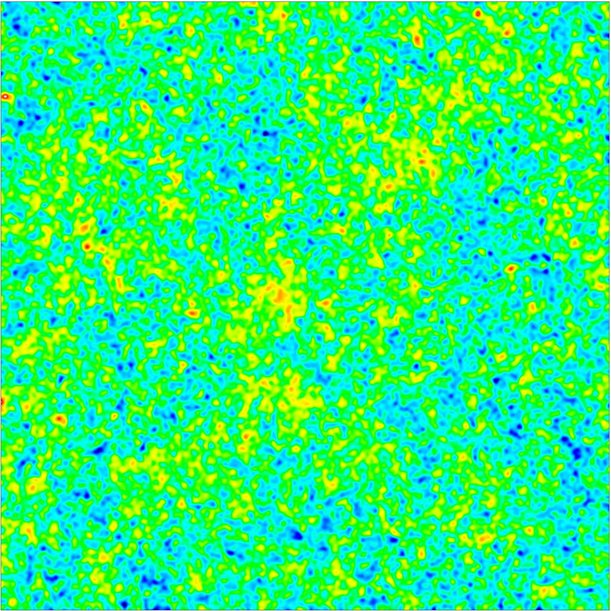
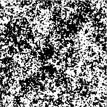
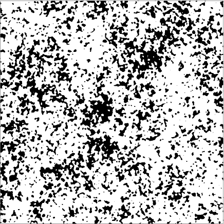
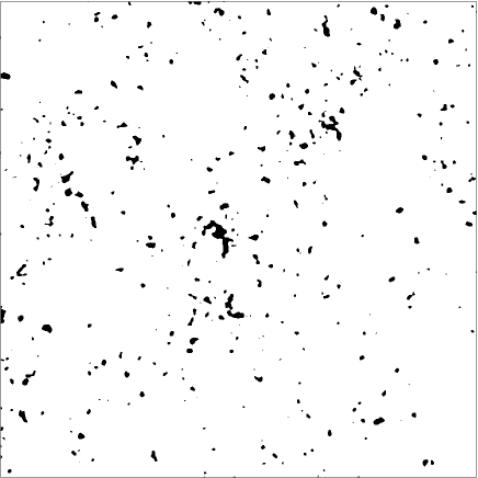
For illustrative purposes, Figure 1 shows one of our 12-square-degree convergence maps in the top left panel, and the excursion set (shown as the black regions) in the other three panels for the three different thresholds $\kappa=0.0,0.02$ and $0.07$. The left column of Figure 2 further shows the mean MFs in each of the 7 cosmological models studied in this paper, averaged over all 1,000 maps in each case ($V_{0}$, $V_{1}$, and $V_{2}$; top to bottom). The right column shows the difference between the mean MF in the fiducial cosmology and the corresponding MF in each of the other cosmologies. The error bars in all panels denote the standard deviation among the 12-square-degree maps in the fiducial model (they are similar in the other cosmologies and are omitted for clarity).

Figure 1: Top left panel: example of a simulated 12-square-degree convergence map in the fiducial cosmology, with intrinsic ellipticity noise from source galaxies and $\theta_{G}=1$ arcmin Gaussian smoothing. A source galaxy density of $n_{gal}=15$/arcmin² at redshift $z_{s}=2$ was assumed. Other three panels: the excursion sets above three different convergence thresholds $\kappa$, i.e. all pixels with values above (below) the threshold are black (white). The threshold values are $\kappa=0.0$ (top right), $\kappa=0.02$ (bottom left), and $\kappa=0.07$ (bottom right). The Minkowski Functionals $V_{0}$, $V_{1}$, and $V_{2}$ measure the area, boundary length, and Euler characteristic (or genus), respectively, of the black regions as a function of threshold.

Figure 2: Left column: the three Minkowski Functionals in two dimensions, $V_{0}$ (area), $V_{1}$ (boundary length), and $V_{2}$ (Euler characteristic) as a function of threshold $\kappa$ derived from 12-square-degree convergence maps in different cosmologies. Right column: differences of MFs in various cosmologies, compared to the fiducial model: control (“auxiliary”) map set in the fiducial model itself, with different realization of initial conditions (black), $\Omega_{m}=0.23$ (red), $\Omega_{m}=0.29$ (pink), $w=-0.8$ (blue), $w=-1.2$ (turquoise), $\sigma_{8}=0.75$ (green), and $\sigma_{8}=0.85$ (yellow). The black error bars show the standard deviation of the MFs among the 1,000 maps of the fiducial map set. A source galaxy density of $n_{gal}=15$/arcmin² at redshift $z_{s}=2$ was assumed and $\theta_{G}=1$ arcmin Gaussian smoothing was applied.

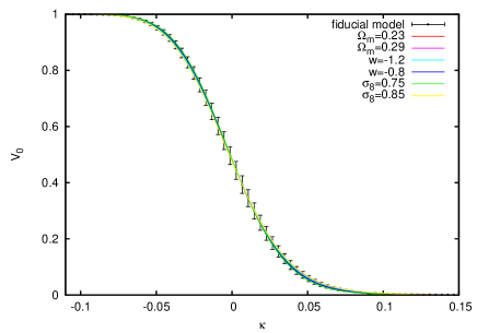
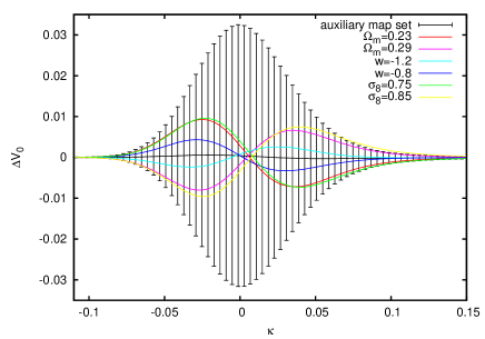
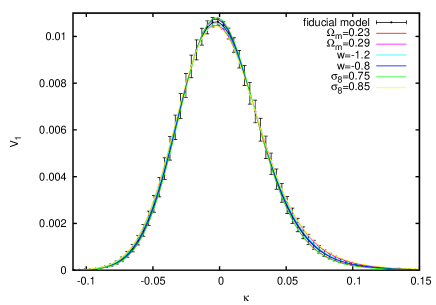
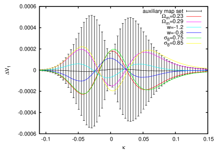
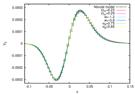
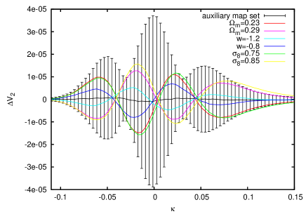
Since MFs are statistics on smoothed fields, while our convergence maps are pixelized, one might worry that a discretized implementation of Eqs. (8)–(10) can lead to spurious “residuals” as seen by some earlier work on MF (see for example Refs. Hikage:2006fe ; Hikage:2008gy ; Matsubara:2010te ). It turns out the residuals are in fact not caused by pixelization, but instead by the discretization of the thresholds, i.e. finite bin-sizes, as first pointed out by Ref. Lim:2011kd . These errors scale like $(\delta\nu)^{2}/\sigma_{0}$ which can be analytically calculated and subtracted if the underlying distribution is known. On the other hand, if we do not know the underlying map, we can work around this problem by using small bin-sizes. While a small bin size means that each bin is more noisy as there are less pixels binned, there are more bins hence once integrated over the amount of information remains the same.

To check for this, we generated 200 $2048\times 2048$ pixelized maps of Gaussian random fields (GRF), and numerically calculated the MFs. In the GRF case, the expectation values for the MFs can be calculated analytically Matsubara:2003yt ,

$$V_{0}^{\mathrm{GRF}}(\nu)=\frac{1}{2}\left[1-\mathrm{erf}\left(\frac{\nu-\mu}{\sqrt{2}\sigma_{0}}\right)\right],$$ (11)

$$V_{1}^{\mathrm{GRF}}(\nu)=\frac{1}{8\sqrt{2}}\frac{\sigma_{1}}{\sigma_{0}}\exp\left(-\frac{(\nu-\mu)^{2}}{2\sigma_{0}^{2}}\right),$$ (12)

and

$$V_{2}^{\mathrm{GRF}}(\nu)=\frac{\nu-\mu}{4\sqrt{2}}\frac{\sigma_{1}^{2}}{\sigma_{0}^{3}}\exp\left(-\frac{(\nu-\mu)^{2}}{2\sigma_{0}^{2}}\right),$$ (13)

where $\mu=\langle\kappa\rangle$ is the mean,

$$\sigma_{0}=\sqrt{\langle\kappa^{2}\rangle-\mu^{2}}$$ (14)

is the standard deviation, and

$$\sigma_{1}=\sqrt{\langle\kappa_{x}^{2}+\kappa_{y}^{2}\rangle}$$ (15)

is its first moment.

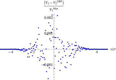
We average the MFs measured from these 200 GRF maps, each with 200 threshold bins from $\nu/\sigma_{0}=-5$ to $\nu/\sigma_{0}=5$, to find the mean $\langle V_{j}\rangle$, and then compare it to the analytic expressions given by Eqns. (11)-(13). In the latter, we use the values $\langle\mu\rangle$, $\langle\sigma_{0}\rangle$ and $\langle\sigma_{1}\rangle$ obtained by averaging over the same 200 maps. As can be seen from Fig. (3), which shows the difference between our numerically calculated and theoretically expected MFs, our procedure reproduces the MFs in the GRF case highly accurately.

Figure 3: Comparison between the average MFs numerically calculated from 200 mock Gaussian random field maps with unit variance, and the analytic expectations given by Eqns. (11)–(13). The x axis shows the value of the threshold, and the y axis shows the fractional differences in the MFs normalized to the maximum value of the respective MF, as labeled.

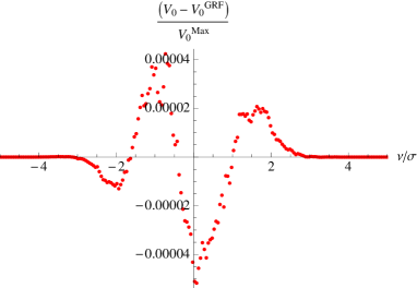
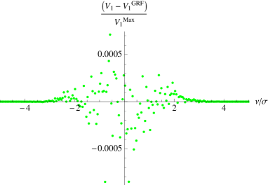
It is instructive to briefly comment on what the MFs measure in broader, qualitative terms. The properties of random fields can be roughly divided into four distinct categories: (a) the histogram, which probes the distribution of pixel values, but is insensitive to their spatial distribution, (b) spatial correlations, which depend on the distances between pixel values, but not about the shapes of structures that lie in between, (c) the shape of objects, and (d) topology, which cares about the connectedness of objects, but by itself is insensitive to their distances or shapes, as it is independent of the underlying metric.

The power spectrum is a pure measure of (b), while the MFs are also sensitive to (a), (c) and (d). In fact, $V_{0}$, the cumulative probability distribution function (PDF), is a pure measure of (a). $V_{2}$, the Euler characteristic of the excursion set, measures the topology (d). However, $V_{2}$ is not a pure measure of connectedness of structures, as it is “contaminated” by the histogram. Intuitively, $V_{1}$ also contains information on (c). This broad classification of information will be useful when interpreting the origin of the constraints from the MFs for different smoothing scales.

III.2 Power Spectra

In order to study the non-Gaussian information content of the MFs explicitly, we also compute the power spectrum from our convergence maps. The power spectra were first pre–computed for 1000 equally spaced bins of the angular wave vector $\vec{\ell}$ between $100\leq|\vec{\ell}|\leq 100,000$, covering the full range of angles from our pixel size ($\sim 6$ arc-sec) to the linear size of our maps ($\sim 3.5$ deg). We further adopted the flat sky approximation, assumed spatial isotropy, and averaged modes with the same length of the wave vector $\vec{\ell}$ in different directions, to find the 1D power spectrum $P(\ell)$ as a function of $\ell=|\vec{\ell}|$ alone.

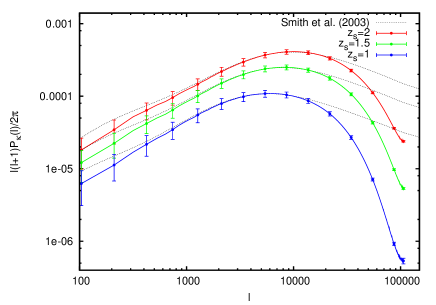
The power spectrum can be derived using the Limber approximation Limber and integrating the 3D matter power spectrum along the line of sight. To check the accuracy of our simulations, ray-tracing code, and construction of the lensing maps, we compare our numerically measured lensing power spectra to the fitting formulae in Smith . For this comparison, we derived power spectra from raw 12-square-degree WL maps (without adding noise or smoothing), and averaged over the 1,000 maps in our fiducial model. The results are shown by the solid curves in Figure 4 for the three different redshifts $z_{s}=1,1.5$, and $2$, with error bars showing the standard deviation of the power in each $\ell$-bin. The dashed curves show the expectations from Smith , which we computed with the public code Nicaea Nicaea .

The figure shows that our simulations lose power below $\ell\sim 400$, due to our finite box size. On smaller scales, we find excellent agreement out to $\ell\sim 20,000$ for $z_{s}=1$ and out to $\ell\sim 30,000$ for $z_{s}=1,5$ and $2$, corresponding to our resolution limit. Because of this limitation, we will employ smoothing scales no smaller than 1 arcmin below. Comparing Figure 4 to Figure 3 in Kratochvil:2009wh , we notice that the drop-off in power has been pushed out to higher $\ell$, due to the increased resolution of the density planes.

Figure 4: Convergence power spectra in the fiducial model from our simulations, for source galaxies at redshift $z_{s}=1,1.5$, and $2$ (from bottom to top, in blue, green, and red, respectively) compared to theoretical predictions calculated with Nicaea Nicaea (black dashed curves). The simulated spectra have been averaged over 1,000 maps, without ellipticity noise or smoothing, and the error bars show the r.m.s. variation among these maps. Power is missing on large scales due to the finite box size of the simulations, and on small scales due to mass resolution and resolution on the $4096^{2}$-pixel density planes.

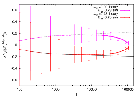
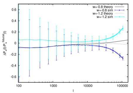
Our results rely mostly on the cosmology-dependence of the power spectrum (and MFs), rather than its absolute value. We therefore compare the differences of the power spectra in various cosmologies from the fiducial case. The results are shown in Figure 5, which shows that the agreement is excellent for the dependence of the power spectrum on all three parameters, down to scales of $\ell\sim 20,000$. The theoretical predictions for the underlying non-linear matter power are good only to about $\sim$10% on scales down to $\sim 0.1$Mpc CoyoteI , which can cause an under-prediction for the convergence power spectrum as well Hilbert:2008kb ; Sato:2009 ; Eifler:2010kt ; the differences are therefore within the accuracy of the theory down to these $\ell$.

Figure 5: Convergence power spectra derived from our simulations are compared to theoretical predictions, as in Figure 4, except we only show results for source galaxies at redshift $z_{s}=2$, and show the differences between the power spectra in various cosmologies compared to the fiducial model.

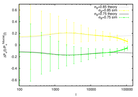
IV Statistical Methods of Analysis

IV.1 Statistical Descriptors

Together, we generically refer to the MFs and the power spectra as statistical “descriptors” of the convergence map. The descriptors can be combined into a single vector, $N_{i}$, where $i$ indexes the threshold for MFs and the multipole for the the power spectrum. Combining the data from several source redshifts or smoothing scales simply makes the descriptor vector longer, but we still treat it in the same way. For each MF, we divide the range into 15 threshold bins. Similarly, we divide the power spectrum into 15 scale bins (we require such a small number to keep the covariance matrix tractable, as discussed below). The most comprehensive case we consider uses three source redshifts, each with five smoothing scales for each of the three MFs, plus the power spectrum, for a total of $15\times 3\times 5\times 4=900$ entries in the $N_{i}$ vector.

To constrain cosmology, we are interested in the true ensemble average (denoted henceforth by brackets $\langle\ \rangle$) and covariance of these descriptors as a function of cosmological parameters ($\mathbf{p}=\{\Omega_{m},w,\sigma_{8}\}$). These of course are not available to us, but can be estimated from the simulations. Averaging over the pseudo-independent map realizations within a given cosmology, we can estimate the ensemble average by

$$\langle{N}_{i}(\mathbf{p})\rangle\approx\overline{N}_{i}(\mathbf{p})\equiv\frac{1}{R}\sum_{r=1}^{R}N_{i}(r,\mathbf{p}),$$ (16)

where $N_{i}(r,\mathbf{p})$ is the descriptor vector for a single realization and $r$ runs over our $R=1000$ map realizations. We call this estimate the simulation mean. It differs from the true ensemble average both because of the limited number of realizations and also because of the limitations inherent in our simulations. In the absence of a fitting formula for the MFs in the non-Gaussian case (analogous to the power spectrum formula from Smith ) the simulation mean serves as our proxy for theoretically predicted MFs. 

Because of the computational expense, we can only form this estimate at our few selected cosmologies (Table 1). Using finite differences between the simulated cosmologies, we construct a first-order Taylor expansion around our fiducial cosmology to estimate $\overline{N}_{i}(\mathbf{p})$ for other cosmologies not explicitly covered by simulations:

$$\overline{N}_{i}(\mathbf{p})\approx\overline{N}_{i}(\mathbf{p_{0}})+\sum_{\alpha}\frac{\overline{N}_{i}(\mathbf{p}^{(\alpha)})-\overline{N}_{i}(\mathbf{p_{0}})}{p^{(\alpha)}_{\alpha}-p_{\mathbf{0}\alpha}}\cdot(p_{\alpha}-p_{\mathbf{0}\alpha}),$$ (17)

Here, index $\alpha=1,2,3$ refers to an individual parameter, such as $\Omega_{m},w$, or $\sigma_{8}$, and the sum counts through all varied cosmological parameters, while $\mathbf{p}^{(\alpha)}$ denotes the cosmological parameter vector of an actually simulated non-fiducial cosmology with only the parameter $p_{\alpha}$ varied. The fraction in Eq. (17) is the finite difference derivative. If the non-fiducial cosmology is chosen such that $p^{(\alpha)}_{\alpha}-p_{\mathbf{0}\alpha}$ is positive, we call it a “forward derivative”, if it is negative, we call it a “backward derivative”. We use either one or the other derivative to compute parameter constraints to assess the robustness of our results.

Similarly to the simulation mean, we estimate the covariance of the statistical descriptors from the simulations, ${\rm Cov}(N_{i},N_{j})\approx C_{ij}$, where

$$C_{ij}(\mathbf{p})\equiv\frac{1}{R-1}\sum_{r=1}^{R}[N_{i}(r,\mathbf{p})-\overline{N}_{i}(\mathbf{p})][N_{j}(r,\mathbf{p})-\overline{N}_{j}(\mathbf{p})].$$ (18)

This covariance matrix contains contributions both from the sample variance of the true convergence signal and from the random ellipticity noise. When the size of this covariance matrix is large, inaccuracies in its estimate can become challenging, as we explore further below.

IV.2 Parameter Estimation and Constraints

In principle – having numerically evaluated Eqs. (16), (18) and the finite difference derivatives for Eq. (17) from the simulated WL maps – one can use the Fisher matrix formalism to compute parameter constraints. In fact, at least two groups have followed this approach recently for weak lensing simulations with redshift tomography Yang:2011zz ; Seo2011 . In practice, however, the Fisher matrix is a forecasting tool and mis-estimation of the covariance from the (simulated) data makes this procedure unstable as we combine smoothing scales and redshifts. As the descriptor $N_{i}$ surpasses several hundred entries, the marginalized error on parameters $\Delta p_{\alpha}^{\rm marg.}=\sqrt{(F^{-1})_{\alpha\alpha}}$ derived from the Fisher matrix $F$ shows a runaway behavior to smaller errors. (Here again, index $\alpha=1,2,3$ refers to an individual parameter, such as $\Omega_{m},w$, or $\sigma_{8}$.) The explanation for this behavior is straightforward, and relates to the imprecise estimation of the covariance matrix from a small number of independent realizations: When the number is insufficient, outliers will be absent, so covariances will typically be underestimated, resulting in overly optimistic error-bars.

Since we want to combine many descriptors, we need a procedure which is robust and conservative when the covariance is poorly estimated. With these requirements, we chose to use $\chi^{2}$-minimization to fit for parameters, then measure the distribution of parameter fits using an ensemble of Monte Carlo realizations.

For realizations drawn from the fiducial cosmology $\mathbf{p_{0}}$, $\chi^{2}$ is

$$\chi^{2}(r,\mathbf{p})\equiv\sum_{i,j}\,\Delta N_{i}(r,\mathbf{p})\,[{\rm Cov}^{-1}\mathbf{(p_{0})}]_{ij}\,\Delta N_{j}(r,\mathbf{p})$$ (19)

where

$$\Delta N_{i}(r,\mathbf{p})\equiv N_{i}(r,\mathbf{p_{0}})-\langle{N}_{i}(\mathbf{p})\rangle.$$ (20)

For each Monte Carlo realization, we minimize $\chi^{2}$ with respect to $\mathbf{p}$ using a simulated annealing algorithm. In practice, the simulation-based estimates described above replace the ensemble average and covariance. Note that we fix the covariance matrix to our estimate at the fiducial cosmology, $C_{ij}(\mathbf{p_{0}})$, but below argue that, for this procedure, having the exact covariance matrix is not crucial. The covariance matrix is inverted with singular value decomposition and condition number $10^{6}$, discarding any problematic eigenvectors. The simulation means, finite differences between cosmologies, and the covariance matrices are all computed with the auxiliary data set (5 N-body simulations), which has the same cosmology as the fiducial data set, but shares random seeds, and therefore large-scale structures, with the realizations from the alternative cosmology simulations. In this way we probe more directly the effect of cosmological differences on these statistical descriptors. It is also important that the covariance matrix is constructed from a map set that is strictly independent of the maps for which $\chi^{2}$ is being evaluated, lest the covariance be erroneously “tuned” to the specific data set.

The maps built from the much larger fiducial data set (45 N-body simulations) make up our Monte Carlo ensemble. The $N_{i}$ vectors computed from these maps are our best representation of the distribution of measured descriptors. The distribution of the parameters fit to these descriptors is used to compute the error bars and confidence contours below. Marginalized errors are computed from the variance of each parameter. To illustrate covariances, we plot approximate two-dimensional error ellipses by computing the covariance between parameters (evaluated over the Monte Carlo ensemble), drawing the 68.4% confidence limit from a corresponding bivariate Gaussian distribution with the same covariance. We checked these contours against the Fisher matrix contours in a few cases, finding good agreement when the covariance matrix is small.

For a large numbers of bins, the Monte Carlo confidence limits are stable, and do not show the runaway behavior we saw for the Fisher matrix estimates. Furthermore, the parameter fits are not strongly biased by a bad choice of covariance matrix (if the system were linear there would be zero bias) although the resulting error bars are not optimal. This means that errors in the estimate of the covariance matrix tend to make our estimate more conservative. Finally, we introduce the notation

$$\chi^{2}_{\rm min}(r)\equiv\min_{\mathbf{p}}\chi^{2}(r,\mathbf{p})$$ (21)

for the minimized $\chi^{2}$ for map $r$, and $\chi^{2}_{\rm min}/n$ for the $\chi^{2}$ per degree of freedom in this best-fit model. Here the number of degrees of freedom is the length of $N_{i}$ minus the three model parameters varied. Averaged over realizations, $\overline{\chi}_{\rm min}^{2}/n$ is an indicator for the typical goodness of fit (and in the case of Gaussian errors, would be $\lesssim 1$). On the other hand, errors in the covariance estimate will make the fit worse, so we use this quantity as a diagnostic of the quality of the estimate.

IV.3 Binning

Here we give more details on our choices of binning. We pre-compute the MFs for 200 equally spaced convergence thresholds $\kappa$ and the power spectrum for 1,000 equally spaced values of $\ell$. Before the analysis, we divide the MFs into 15 equally spaced bins in $\kappa$. To avoid bins lying in noisy regions where outliers in a few maps dominate (i.e. very high and low thresholds $\kappa$), we restrict ourselves to the range where the simulation mean of the MFs is at least 5% of its maximum value. In the case of $V_{0}$, we use the differential (instead of the standard cumulative) version of the MF to determine the $\kappa$ range.

The power spectrum is originally computed in narrow, equally spaced bins, which we rebin into 15 logarithmic bins (based on the bin minimum), as close to logarithmic as possible without interpolation. The logarithmic bins span $\ell=100$–$20,000$, from the largest mode in the map to our smallest smoothing scale $\theta_{G}=1$ arcmin. Using upper cutoffs at $\ell=40,000$ and $\ell=80,000$ does not change the results appreciably.

IV.4 Breakdown of the Covariance Matrix Estimate

The size of our covariance matrix varies from $15\times 15$ elements for a single descriptor, redshift, and smoothing scale to $900\times 900$ elements for all three MFs combined with the power spectrum, redshift tomography with three source galaxy planes, and five smoothing scales all combined. Unless all descriptors are highly correlated, it is clearly very difficult to estimate all elements accurately from merely $R=1000$ maps. We therefore expect that as we increase the number of threshold or multipole bins, combine more descriptors, redshifts, or smoothing scales, at some point, our results become unreliable just because we have too few maps.

When we compute the marginalized errors both from the Fisher matrix and from the Monte Carlo procedure, as mentioned above, they agree for small $N_{i}$ vectors. Ideally, as the vector’s number of entries is increased beyond the point where no more information can be gleaned from the fine shape of the MFs or the power spectrum, the errors computed from the Fisher matrix and from the Monte Carlo method would both reach a plateau. In practice, as one increases the number of entries further beyond the quality limit of the dataset, the marginalized errors from the Fisher matrix start improving further as long as one keeps adding bins, even if there is no new information content in them. This is clearly unphysical (and comes from underestimating the [co]variances, as pointed out above). In contrast, we find that the Monte Carlo errors start increasing modestly in such a situation. This behavior of the Monte Carlo results is also unphysical—the constraints on parameters cannot become worse when no or more information is added.

The difference between the behavior of the Fisher matrix and the Monte Carlo is crucial when applying these techniques to simulation data, as opposed to doing forecasting from a predictive analytic theory. In particular, the derived constraints become unreliable if the quality of the dataset is insufficient (or just barely sufficient) to reach the plateau, i.e. the covariance matrix gets corrupted before (or just as) the best constraints are reached. Then no plateau can be identified and the Fisher matrix constraints keep continuously improving – most importantly, there is no indication of when one transitions into the unphysical breakdown regime. The Monte Carlo method, on the other hand, provides a conservative estimate in this case: as long as the quality of the data allows it, the parameter constraints will improve, and when the quality limit of the data is reached—not because there is no more information in principle, but because there is insufficient data to give good enough estimates for the covariance matrix—the constraints start to worsen again modestly. In that case one can simply take the tightest Monte Carlo constraints achievable to get the best constraints which the given dataset allows. In our cases with multiple descriptors, redshifts, and many smoothing scales, we have found it difficult to get a good enough dataset to see a plateau.

In addition to seeing the constraints degrade, the minimum value of $\chi^{2}$ can indicate when this breakdown occurs. Empirically, we note that as the confidence contours reach their achievable minimum from our data, the $\overline{\chi}^{2}_{\rm min}/n$ starts to rise, eventually reaching $\overline{\chi}^{2}_{\rm min}/n\approx 2$ which signals the beginning of the unphysical breakdown. For example, when all three MFs are combined, with all three redshifts and all five smoothing scales, we have 675 entries in $N_{i}$ and $\overline{\chi}^{2}_{\rm min}/n\approx 1.9$, at which point the contours become a few percent larger than for just three smoothing scales. Further adding the power spectrum to these constraints results in 900 entries and $\overline{\chi}^{2}_{\rm min}/n\approx 2.8$, and the contours begin to widen noticeably. We therefore take this limit as the breakdown of our simulated map set.

This behavior, which is the opposite of the Fisher matrix approach that tends to underestimate the errors, makes our Monte Carlo results conservative with respect to inaccuracies in the covariance matrix.

V Results

Utilizing the Monte Carlo procedure, we were able to obtain reliable constraints for combinations of three source redshifts $z_{s}=1,1.5,2$ and five smoothing scales $\theta_{G}=1^{\prime},2^{\prime},3^{\prime},5^{\prime},10^{\prime}$ for nearly all combinations of the MFs and power spectra.

Figure 6 shows two-dimensional confidence contours, in each case marginalized over the third parameter, from the three individual MFs $V_{0}$ (blue), $V_{1}$ (green), and $V_{2}$ (red), from all three MFs combined (pink), as well as from the power spectrum alone (turquoise). The lower panels also show the MFs with the power spectrum combined (black). The ellipses shown in this figure enclose 68.4% of the likelihood, as calculated from the covariance of the best-fit parameter values with our Monte Carlo procedure described in Section IV.2. Table 2 shows the corresponding 68.4% confidence limits on individual parameters, marginalized over the other two parameters.

The table and the figure are both scaled from the simulated 12-square-degree maps to the 20,000-square-degree solid angle of a full-sky survey, such as LSST (i.e. by a factor of $\sqrt{12/20,000}\approx 1/40$). All results shown in this section were computed using the backward finite difference derivative in (17), which in our cases yielded slightly wider constraints than the forward derivative. We explore the difference between the two derivative types explicitly in Sec. V.7.

	$\Delta\Omega_{m}$	$\Delta w$	$\Delta\sigma_{8}$
$z_{s}=2$; $\theta_{G}=1^{\prime}$
$V_{0}$	0.00317	0.0152	0.00393
$V_{1}$	0.00191	0.0111	0.00263
$V_{2}$	0.00187	0.0118	0.00262
PS	0.00297	0.0193	0.00478
MFs	0.00175	0.00979	0.00237
$z_{s}=2$; $\theta_{G}=1^{\prime},2^{\prime},3^{\prime},5^{\prime},10^{\prime}$
$V_{0}$	0.00153	0.00846	0.00215
$V_{1}$	0.00163	0.0087	0.00226
$V_{2}$	0.00158	0.00931	0.00228
PS	0.00288	0.0189	0.00475
MFs	0.00121	0.00668	0.00183
$z_{s}=1,1.5,2$; $\theta_{G}=1^{\prime}$
$V_{0}$	0.00174	0.011	0.00204
$V_{1}$	0.00141	0.00982	0.00188
$V_{2}$	0.00135	0.00998	0.00183
PS	0.00156	0.0159	0.00206
MFs	0.00122	0.00846	0.00174
$z_{s}=1,1.5,2$
$\theta_{G}=1^{\prime},2^{\prime},3^{\prime},5^{\prime},10^{\prime}$
$V_{0}$	0.000958	0.0064	0.00143
$V_{1}$	0.000916	0.00634	0.00131
$V_{2}$	0.00095	0.00642	0.0014
PS	0.0015	0.0151	0.00206
MFs	0.000912	0.00552	0.00144

Table 2: 68.4% confidence limits on cosmological parameters from the three Minkowski Functionals and from the power spectrum, marginalized over the other two varied parameters—with and without combining smoothing scales and with and without using tomography, as indicated in the table. Intrinsic ellipticity noise from source galaxies with a surface density of $n_{gal}=15$/arcmin² on each redshift plane has been included. The numbers have been scaled from our 12-square-degree maps to a full-sky LSST-like survey.

Without Redshift Tomography:


With Redshift Tomography:

Figure 6: Comparison of constraints from the Minkowski Functionals ($V_{i}$) and the convergence power spectrum, scaled to a full sky survey with a source galaxy density of $n_{gal}=15$/arcmin² per source redshift plane. The colors denote: $V_{0}$ (blue), $V_{1}$ (green), $V_{2}$ (red), $V_{0}$, $V_{1}$, and $V_{2}$ combined (pink), power spectrum (turquoise), and—only in the lower panels—MFs combined with the power spectrum (black). The ellipses depict 68.4% confidence contours, marginalized over the third parameter not shown in each panel. The top two rows show the constraints from a single redshift $z_{s}=2$, with either a single smoothing scale $\theta_{G}=1^{\prime}$ (first row) or all five smoothing scales $\theta_{G}=1^{\prime},2^{\prime},3^{\prime},5^{\prime},10^{\prime}$ combined (second row). The lower set of two rows show the same, except using redshift tomography with $z_{s}=1,1.5$ and $2$ combined. Only three smoothing scales $\theta_{G}=1^{\prime},3^{\prime},10^{\prime}$ were combined in the lowest row to improve numerical stability. The MFs constrain all cosmological parameters more tightly than the power spectrum alone, especially the dark energy equation of state parameter $w$ (by a factor of $\sim$two). Combining smoothing scales tightens the MF constraints much more significantly than those from the power spectrum; tomography helps to further tighten constraints.

Figure 6 has four rows. In each row, the 3 panels show the 3 projections of the likelihood ellipsoid in the $\Omega_{m},w,\sigma_{8}$ space. The top two rows show the constraints from a single redshift $z_{s}=2$, with either a single smoothing scale $\theta_{G}=1^{\prime}$ (first row) or all five smoothing scales $\theta_{G}=1^{\prime},2^{\prime},3^{\prime},5^{\prime},10^{\prime}$ combined (second row). The lower set of two rows show the same, except using redshift tomography with $z_{s}=1,1.5$ and $2$ combined. We use only three smoothing scales $\theta_{G}=1^{\prime},3^{\prime},10^{\prime}$ for the last row of the figure, because for the power spectrum it does not make any difference and for the combined MFs it gives slightly tighter constraints by a few percent for the numerical reasons described in Sec. IV.4. The individual MFs show very similar constraints to each other and keep the same relative size to the combined-MF contour as in the second row, so we retain them only in Table 2 for the redshift tomography case. For the individual MFs, the constraints are tightest with all smoothing scales combined, even in the case of redshift tomography. We will comment on the black ellipse in the third and fourth row of Figure 6 in Sec. V.4.

These are the main results of this paper, and we next turn to interpreting them further.

V.1 Information Beyond the Power Spectrum

A comparison of the pink ellipse (MFs combined) with the turquoise (power spectrum) in Figure 6 shows that the MFs constrain all three parameters $\Omega_{m}$, $w$, and $\sigma_{8}$ more tightly than the power spectrum. The tightest constraints are obtained when all five smoothing scales are combined and redshift tomography is included (the bottom row in the figure). The “MFs” and “PS” rows in Table 2 demonstrate the same result for the marginalized errors on the individual parameters. While $\Omega_{m}$ and $\sigma_{8}$ are constrained by the MFs only modestly better, there is a much more significant improvement on the $w$ constraint, by a factor of $\approx$three. Therefore, the MFs appear particularly useful to improve constrains on dark energy.

We would next like to understand the origin of these constraints better. Looking at the leftmost panel of the first row in Figure 6, we see that the power spectrum has a degeneracy in the $(w,\sigma_{8})$–direction. This degeneracy appears consistent from the changes in the power spectra in panel 2 in Figure 5, which shows that for $\sigma_{8}$ fixed, the overall normalization of the power spectrum is a bit lower for the $w=-0.8$ model than for the fiducial cosmology, and therefore $\sigma_{8}$ in the $w=-0.8$ model would need to be increased slightly to make it look more like the fiducial model power spectrum. This explanation, however, ignores the fact that in Figure 6 a third parameter is varied, $\Omega_{m}$. Further, we note that in addition to the overall growth, geometrical distance factors contribute importantly to the overall $w$-sensitivity of the convergence power spectrum, e.g. Zhan2009 .

Interestingly, the MFs show an even stronger degeneracy in the $(w,\sigma_{8})$ plane, but in a nearly orthogonal direction. All three MFs place tights constraints in the direction of the degeneracy of the power spectrum, even without tomography or combining multiple smoothing scales. It is instructive to further examine the behavior of the constraints from $V_{0}$, with and without combining smoothing scales. As mentioned above, in the case of a single smoothing scale, $V_{0}$ is equivalent to the fractional area statistic (or histogram), but when multiple scales are combined, $V_{0}$ receives, additionally, spatial information. We see that combining several smoothing scales tightens the $V_{0}$ constraints only modestly in the $(w,\sigma_{8})$–correlation direction, but results in a significant improvement in the orthogonal, $(w,\sigma_{8})$–anticorrelation direction. We conclude that in this $(w,\sigma_{8})$–anticorrelation direction, the non-Gaussian information in the maps is coming from beyond the histogram, whereas in the direction of $(w,\sigma_{8})$–correlation, most of the information is already contained in the histogram. This suggests that most of the value of the MFs, which helps break degeneracies of $w$ with other parameters in the power spectrum, is contained in $V_{0}$, and the single smoothing scale $\sim 1$arcmin is sufficient to get most of the benefits. We elaborate on this finding further in Section V.3 below.

V.2 Redshift Tomography

As is well–known, varying either $\Omega_{m}$ or $w$ changes both the expansion history of the universe and the redshift dependence of the amplitude of the power spectrum. In contrast, $\sigma_{8}$ changes only the overall normalization of the power spectrum, without modifying its redshift evolution (at least in the linear regime). For a single redshift, the amplitude of the matter fluctuations $\sigma_{8}$ can be tuned to compensate for the changes in $\Omega_{m}$ or $w$, but this degeneracy is broken when several redshifts are considered simultaneously.

As Table 2 shows, redshift tomography is especially useful to break the $(\Omega_{m},\sigma_{8})$–degeneracy in the constraints from the power spectrum, improving constraints on $\Omega_{m}$ and $\sigma_{8}$ by factors of 2–3. The tomographic improvements for $w$, and on all three parameters from the MFs, are somewhat more modest ($\sim 20-30$%). Tomography affects the constraints somewhat more weakly for the MFs, in part because the $(\Omega_{m},\sigma_{8})$–degeneracy is weaker to begin with. Interestingly, Fig. 6 shows further that in the $(w,\sigma_{8})$ plane, tomography tightens the power spectrum constraints almost entirely in the $\sigma_{8}$ direction, leaving the constraint on $w$ relatively unimproved. This is why, in comparison, the MFs provide a factor of $\sim$three better marginalized constraint on $w$, even after redshift-tomography is included.

V.3 Combining Smoothing Scales

Combining smoothing scales turns out to be crucial for MFs – even more important than tomography. This was already anticipated in whm09 , and is here clearly evidenced by the tighter constraints in the 2nd and 4th row in Figure 6, where multiple smoothing scales are combined. This is in sharp contrast with the power spectrum, where combining smoothing scales results in negligible improvements (as it should, at least in the linear regime). The improvements are most pronounced in the constraints from $V_{0}$, especially for a single redshift, as can be seen by comparing the upper left panel with the left panel in the second row. We thus further examine this case, as an example of how MFs derive information from smoothing scale combinations.

Consider the $(w,\sigma_{8})$–anticorrelation direction in the top left panel of Figure 6. As we have noted above, the power spectrum constraints are strongest in this direction. The power spectrum measures spatial correlations, and $V_{0}$ is completely blind to spatial arrangements of pixel values, when only a single smoothing scale is used. It is therefore unsurprising to see that $V_{0}$ constraints in this direction are particularly weak. The other two MFs – both sensitive to aspects of shape and topology – incorporate some spatial information, and fare much better. However, when we combine multiple smoothing scales, the $V_{0}$ constraint tightens to the same level as the other MFs (see left panel in the second row). This makes intuitive sense, since combining smoothing scales adds spatial distribution information to $V_{0}$: Whether peaks on smaller scales are clustered together determines if they survive large-scale smoothing or get washed out by it.

The above interpretation can be further illuminated by considering the theoretical predictions for the MFs for GRFs. We see from Eqs. (14)–(15) that $V_{0}$ depends only on $\sigma_{0}$, defined in Eq. (14). This is a simple integral of the power spectrum, and is insufficient to capture all the cosmological information in the $(w,\sigma_{8})$–anticorrelation direction. In comparison, $V_{1}$ and $V_{2}$ depend, additionally, on $\sigma_{1}$, the first moment of the power spectrum defined in Eq. (15), which weighs high $\ell$ more than $\sigma_{0}$. In combination, these two integrals provide additional cosmological information from the shape of the power spectrum. When combining different smoothing scales, the power spectrum is truncated at different values of $\ell$. As a result, the combination of $\sigma_{0}$’s from different smoothing scales captures information from the $\ell$–dependence of the power spectrum, providing $V_{0}$ with information that is similar to $V_{1}$ and $V_{2}$.

This raises the question: How many smoothing scales does one need? Combining too many smoothing scales increases the size of the covariance matrix and can render the results unreliable, as discussed above. Table 3 shows the marginalized constraints from different individual smoothing scales and from their combinations for all three MFs combined.

Unsurprisingly, the smallest smoothing scale, $\theta_{G}=1$ arcmin, provides the tightest constraints, and the constraints get progressively weaker for larger smoothing scales, up to a factor of $\sim 2$ for $\theta_{G}=10$ arcmin. Nevertheless, there is complementary information in these larger scales. Interestingly, the table shows that one needs to combine at least three scales to get most of the improvement shown by the combination of all five scales we studied. (Since we have not probed more than five smoothing scales, we cannot say whether adding even more scales may further improve the result.)

	$\Delta\Omega_{m}$	$\Delta w$	$\Delta\sigma_{8}$
$\theta_{G}=1^{\prime}$	0.00175	0.00979	0.00237
$\theta_{G}=2^{\prime}$	0.00199	0.0106	0.00268
$\theta_{G}=3^{\prime}$	0.00201	0.0108	0.00283
$\theta_{G}=5^{\prime}$	0.00225	0.0127	0.00316
$\theta_{G}=10^{\prime}$	0.00322	0.0152	0.00468
$\theta_{G}=1^{\prime},3^{\prime}$	0.00155	0.00849	0.00211
$\theta_{G}=1^{\prime},5^{\prime}$	0.00149	0.00816	0.00212
$\theta_{G}=1^{\prime},2^{\prime},3^{\prime}$	0.00142	0.00757	0.00197
$\theta_{G}=1^{\prime},3^{\prime},10^{\prime}$	0.00139	0.00735	0.00196
$\theta_{G}=1^{\prime},2^{\prime},3^{\prime},5^{\prime},10^{\prime}$	0.00121	0.00668	0.00183

Table 3: Marginalized constraints on cosmological parameters from all three MFs combined, for different individual smoothing scales and from various smoothing–scale combinations. See the caption of Table 2 for a further explanation of the numbers in the table. A single source redshift $z_{s}=2$ was assumed. The table shows that combining smoothing scales is advantageous for MFs and does not reach a minimum for at least five scales.

V.4 MFs combined with Power Spectrum

We have so far compared the constraints from MFs with those from the power spectrum. Since the constraints from the MFs is stronger, it is clear that the MFs contain information beyond the power spectrum. However, another interesting question is: To what extent are the constraints from the MFs and the power spectrum independent? Could constraints tighten further when they are combined?

To answer this question, ideally we would like to combine the MFs with the power spectrum, using all five smoothing scales, as well as redshift tomography. Unfortunately, as discussed above, the covariance matrix in this case exceeds the maximum reliable size allowed by our simulated datasets.

However, we have found that combining only three smoothing scales, the results remain stable (in the sense discussed in §IV.4 above) even when tomography with all three redshifts $z_{s}=1,1.5,2$ is used. Table 4 and the last row of Figure 6 show the results in this case. The figure shows the projected error ellipses from the power spectrum only (turquoise), from all three MFs combined (pink), and from the combination of all three MFs and the power spectrum (black); the table shows the corresponding marginalized constraints on the individual parameters. Clearly, adding the power spectrum does not yield any improvement on the constraints already available from the MFs.

Since we are operating at the quality limit of our dataset, we evaluated several other combinations with smaller covariance matrices. The third row of Figure 6 shows redshift tomography with only one smoothing scale. At first glance, here adding the power spectrum to the MFs seems to show a small advantage: The contours get 11% tighter for $\Omega_{m}$ and 14% tighter for $w$ and $\sigma_{8}$. However, this is because only a single smoothing scale is used, which does not extract the maximum amount of information from the MFs. If one studies only one redshift and combines all five smoothing scales, again nothing is gained from adding the power spectrum to the MFs.

This paints a complete picture. We conclude that as long as several smoothing scales are combined, the MFs already extract all the information which is in the power spectrum.

	$\Delta\Omega_{m}$	$\Delta w$	$\Delta\sigma_{8}$
PS	0.00147	0.0151	0.00209
MFs	0.000858	0.00549	0.00126
MFs+PS	0.000815	0.00553	0.0012

Table 4: Marginalized constraints on cosmological parameters from the power spectrum, the three Minkowski functionals (MFs) combined, and from the power spectrum together with the MFs. Redshift tomography with source planes at $z_{s}=1,1.5,2$ and a combination of three smoothing scales $\theta_{G}=1^{\prime},3^{\prime},10^{\prime}$ were used (using all five smoothing scales with tomography would have caused the constraints to widen by a few percent for numerical reasons, see text). Intrinsic ellipticity noise from a source galaxy surface density of $n_{gal}=15$/arcmin² per redshift plane has been included. The table shows that the MFs already include all of the information that is in the power spectrum: Adding the power spectrum does not improve the constraints further. These are our tightest constraints.

V.5 Noiseless Minkowski Functionals

To illustrate the effect of ellipticity noise on our constraints, we repeated our analysis on noiseless maps, for all three redshifts $z_{s}=1,1.5,2$ and three smoothing scales $\theta_{G}=1^{\prime},3^{\prime},10^{\prime}$ combined, which constitutes our best numerically still stable case. For reference, we note that the r.m.s. fluctuations in $\kappa$ caused by large-scale structures at $z_{s}=2$ are $\sigma_{\kappa}=0.022$, very close to the r.m.s. noise $\sigma_{\rm noise}=0.023$ added to the maps Yang:2011zz . We thus expect noise to degrade the constraints by of order a factor of $\sim$two.

The results are displayed in Table 5 and Figure 7. As before, the figure shows the constraints from the power spectrum alone (turquoise), the three MFs combined (pink) and the combination of the MFs and the power spectrum (black).

The table and the figures demonstrate that the constraints are tighter than in the noisy case. We also find that noise hurts the power spectrum somewhat more than the MFs: The degradation due to noise for the marginalized constraint on $\Omega_{m},w$, and $\sigma_{8}$ is a factor of 2.1, 2.8, and 1.8 for the power spectrum (close to the expected factor of $\sim$two), whereas the corresponding degradations for the MFs are factors of 3.4, 3.0, and 3.2. As a result, in the noiseless case, the MFs outperform the power spectrum by a factor of $\sim 3$, larger than in the noisy case.

	$\Delta\Omega_{m}$	$\Delta w$	$\Delta\sigma_{8}$
PS	0.00067	0.00534	0.00105
MFs	0.00025	0.00184	0.000408
MFs+PS	0.00025	0.00183	0.000403

Table 5: Comparison of marginalized constraints from the MFs, the power spectrum, and from their combination, but without adding any intrinsic ellipticity noise. This table is the noiseless equivalent of Table 4.

Figure 7: Comparison of 68.4% confidence ellipses from maps without intrinsic ellipticity noise. This figure is the noiseless equivalent of the last row of Figure 6. The colors are the same as in that figure. The figure shows that noise hurts the MFs more than the power spectrum: the MFs (pink) have a larger advantage—a factor of almost $\approx 3$— over the power spectrum (turquoise) than in the noisy maps. As in the case with noise, adding the power spectrum to the MF constraints (black) yields no further improvement.

V.6 Comparison to Previous Results

To validate our simulation pipeline, as well as our results, we next compare the results of our Fisher matrix analysis for the power spectrum to a recent theoretical study Berge:2009xj . While there are many other previous estimates for cosmological constraints from the WL power spectrum (e.g. Song and Knox (2004), and for a very recent study, examining constraints from power spectrum of the logarithm of the convergence field, see Seo2011 ) the specifications in the study by Berge:2009xj are closest to the present work. In particular, those authors present a two–dimensional Fisher ellipse, in Figure 5 of their paper, in which they vary only the two parameters $\Omega_{m}$ and $\sigma_{8}$ . Their results were computed for a source galaxy redshift distribution around $z_{s}=1$ and surface density of $n_{gal}=40$/arcmin². We have therefore rerun our analysis for the same source galaxy surface density, and plot our power spectrum constraints in Figure 8 for $z_{s}=1$. We have also kept $w$ fixed at its fiducial value of $w=-1$. The solid (dashed) ellipse uses backward (forward) finite differences. The agreement between both the orientation and overall size of our error ellipse and that shown in Figure 5 of Berge:2009xj is very good, especially considering that theirs is for a different cosmology with $(\Omega_{m},\sigma_{8})=(0.3,0.9)$. Ours is a factor of 1.25 larger in $\Omega_{m}$ and a factor of 1.4 in $\sigma_{8}$.

Figure 8: Error ellipse from the convergence power spectrum alone in the ($\Omega_{m},\sigma_{8}$) plane, with $w$ held fixed. This is to be compared to Figure 5 in ref. Berge:2009xj , who use $n_{gal}=40$/arcmin² and a source galaxy redshift distribution around $z_{s}=1$ for a different cosmology $(\Omega_{m},\sigma_{8})=(0.3,0.9)$. To resemble the parameters of Berge:2009xj as closely as possible, we adopted $n_{gal}=40$/arcmin² and $z_{s}=1$, but use our fiducial cosmology. The dashed [solid] contour uses forward [backward] finite difference derivatives. The agreement of our ellipse with Figure 5 in Berge:2009xj is very good, validating our pipeline and results.

V.7 Accuracy

Here we discuss the variability of the error contours under different sets of maps for the fiducial model, to get an estimate of how much our results depend on the particular set of simulations and realizations of individual lensing maps. We then enumerate other possible caveats and systematic errors that we did not explicitly take into account.

V.7.1 Uncertainties Explicitly Evaluated

We have two strictly independent sets of 1,000 maps in the fiducial model, obtained using different sets of N-body runs. We thus have a choice of which of these sets to use for (i) computing the Simulation Mean (eq. 16), and (ii) computing the covariance matrix (eq. 18), and (iii) minimizing $\chi^{2}$ and Monte Carlo. In all of our results so far, we used the auxiliary set for the Simulation Mean and the covariance matrix, and the fiducial set for Monte Carlo. We repeated our calculations by swapping the map sets used for the covariance matrix and for Monte Carlo, and confirmed that this has a negligible effect on our results. Additionally, we have found that for the MFs the results are almost independent of the set used for the Simulation Mean. Although we found a dependence on which set is used for the Simulation Mean for the power spectrum, this is modest: The change is smaller by a factor of 3–4 than the dominant source of variability described in the next paragraph and expresses itself mostly as a slight rotation of the ellipse rather than a change in its size.

The largest numerical variability, however, comes from the difference between the forward vs. backward finite difference used for the parameter dependence of the descriptors in the Taylor expansion (eq. 17), which can be taken as an indication of the robustness of our constraints. Evidently, our choice of parameter spacing between the simulations was somewhat outside the linear regime, such that these two differences yield different derivatives. This is the dominant source of uncertainty. We decided against a higher-order interpolation scheme to improve on our analysis because these variations are modest in most cases, and furthermore, they affect the power spectrum and the MF results in similar ways. Therefore, we have confidence that the relative strength of our constraints between the power spectrum and the MFs holds accurately.

We illustrate the effect of using the two different derivatives on the contours from MFs and the power spectrum in Figure 9 for one redshift $z_{s}=2$ and one smoothing scale $\theta_{G}=1$ arcmin. This figure is the equivalent of the first row in Figure 6, but with both derivative cases shown. The solid and dashed curves in the figure indicate the constraints calculated from backward and forward finite differences in eq. (17) between our simulations, respectively. The differences between the ellipses in the figure are of a representative size: The difference between the contours from the two derivatives tends to get smaller as more redshifts and smoothing scales are combined. In all our other figures and tables we choose to show only the more conservative of the two: results using the backward derivative. The difference in the error contours is still small enough so that it does not affect our overall conclusions. The errors due to the choices of map sets are small in comparison and are not shown.

Without Redshift Tomography:

Figure 9: Illustration of the largest source of variability in our numerical results. In addition to showing the constraints from using the backward finite difference derivatives (solid) in the Taylor expansion Eq. (17) as in the other figures, here we also show the ellipses computed from the forward derivatives (dashed). Otherwise this figure is the same as the first row of Figure 6 for $z_{s}=2$ and $\theta_{G}=1$ arcmin, but showing only the constraints from the MFs combined (pink) and the convergence power spectrum (turquoise). The differences between the ellipses from different derivatives are small enough not to impact our conclusions, and tend to get even smaller as more redshifts and smoothing scales are combined. Furthermore, the relative differences between the MFs and power spectrum are well preserved in both cases individually.

V.7.2 Other Sources of Error

Our study was aimed at a theoretical exploration of the cosmological information content and utility of the MFs. As such, we made a list of idealized assumptions – we here present a partial list of neglected sources of systematic errors, which will have to be quantified in future work.

We used convergence in our maps, rather than the reduced shear that will be available directly from the observations. One can, in principle, convert one quantity to the other; in practice, on small scales, where the MFs derive most of their constraining power, the errors introduced by this conversion will not be negligible, and must be taken into account when extracting cosmological parameters from actual data (e.g. Dodelson:2005ir ).

We assumed the noise from the intrinsic ellipticities of the source galaxies is given by independent Gaussian distributions, with a single width determined by the assumed average source galaxy density. This neglects effects such as shot noise from random galaxy positions, correlations due to intrinsic alignments of galaxies, and magnification bias. In the future, ellipticity noise should be incorporated more accurately, using a mock galaxy catalog with random galaxy positions and intrinsic ellipticity components drawn from more realistic (non-Gaussian) probability distributions, which would then have to be added to the two independent components of the shear signal separately. Additionally, a realistic redshift-distribution of source galaxies should be employed, and photometric redshift errors folded in the analysis, rather than confining all galaxies to fixed redshift planes.

Furthermore, there are systematic effects from the atmosphere and the instrument of a real telescope on one hand, as well as holes in the maps due to foreground stars and other impurities, which we have not taken into account.

The small simulation box size causes a fall–off in the power spectrum on large scales, and we were unable to study correlations between fields larger than 12 square degrees, assuming them to be independent in our idealized full-sky scaling.

Finally, the variance in our MF bins may be somewhat underestimated, because we use only 45 independent N-body simulations to create our pseudo-independent 1000 convergence maps for the fiducial cosmology, and only 5 N-body simulations for the maps of the other cosmologies. We plan to create a larger suite of N-body simulations, and study the importance of the number of independent runs required for weak lensing map generation, in a future paper. On the positive side, a larger suite of runs would allow us to study the dependence of the (co)variances $C_{ij}$ themselves on the background cosmology, and to assess whether these add significant extra information.

VI Conclusions

We have studied the cosmological information content of Minkowski functionals (MF) derived from mock weak lensing maps from an extensive suite of ray-tracing N-body simulations. While there have been a few smaller precursor works, applying MFs to weak lensing maps, this is the first large systematic study to our knowledge. Our N-body simulations cover seven different cosmological models, bracketing the parameters $\Omega_{m}$, $\sigma_{8}$, and $w$ around a fiducial $\Lambda$CDM cosmology. We created convergence maps with ray-tracing, added intrinsic ellipticity noise from the source galaxies, and obtained joint confidence limits on parameters with a Monte Carlo procedure.

Our main result is that there is a substantial amount of information from non-Gaussian features in WL maps, which, as we have explicitly verified, is coming from beyond the power spectrum. In particular, the constraints on the dark energy equation of state parameter, $w$, marginalized over $\Omega_{m}$ and $\sigma_{8}$, is nearly a factor of three tighter than from the power spectrum alone. From combining the MFs with the power spectrum, we also demonstrated that the MFs contain all of the information available from the power spectrum.

The non-Gaussian information extracted by the MFs resides in part in the one-point function of the convergence, which places constraints primarily in the $(w,\sigma_{8})$–correlation direction, and helps break the strongest degeneracy between these parameters present in the power spectrum. When multiple smoothing scales are combined, the MFs derive further information from the morphology and topology of the iso-convergence contours, and place tight constraints in the orthogonal $(w,\sigma_{8})$–anticorrelation direction. We further find that redshift tomography is important to break the degeneracy between $\Omega_{m}$ and $\sigma_{8}$. However, the marginalized constraint on $w$ from the power spectrum alone remains much less affected by tomography.

It would be interesting to study how the constraints from Minkowski functionals complement those from the power spectrum under more realistic survey conditions—with improved theoretical modeling, and including instrument and atmospheric systematics. The MFs will be available automatically in future WL survey data, and our results suggest that they will improve cosmological constraints. Their treatment here is an important step towards realizing the full potential of weak lensing maps, including the information from nonlinear structures.

VII Acknowledgments

We thank Volker Springel for useful discussions and for providing the N-body initial conditions generator N-GenIC, Lam Hui for providing us with a $w$-capable linear growth factor code, and Xiuyuan Yang and Dennis Simon for helpful discussions. We also thank Leonard Slatest and Efstratios Efstathiadis for help with the IBM Blue Gene at BNL.

JMK and KMH acknowledge support from JPL through subcontract 1363745. This research utilized resources at the New York Center for Computational Sciences at Stony Brook University/Brookhaven National Laboratory which is supported by the U.S. Department of Energy under Contract No. DE-AC02-98CH10886 and by the State of New York. Almost all the calculations were performed on the IBM Blue Gene/L and /P New York Blue. The matter power spectra for initial conditions and the $\chi^{2}$–minimization procedure were calculated on the LSST/Astro Linux cluster at BNL.

References

- (1) M. Zaldarriaga, R. Scoccimarro, Astrophys. J. 584, 559-565 (2003).
- (2) F. Bernardeau, L. Van Waerbeke and Y. Mellier, Astron. Astrophys. 322, 1 (1997).
- (3) L. Hui, Astrophys. J. 519, L9 (1999).
- (4) M. Takada and B. Jain, Mon. Not. Roy. Astron. Soc. 337, 875 (2002).
- (5) M. Takada, B. Jain, Mon. Not. Roy. Astron. Soc. 344, 857 (2003).
- (6) M. Takada and B. Jain, Mon. Not. Roy. Astron. Soc. 348, 897 (2004).
- (7) E. Sefusatti, M. Crocce, S. Pueblas and R. Scoccimarro, Phys. Rev. D 74, 023522 (2006).
- (8) J. Berge, A. Amara and A. Refregier, Astrophys. J. 712, 992 (2010).
- (9) M. Takada, B. Jain, Mon. Not. Roy. Astron. Soc. 395, 2065-2086 (2009).
- (10) B. Jain, A. Taylor, Phys. Rev. Lett. 91, 141302 (2003).
- (11) J. R. Gott, A. L. Melott, and M. Dickinson, Astrophys. J. 306, 341 (1986).
- (12) A. J. S. Hamilton, J. R. Gott, and D. Weinberg, Astrophys. J. 309, 1 (1986).
- (13) J. R. Gott, D. Weinberg, and A. L. Melott, Astrophys. J. 319, 1 (1987).
- (14) J. R. Gott, III, J. Miller, T. X. Thuan, S. E. Schneider, D. H. Weinberg, C. Gammie, K. Polk, M. Vogeley, S. Jeffrey, S. P. Bhavsar, A. L. Melott, R. Giovanelli, M. P. Hayes, R. B. Tully, A. J. S. Hamilton, Astrophys. J. 340, 625 (1989).
- (15) M. S. Vogeley, C. Park, M. J. Geller, J. P. Huchra, J. R. Gott, Astrophys. J. 420, 525 (1994).
- (16) C. Park, J. Kim, and J. R. Gott, Astrophys. J. 633, 1 (2005).
- (17) J. R. Gott, III et al. [SDSS Collaboration], Astrophys. J. 695, L45-L48 (2009).
- (18) Y. Y. Choi, C. Park, J. Kim, J. R. I. Gott, D. H. Weinberg, M. S. Vogeley and S. S. Kim, Astrophys. J. Suppl. 190, 181 (2010).
- (19) K. R. Mecke, T. Buchert, and H. Wagner, A&A 288, 697 (1994).
- (20) E. Komatsu et al., Astrophys. J. Suppl. 148, 119 (2003).
- (21) Spergel et al., Astrophys. J. Suppl. 170, 377 (2007).
- (22) E. Komatsu et al., Astrophys. J. Suppl. 180, 330 (2009).
- (23) C. Hikage, T. Matsubara, P. Coles, M. Liguori, F. K. Hansen, S. Matarrese, Mon. Not. Roy. Astron. Soc. 389 (2008) 1439-1446.
- (24) T. Matsubara, Phys. Rev. D 81, 083505 (2010).
- (25) J. Sato, M. Takada, Y. P. Jing and T. Futamase, Astrophys. J. 551, L5 (2001).
- (26) A. C. C. Guimarães, MNRAS 337, 631 (2002).
- (27) S. Wang, Z. Haiman, and M. May, Astrophys. J. 691, 547 (2009).
- (28) D. Munshi, L. van Waerbeke, J. Smidt and P. Coles, arXiv:1103.1876 [astro-ph.CO].
- (29) J. M. Kratochvil, “The Inspector Gadget Weak Lensing Simulation Pipeline: I. The Codes”, in prep.
- (30) J. M. Kratochvil, M. May, Z. Haiman, K. Huffenberger, “The Inspector Gadget Weak Lensing Simulation Pipeline: II. The First Dataset”, in prep.
- (31) V. Springel, Mon. Not. Roy. Astron. Soc. 364, 1105 (2005).
- (32) A. Lewis, A. Challinor and A. Lasenby, Astrophys. J. 538, 473 (2000).
- (33) J. M. Kratochvil, Z. Haiman and M. May, Phys. Rev. D 81, 043519 (2010).
- (34) T. Hamana and Y. Mellier, Mon. Not. Roy. Astron. Soc. 327, 169 (2001).
- (35) P. Schneider, J. Ehlers and C. C. Falco, “Gravitational Lenses”, Springer-Verlag, New York (1992).
- (36) K. Wambsganss, R Cen., and J. P. Ostriker, Astrophys. J. 494, 29 (1998).
- (37) B. Jain, U. Seljak and S. D. M. White, Astrophys. J. 530, 547 (2000).
- (38) R. W. Hockney, J. W. Eastwood, “Computer Simulation Using Particles,” Adam Hilger, Bristol (1988).
- (39) M. Sato, T. Hamana, R. Takahashi, M. Takada, N. Yoshida, T. Matsubara, N. Sugiyama, Astrophys. J. 701, 945 (2009).
- (40) H. Mantz, K. Jacobs, K. Mecke, J. Stat. Mech., P12015 (2008).
- Song and Knox (2004) Y. S. Song and L. Knox, Phys. Rev. D 70, 063510 (2004).
- (42) Z. Ivezic et al. [LSST Collaborations], e-print arXiv:0805.2366 (2008).
- (43) P. A. Abell et al. [LSST Science Collaborations and LSST Project Collaboration], e-print arXiv:0912.0201 (2009).
- (44) C. Hikage, E. Komatsu, T. Matsubara, Astrophys. J. 653, 11-26 (2006).
- (45) T. Matsubara, Phys. Rev. D81, 083505 (2010).
- (46) B. Jain, U. Seljak and S. D. M. White, Astrophys. J. 530, 547 (2000).
- (47) B. Jain and L. V. Van Waerbeke, Astrophys. J. Lett. 530, L1–L4 (2000).
- (48) J. P. Dietrich and J. Hartlap, Mon. Not. Roy. Astron. Soc. 402, 1049 (2010).
- (49) X. Yang, J. M. Kratochvil, S. Wang, E. A. Lim, Z. Haiman and M. May, Phys. Rev. D 84, 043529 (2011).
- (50) M. Maturi, C. Angrick, M. Bartelmann and F. Pace, A&A 519, A23 (2010).
- (51) R. J. Adler, “The Geometry of Random Fields”, Wiley, London (1981).
- (52) J. M. Bardeen, J. R. Bond, N. Kaiser, and A. S. Szalay, Astrophys. J. 304, 15 (1986).
- (53) E. A. Lim, D. Simon, arXiv:1103.4300 [astro-ph.CO].
- (54) T. Matsubara, Astrophys. J. 584, 1 (2003).
- (55) D. N. Limber, Astrophys. J. 117, 134 (1953).
- (56) R. E. Smith, J. A. Peacock, A. Jenkins, S. D. M. White, C. S. Frenk, F. R. Pearce, P. A. Thomas, G. Efstathiou, and H. M. P. Couchman, Mon. Not. Roy. Astron. Soc. 341, 1311 (2003).
- (57) M. Kilbinger, K. Benabed, H. J. McCracken, and L. Fu: “Nicaea”, http://www2.iap.fr/users/kilbinge/nicaea/ (2006-2010).
- (58) K. Heitmann, M. White, C. Wagner, S. Habib and D. Higdon, Astrophys. J. 715, 104 (2010).
- (59) S. Hilbert, J. Hartlap, S. D. M. White, P. Schneider, A&A 499, 31 (2009).
- (60) T. Eifler, Mon. Not. Roy. Astron. Soc. in press (2011) [arXiv:1012.2978 [astro-ph.CO]].
- (61) M. Tegmark, A. Taylor and A. Heavens, Astrophys. J. 480, 22 (1997).
- (62) A. Heavens, lecture notes, e-print arXiv:0906.0664 (2009).
- (63) H.-J. Seo, M. Sato, M. Takada and S. Dodelson, e-print arXiv:1109.5639 (2011).
- (64) H. Zhan, L. Knox and J.A. Tyson, Astrophys. J. 690, 923 (2009).
- (65) S. Dodelson, C. Shapiro and M. J. . White, Phys. Rev. D 73, 023009 (2006).