Cosmological Information in Weak Lensing Peaks

Abstract

Recent studies have shown that the number counts of convergence peaks $N(\kappa)$ in weak lensing (WL) maps, expected from large forthcoming surveys, can be a useful probe of cosmology. We follow up on this finding, and use a suite of WL convergence maps, obtained from ray-tracing N–body simulations, to study (i) the physical origin of WL peaks with different heights, and (ii) whether the peaks contain information beyond the convergence power spectrum $P_{\ell}$. In agreement with earlier work, we find that high peaks (with amplitudes  $>$$\sim$ 3.5$\sigma$, where $\sigma$ is the r.m.s. of the convergence $\kappa$) are typically dominated by a single massive halo. In contrast, medium–height peaks ($\approx 0.5-1.5\sigma$) cannot be attributed to a single collapsed dark matter halo, and are instead created by the projection of multiple (typically, 4-8) halos along the line of sight, and by random galaxy shape noise. Nevertheless, these peaks dominate the sensitivity to the cosmological parameters $w,\sigma_{8}$, and $\Omega_{m}$. We find that the peak height distribution and its dependence on cosmology differ significantly from predictions in a Gaussian random field. We directly compute the marginalized errors on $w,\sigma_{8}$, and $\Omega_{m}$ from the $N(\kappa)+P_{\ell}$ combination, including redshift tomography with source galaxies at $z_{s}=1$ and $z_{s}=2$. We find that the $N(\kappa)+P_{\ell}$ combination has approximately twice the cosmological sensitivity compared to $P_{\ell}$ alone. These results demonstrate that $N(\kappa)$ contains non-Gaussian information complementary to the power spectrum.

I Introduction

Weak gravitational lensing (WL) by large-scale cosmic structures has emerged as one of the most promising methods to constrain the parameters of both dark energy (DE) and dark matter (DM) (e.g. ref. DETF ; see also recent reviews in refs. HJ08 ; Munshi+08 ). While linear and mildly nonlinear features in WL maps have been thoroughly explored, an important question that remains is: how much additional information lies in the nonlinear features of these maps? Motivated by this, we recently investigated a simple nonlinear statistic – counting peaks in WL maps directly as a function of their height and angular size (PCWLPC ; hereafter Paper I). This statistic does not lend itself to straightforward mathematical analysis – it requires numerical simulations and has received relatively little attention (e.g. JV00 ; Wiley+09 ) until recent simulation work DH10 ; PCWLPC .

In Paper I, we identified peaks in ray-tracing N-body simulations, defined as local maxima in two-dimensional convergence maps. We found that the number of peaks as a function of their height $\kappa_{\rm peak}$ has a sensitivity to a combination of ($w,\sigma_{8}$) competitive with other forthcoming cosmological probes. Dietrich and Hartlap DH10 investigated peak counts as a function of $\Omega_{m}$ and $\sigma_{8}$, and reached qualitatively similar conclusions.

One result identified in our study is that the cosmological sensitivity arises primarily from medium–height peaks, with amplitudes of $\approx 0.5-1.5\sigma$, where $\sigma$ is the r.m.s. of the WL convergence $\kappa$. Dietrich and Hartlap include only higher significance peaks in their analysis (with $~{}\hbox to0.0pt{$>$\hss}{\lower 4.30554pt\hbox{$\sim$}}\,2.2\sigma$) but they find a similar trend, namely that most of the cosmological information is contained in the lowest significance peaks. In Paper I, we also found that, somewhat counter-intuitively, the number of the medium-height peaks decreases with increasing $\sigma_{8}$.”

Motivated by these findings, here we attempt to clarify the physical origin of the medium amplitude peaks, by identifying collapsed dark matter halos along sight–lines to individual peaks. The fact that the cosmological sensitivity is driven by relatively low–amplitude peaks raises a potential concern: these peaks may be dominated by galaxy shape noise, and/or may arise from random projections of large-scale overdensities in the mildly nonlinear regime. The counts of the medium peaks may then offer little information beyond conventional statistics, such as the power spectrum. Our second aim in this paper is therefore to investigate the origin of the cosmological information content of the WL peaks. To this end, we compare peak–height distributions in different cosmologies with those expected in corresponding Gaussian random fields (GRFs). Further improving on Paper I, we are able to provide marginalized constraints from the combination of peak counts and the power spectrum for the cosmological parameters $\sigma_{8}$, $w$, and $\Omega_{m}$, not just parameter sensitivity, since we ran a much larger set of simulations.

This paper is organized as follows. In § II, we describe our calculational procedures, including the creation of the WL maps, the identification of collapsed halos, the prediction of peak counts in a GRF, and our statistical methodology to compare maps. In § III, we present our results, which include the matching of peaks and halos, matching peaks in different cosmologies, and the comparisons of the simulated peak counts to the Gaussian predictions. In § IV, we offer a detailed discussion of our main results, as well as of several possible caveats and extensions. Finally, in § V, we summarize our main conclusions and the implications of this work.

II Methodology

II.1 Simulating Weak Lensing Maps

We generate a series of 80 cold dark matter N-body simulations for 7 different cosmological models with the code GADGET-2, which include DM only (no baryons). As our fiducial model, we adopt a $\Lambda$CDM universe with the following parameters: cosmological constant $\Omega_{\Lambda}$ = 0.74, matter density parameter $\Omega_{m}$ = 0.26, Hubble constant $H_{0}=72~{}{\rm km~{}s^{-1}Mpc^{-1}}$, dark energy equation-of-state parameter $w=-1$, and a primordial matter power spectrum with a spectral index of $n_{s}=0.96$ and present-day normalization of $\sigma_{8}=0.798$. These values are consistent with the seven–year results by the WMAP satellite (WMAP7, ).

All simulations use $512^{3}$ DM particles, in a box with a size of $240h^{-1}$Mpc. This corresponds to a mass resolution of $7.4\times 10^{9}h^{-1}M_{\odot}$. The output of each simulation run consists of snapshots of particle positions at various redshifts between $z=0$ and $z=2$, with output redshifts chosen to span intervals of 80$h^{-1}$Mpc along the line of sight (LOS) in the fiducial model. This interval is shorter, by a factor of three, than our box size; we truncate the cubes along the LOS to remove the overlap. We apply random shifts and rotations to each snapshot cube, and create gravitational potential planes at each output by projecting the particle density onto a 2D plane perpendicular to the line of sight, located at the output redshift, and solving the Poisson equation. We swap planes from several independent simulations for the same cosmology in creating the light cone, to reduce the reuse of the same simulation box and to make the final WL maps more pseudo-independent. We then follow $2048\times 2048$ light rays, starting from $z=0$, and calculate the distortion tensor and lensing deflection angles at each plane, and produce the final convergence maps.

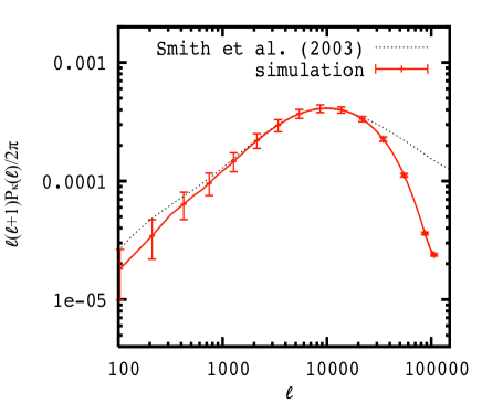
The interested reader is referred to Paper I for more details about the simulations and the process of making the maps. We made one important change, however, which must be high-lighted. While in Paper I, the density and potential planes had a resolution of $2048\times 2048$ (same as the resolution used for ray-tracing and the final convergence map), here we adopted a higher resolution, $4096\times 4096$, for both the density and the potential planes. This change has been proven to be important as lower resolution yields a loss in power at large wave number, as demonstrated by WFWLBSNG . In Fig. 1, we compare the 2D angular power spectrum of the WL convergence field at $4096^{2}$ resolution with the theoretical power spectrum. The latter was obtained by direct line–of–sight integration, using the Limber approximation, and the fitting formulae for the nonlinear 3D matter power spectrum from Smith+03 , calculated with the code NicaeaNicaea . In the range $400~{}\hbox to0.0pt{$<$\hss}{\lower 4.30554pt\hbox{$\sim$}}\ell~{}\hbox to0.0pt{$<$\hss}{\lower 4.30554pt\hbox{$\sim$}}30,000$, the power spectrum derived from our maps is not significantly suppressed by either the finite box-size or resolution, and it agrees well with the theoretical expectation.

Figure 1: Angular power spectrum of the WL convergence as a function of spherical harmonic index $\ell$. The solid curve is the average over 1000 simulated 12-square-degree convergence maps from ray-tracing through 45 independent N-body simulations for the fiducial cosmology. The error bars indicate the variance between the maps in the bins plotted. The dashed curve is the theoretical prediction, based on the 3D nonlinear matter power spectrum  Smith+03 , with the Limber approximation Limber1953 . Source galaxies are assumed to be located at $z_{s}=2$. No intrinsic ellipticity noise or smoothing were added.

Once the maps have been created, we take the redshift-dependent r.m.s. of the noise in one component of the shear to be DCPFCSD

$$\sigma_{\lambda}(z) = 0.15+0.035z.$$ (1)

Note that this corresponds, in the weak lensing limit, to an r.m.s. ellipticity of $0.30+0.07z$ (Jarvis+03, ).

For simplicity, in our analysis we assume that the source galaxies are located on a source plane at a fixed redshift, with $n_{\rm gal}=15~{}{\rm arcmin^{-2}}$. We apply a $\theta_{G}=1~{}{\rm arcmin}$ Gaussian smoothing to the maps. The noise $\sigma^{2}_{\rm noise}$ in the convergence after the Gaussian smoothing then becomes

$$\sigma^{2}_{\rm noise} = \frac{\langle\sigma^{2}_{\lambda}\rangle}{2\pi\theta^{2}_{G}n_{\rm gal}}.$$ (2)

For reference, we note that at redshift $z_{s}=2$, the above gives $\sigma_{\rm noise}=0.023$, very close to the r.m.s. of the convergence $\sigma_{\kappa}=0.022$ in the noise-free maps. The r.m.s. of the total convergence field, with noise included, is $\sigma_{\kappa}=0.031$.

II.2 Suite of Simulated Maps

In addition to the fiducial cosmology, we have run N-body simulations in six other models. Each of these differs from the fiducial model in a single parameter: we vary $\sigma_{8}$, $w$, $\Omega_{m}$ in both directions, with values $\sigma_{8}$ = 0.750 and 0.850; $w$ = -0.8 and -1.2; and $\Omega_{m}$ = 0.23 and 0.29. We assume the universe always stays spatially flat (i.e. $\Omega_{\Lambda}+\Omega_{m}=1$). The seven different cosmologies will hereafter be referred to as the fiducial, high-$\sigma_{8}$, low-$\sigma_{8}$, high-$w$, low-$w$, high-$\Omega_{m}$, and low-$\Omega_{m}$ models, respectively, as summarized in Table  1. In each of these N-body runs, we create 1000 different WL maps with source galaxies at $z_{s}=1$, and another 1000 maps with galaxies at $z_{s}=2$. Each map covers a solid angle of $3.46\times 3.46$ degrees. All maps were created by mixing potential planes randomly among five different N-body runs, with independent realizations of the initial conditions, in the given cosmology. Finally, we created an additional 1000 control maps, using the planes from 45 additional independent N-body runs in the fiducial model. Having 9 times more strictly independent realizations allows us to compute the covariance matrix more accurately (needed for computing $\Delta\chi^{2}$; see below), and to check the robustness of our results to different realizations of the fiducial model.

	$\sigma_{8}$	$w$	$\Omega_{m}$	# of sims
Fiducial	0.798	-1.0	0.26	5
Control	0.798	-1.0	0.26	45
High-$\sigma_{8}$	0.850	-1.0	0.26	5
Low-$\sigma_{8}$	0.750	-1.0	0.26	5
High-$w$	0.798	-0.8	0.26	5
Low-$w$	0.798	-1.2	0.26	5
High-$\Omega_{m}$	0.798	-1.0	0.29	5
Low-$\Omega_{m}$	0.798	-1.0	0.23	5

Table 1: Cosmological parameters varied in each model. The universe is always assumed to be spatially flat ($\Omega_{\Lambda}+\Omega_{m}=1$).

II.3 Halo Finding

We use the publicly available AMIGA halo finder (AHF ; hereafter AHF) to identify collapsed halos in our N-body runs. AMIGA finds halos based on an iterative density refinement scheme. Its output consists of the 3D positions of the halos, and, importantly for us, the tagged set of particles belonging to each halo. The virial radius of a halo is such that when a sphere is placed at the halo’s location, with a radius $r_{\rm vir}$, the overdensity $\bar{\rho}(r_{\rm vir})$ is

$$\bar{\rho}(r_{\rm vir}) = \Delta_{\rm vir}\rho_{b},$$ (3)

where $\rho_{b}$ is the background baryon density, and where $\Delta_{vir}=180$ is adopted in this study. The mass of the halo is then simply given by

$$M_{\rm vir} = 4\pi\rho_{b}\Delta_{\rm vir}r^{3}_{\rm vir}/3.$$ (4)

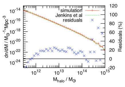
As a simple test of both our N-body simulations and our implementation of the halo finder, we reproduce the fitting formula (their equation B3.) for the halo mass function reported by Jenkins et al. Jenkins+01 . An example of this comparison is shown, in our fiducial model at $z=0$, in Fig. 2. Overall, we find excellent agreement, with an accuracy of 25% or better up to a halo masses of $2\times 10^{14}{\rm M_{\odot}}$. For larger masses, there is a large scatter.

Figure 2: Halo mass function, produced with the AMIGA halo finder AHF , in our N-body simulation of the fiducial model at $z=0$, compared to the fitting formula from Jenkins et al. Jenkins+01 .

One of the goals in this study is to identify halos contributing to each individual convergence peak. To do this, starting from each peak, we follow the light ray, and record the information (masses and location) of the halos found within a light cone centered on the peak, with a radius of 3 arcmin. This radius is chosen to be three times the smoothing scale. We have verified that doubling the radius of the light cone does not change our halo matching results below – in the sense that no additional halos are identified that contribute significantly to the total convergence of a peak (see detailed discussion below). To be consistent with the perpendicular projection of the particle density in each simulation snapshot, the light rays consist of a series of parallel line segments, which are perpendicular to the potential planes. The coordinates where the segments cross the potential planes are determined by the lensing deflection angle, computed and stored during the ray-tracing analysis. For the same reason, the light cones are composed of a series of parallel cylinders with a radius of 3 arcmin, centered on the corresponding light ray.

As explained above, we truncate the simulation snapshots, in order to generate more independent realizations of maps. As a result, occasionally, parts of halos that happen to be located near the plane of the truncation can be unphysically “cropped”. These cropped halos become important only when they are sufficiently massive to contribute to the convergence of a peak, and when they are located near (within a fraction of their virial radius) one of the two truncation planes (either in the front or the back). Given that halo virial radii are of order $\sim 1h^{-1}$Mpc, and our truncated box size is 80$h^{-1}$Mpc, the probability that the latter condition is satisfied is $\sim(1+1)/80\sim 2.5\%$. We therefore simply restrict our halo catalog only to halos that do not touch the edges. We have checked that neglecting the cropped halos does not significantly affect our results.

Our simulations resolve the density structure of individual halos with masses of $M~{}\hbox to0.0pt{$>$\hss}{\lower 4.30554pt\hbox{$\sim$}}{\rm few}\times 10^{11}~{}{\rm M_{\odot}}$. However, each map contains on the order of $10^{3}$ peaks, and more than a dozen halos can contribute to the total convergence of a single peak; therefore, computing the exact contribution of each halo to each peak is computationally impractical. Instead, we replace each halo by a spherically symmetric NFW UDPHC halo with the same virial mass $M_{\rm vir}$. For a given impact parameter $d$ (defined as the angular distance between the halo center and the point of closest approach of the light ray corresponding to the peak), redshift $z$, and mass $M_{\rm vir}$, the contribution of the off-center halo to the convergence peak can then be calculated analytically.

More specifically, the density profile is assumed to follow

$$\rho_{\rm nfw}(r) = \frac{\rho_{s}}{(r/r_{s})[1+(r/r_{s})]^{2}},$$ (5)

where $r$ is the radius from the halo center, and $r_{s}$ and $\rho_{s}$ are a characteristic radius and density. The profile is truncated at $r_{200}$, inside which the mean overdensity with respect to the critical density of the universe at redshift $z$ is 200. We adopt the concentration parameter $c_{\rm nfw}=r_{200}/r_{s}=5$ in this paper. The convergence due to the halo, given an extended redshift distribution of the background galaxies, is then given by

$$\kappa(\phi) = \frac{4\pi G}{c^{2}}\frac{\Sigma(\phi)\chi_{z}}{(1+z)}\frac{\int^{\infty}_{z}\,dz^{\prime}(dn/dz^{\prime})(1-\chi_{z}/\chi_{z^{\prime}})}{n_{\rm tot}}.$$ (6)

Here $\Sigma(\phi)$ is the projected surface density of the halo (given explicitly in ref. TJ03 ; see their equations 26-27), $\chi_{z}$ is the comoving distance to redshift $z$, $dn/dz$ is the surface number density of background galaxies per unit redshift, and $n_{\rm tot}$ is the mean total surface density. The latter is taken to be $n_{\rm tot}\delta(z-z_{s})$ in this paper, with $z_{s}$ as the source redshift. Finally, we use a Gaussian window function to smooth the convergence induced by the halo,

$$\kappa_{G} = \int\,d^{2}\phi W_{G}(\phi)\kappa(\mid\vec{\phi}-\vec{\phi_{0}}\mid)$$ (7)

$$W_{G}(\phi) = \frac{1}{\pi\theta^{2}_{G}}\exp(-\frac{\phi^{2}}{\theta^{2}_{G}})$$ (8)

$$\mid\vec{\phi_{0}}\mid = \frac{d(1+z)}{\chi_{z}}$$ (9)

where the center of the smoothing kernel ($\vec{\phi}=0$) is set to the angular position of the light ray corresponding to a peak, and $\vec{\phi_{0}}$ is the angle toward the halo center. The smoothing scale $\theta_{G}$ is chosen to be 1 arcmin, as in the simulated maps.

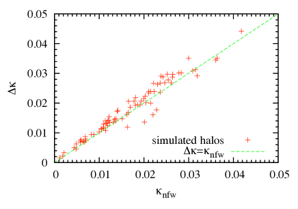
To check the accuracy of the NFW approximation for the convergence, we selected $81$ halos with masses in the range $1.5\times 10^{12}~{}{\rm M_{\odot}}<M<1.5\times 10^{14}~{}{\rm M_{\odot}}$ in one of the realizations of our fiducial model. For each halo, we record the value of the convergence $\kappa$ in the map (with sources galaxies at $z_{s}=1$), in the pixel located in the direction toward the halo center. We then remove the halo from the simulation box, and repeat the ray-tracing procedure discussed above, to compute a new value $\kappa_{0}$ at the same position, but without the halo. In Fig. 3, we show the actual difference $\Delta\kappa\equiv\kappa-\kappa_{0}$, against the value $\kappa_{\rm nfw}$ expected based on the NFW halo model. As the figure shows, the NFW assumption works accurately, although it results in a slight underestimate of the convergence. The points in the figure yield an average fractional bias of $\langle(\kappa_{\rm nfw}-\Delta\kappa)/\Delta\kappa\rangle=-0.067$ and an r.m.s. scatter of $\langle(\kappa_{\rm nfw}-\Delta\kappa)^{2}/\Delta\kappa^{2}\rangle^{1/2}=0.15$.

Figure 3: Comparison of the convergence $\kappa_{\rm nfw}$, produced by halos with an NFW profile, and the difference $-\Delta\kappa$ in the simulated convergence map induced by artificially removing the halo from the 3D simulation box. 81 halos, identified in a $z_{s}=1$ map generated in our fiducial model, were used for this exercise. No galaxy noise was added to the maps. The NFW assumption works well, with a fractional bias of only -6.7 percent, and a scatter of 15 percent, relative to $\Delta\kappa$.

II.4 Gaussian Random Field Predictions

One of the key questions to be answered in this paper, is the extent to which the peak counts contain information beyond traditional measures, such as the power spectrum. For example, if the peaks were produced only by a combination of pure galaxy shape noise (which is Gaussian by assumption) and linear fluctuations in the matter density, then their statistics would be fully described by a Gaussian random field (GRF). The majority of the high peaks are known to be associated with collapsed, nonlinear objects, and their statistics will clearly be non-Gaussian. However, the extent to which lower-amplitude peaks are non-Gaussian is not clear ab-initio. As mentioned in the Introduction, these peaks contain most of the cosmological information, and therefore the departure in the statistics of these peaks from Gaussian predictions is important to understand and quantify.

Figure 4: Number of convergence peaks in a Gaussian random field, as a function of their height measured in units of the standard deviation of the convergence, $\sigma_{0}$. The data points show the number of peaks in bins of width $\Delta\kappa=0.25\sigma_{0}$, obtained by averaging counts in 200 random Monte Carlo realizations of a 2d GRF. The input power spectrum was calculated from the non-linear matter power spectrum in Smith et al. Smith+03 in our fiducial cosmology, with source redshift $z_{s}=2$, including galaxy noise and smoothing. The map size, after excluding 40 pixels along each edge, is $2.88\times 2.88~{}{\rm deg}^{2}$.

As a simple test, we directly compare our simulated peak counts with those expected in a GRF. Fortunately, the peak counts in a two–dimensional GRF, and their distribution in height, are predictable analytically SCBRF . In fact, they depend only on the first and second derivatives of the correlation function on small scales (or, equivalently, the first two moments of the power spectrum). For completeness, we reproduce the relevant equations here. The differential number of maxima per unit solid angle, $n_{\rm max}(\nu)$, with height in the range $\nu$ to $\nu+d\nu$, where $\nu$ is measured in units of the standard deviation $\sigma_{0}$ of the random field, is given by

$$n_{\rm max}(\nu)d\nu = \frac{1}{2\pi\theta^{2}_{*}}\exp(-\nu^{2}/2)\frac{d\nu}{(2\pi)^{1/2}}G(\gamma,\gamma\nu)$$ (10)

where

$$G(\gamma,x_{*}) = (x^{2}_{*}-\gamma^{2})[1-\frac{1}{2}{\rm erfc}\{\frac{x_{*}}{[2(1-\gamma^{2})]^{1/2}}\}]$$ (11)

$$+x_{*}(1-\gamma^{2})\frac{\exp\{-x_{*}^{2}/[2(1-\gamma^{2})]\}}{[2\pi(1-\gamma^{2})]^{1/2}}$$

$$+\frac{-x^{2}_{*}/(3-2\gamma^{2})}{(3-2\gamma^{2})^{1/2}}$$

$$[1-\frac{1}{2}{\rm erfc}\{\frac{x_{*}}{[2(1-\gamma^{2})(3-2\gamma^{2})]^{1/2}}\}]$$

$$\gamma = \sigma^{2}_{1}/(\sigma_{0}\sigma_{2})$$ (12)

$$\theta_{*} = \sqrt{2}\sigma_{1}/\sigma_{2}$$ (13)

$$\sigma^{2}_{p} = \int^{\infty}_{0}\frac{\ell d\ell}{2\pi}\ell^{2p}P_{\ell}$$ (14)

$$= p!2^{2p}(-1)^{p}\frac{d^{p}\xi}{d(\theta^{2})^{p}}(0),$$

and where $P_{\ell}$ is the continuous 2d power spectrum of the convergence field, and $\xi(\theta)$ is its two-point correlation function. Integrating Eq. (10) over $\nu$ gives the total number of peaks $n_{\rm pk}$ regardless of their height,

$$n_{\rm pk} = (4\pi\sqrt{3})^{-1}{\theta_{*}}^{-2}.$$ (15)

To verify the accuracy of these analytic formulae, we produced 200 numerical maps of GRFs, by generating 200 independent random realizations of the theoretical 2d weak lensing power spectrum (in our fiducial model, assuming a source redshift $z_{s}=2$). We first generate a 2d complex random field in $\ell$ space, with the real and imaginary parts of Fourier modes distributed independently, following Gaussians with a standard deviation of $\sqrt{P_{\ell}/2}$. Here $P_{\ell}$ is the power spectrum BBKS . We then perform a discrete Fourier transform to produce maps in real space. The GRF maps have a size of $2048\times 2048$, to mimic the actual WL maps. Noise is then added according to Eqs. (1) and (2), with $n_{\rm gal}$=15, and a 1 arcmin smoothing is applied. To avoid edge effects, we discard pixels located within 40 pixels ($\approx 3\times$ the smoothing scale) of the map edges.

To reproduce the random GRF realizations as closely as possible, we do not calculate $\sigma_{0}$, $\sigma_{1}$, $\sigma_{2}$ from the input power spectrum; instead, we measure these directly from the maps, using the finite difference derivatives (ignoring the constant coefficients in Eq. (14))

$$\sigma^{2}_{0} = \langle\kappa^{2}\rangle-{\langle\kappa\rangle}^{2}$$ (16)

$$\sigma^{2}_{1} = \langle\left(\frac{d\kappa}{dx}-\overline{\frac{d\kappa}{dx}}\right)^{2}+\left(\frac{d\kappa}{dy}-\overline{\frac{d\kappa}{dy}}\right)^{2}\rangle$$ (17)

$$\sigma^{2}_{2} = \langle\left(\frac{d^{2}\kappa}{dx^{2}}-\overline{\frac{d^{2}\kappa}{dx^{2}}}+\frac{d^{2}\kappa}{dy^{2}}-\overline{\frac{d^{2}\kappa}{dy^{2}}}\right)^{2}\rangle$$ (18)

where $\kappa$ is the 2d convergence field, and $\overline{\frac{d\kappa}{dx}},\overline{\frac{d\kappa}{dy}},\overline{\frac{d^{2}\kappa}{dx^{2}}}$, and $\overline{\frac{d^{2}\kappa}{dy^{2}}}$ are the averages of the corresponding first and second derivatives. For reference, this leads to a prediction of 1680 peaks, compared to the actual number 1685 found in the noiseless maps; the prediction based on the analytic calculation of the $\sigma$’s is slightly worse, 1649. We have checked that the situation is similar in the true WL maps: measuring $\sigma_{0,1,2}$ numerically gives a slightly more accurate prediction for the total number of peaks than calculating $\sigma_{0,1,2}$ analytically from the power spectrum through Eq. (14).

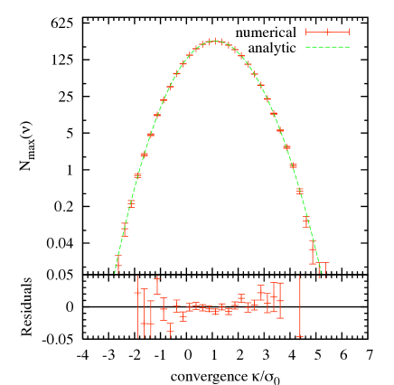
In Fig. 4, we show predictions from the analytic formulae (Eqs. (10)-(14)), and the mean peak counts in our 200 mock GRF maps. This tests our reproduction of the formulae, as well as the accuracy of our numerical measurements of $\sigma_{0}$, $\sigma_{1}$, $\sigma_{2}$. The agreement is excellent, with residuals of only $~{}\hbox to0.0pt{$<$\hss}{\lower 4.30554pt\hbox{$\sim$}}~{}2$ percent over most of the range shown.

The main advantage of creating mock numerical realizations of the GRF maps is that we can use these to measure the (co)variance in the Gaussian peak counts. This covariance matrix is necessary to compute the $\Delta\chi^{2}$ values between pairs of cosmologies in the Gaussian case (see discussion below).

II.5 Statistical Comparisons

The basic statistical task in this paper is to assign a significance of the difference between a pair of maps, given the stochastic fluctuations in the maps over many realizations. This is required in order to quantify how well two cosmological models can be distinguished with the peak counts.

The simplest statistical test consists of computing $\Delta\chi^{2}_{f^{\prime},f}$ between a pair of cosmologies $f$ and $f^{\prime}$, using the mean number of peaks in each bin, averaged over all realizations,

$$\Delta\chi^{2}_{f^{\prime},f} = \mathbf{dN}^{(f^{\prime},f)}(C^{(f)})^{-1}\mathbf{dN}^{(f^{\prime},f)}$$ (19)

$$= \sum_{ij}dN_{i}^{(f^{\prime},f)}(C^{(f)})_{ij}^{-1}dN_{j}^{(f^{\prime},f)},$$

where $dN_{i}^{(f^{\prime},f)}\equiv\overline{N}_{i}^{(f^{\prime})}-\overline{N}_{i}^{(f)}$ is the difference between the average number of peaks in bin $i$ in cosmology $f^{\prime}$ and in cosmology $f$. Note that $i$ here can label bins of different peak–heights, but can also include different source galaxy redshifts or smoothing scales. Here $C^{(f)}$ denotes the covariance matrix of the number of peaks in cosmology $f$,

$$C^{(f)}_{ij}=\frac{1}{R-1}\sum_{r=1}^{R}(N^{(f;r)}_{i}-\overline{N}^{(f)}_{i})(N^{(f;r)}_{j}-\overline{N}^{(f)}_{j})$$ (20)

where $N^{(f;r)}_{i}$ is the number of peaks in bin $i$ in the $r^{\rm th}$ realization (i.e. convergence map) of the cosmology $f$, and $R$ is the total number of realizations.

This $\Delta\chi^{2}_{f^{\prime},f}$ could be interpreted directly as a likelihood or confidence level only if (i) the peak count distribution in each bin were Gaussian, and (ii) the mean peak counts depended linearly on the cosmological parameters. As long as the change in parameters is small, a Taylor expansion to the first order is a good approximation, and therefore the second condition is unlikely to be strongly violated in our case. We will verify below that condition (i) is satisfied to a good accuracy, as well. To be specific, we examine directly the distribution of the quantity defined as

$$\chi^{2}_{f^{\prime}}(r) = \sum_{ij}dN_{i}^{(f^{\prime};r)}(C^{(f)})_{ij}^{-1}dN_{j}^{(f^{\prime};r)}$$ (21)

where $dN_{i}^{(f^{\prime};r)}\equiv N_{i}^{(f^{\prime};r)}-\overline{N}_{i}^{(f)}$ is the difference between the number of peaks in bin $i$ in realization $r$ of a test cosmology $f^{\prime}$, and the average number of peaks in the same bin in the fiducial cosmology $f$. We will show that $\chi^{2}_{f}(r)$ closely follows a true chi-squared distribution.

Unless stated otherwise, in this paper, we use five $\kappa$ bins to calculate $\Delta\chi^{2}$. The bin boundaries are chosen by visual inspection, using two rough criteria: (i) the difference in the peak height distributions in the two cosmologies should not change sign within any of the bins, and (ii) the numbers of peaks in each bin should be as comparable as possible. The influence of the number of bins and the bin boundaries on our results will be discussed in § IV below.

II.6 Fisher Matrix and Marginalized Error

With the assumptions that (i) the observables, i.e. the mean number of peaks in each bin $\overline{N}_{i}$, depend linearly on the cosmological parameters $p$; and (ii) that for a fixed $p$, the probability distribution of $N_{i}$ follows a Gaussian, the marginalized error on each parameter can be calculated using the Fisher matrix (e.g. ref. Tegmark+97 ).

The Fisher matrix for point $p_{0}$ in the parameter space is given by the matrix trace

$$F_{\alpha\beta} = \frac{1}{2}Tr[C^{-1}C_{,\alpha}C^{-1}C_{,\beta}+C^{-1}M_{\alpha\beta}],$$ (22)

with

$$M_{\alpha\beta} \equiv \overline{N}_{,\alpha}\overline{N}^{T}_{,\beta}+\overline{N}_{,\beta}\overline{N}^{T}_{,\alpha},$$ (23)

where the Greek indices refer to model parameters, a comma preceding an index denotes a partial derivative with respect to the corresponding parameter, $C_{ij}$ is the covariance matrix of $N_{i}$’s, and $\overline{N}_{i}$ is the expectation value of $N_{i}$. In this paper, we will consider only the second term in Eq. (22) above. The constraints through this term arise from the dependence of the mean number of peaks $\overline{N}_{i}$ on the cosmological parameters. In principle, additional constraints could be available from the first term, which represents the dependence of the (co)variances $C_{ij}=\langle N_{i}N_{j}\rangle$ on cosmology (see refs. LH04 and HK03 for related points in the context of cluster counts). Our results suggest that this dependence is relatively weak; in practice, however, we do not have a sufficient number of independent realizations to accurately evaluate this dependence. From the Fisher matrix, the marginalized error on the parameter $\alpha$ is calculated simply as $\sigma_{\alpha}=(F^{-1})_{\alpha\alpha}^{1/2}$. (In contrast, the square root of Eq. (19) divided by the difference between model parameters corresponds to the parameter sensitivity with all other parameters fixed.)

III Results

III.1 The Physical Origin of Peaks and of their Cosmology Dependence

In general, peaks in the convergence field can arise for different reasons. They could be caused by (i) one or more collapsed halos along the LOS; (ii) large-scale, mildly overdense filaments, seen in projection; (iii) non–linear “protoclusters” that are on their way to collapse, but have not yet virialized and settled into an equilibrium structure WK02 ; DFN09 ; and (iv) pure galaxy shape noise. In reality, peaks can be produced by a combination of the above effects.

Relatively high–amplitude ($~{}\hbox to0.0pt{$>$\hss}{\lower 4.30554pt\hbox{$\sim$}}3.5\sigma$) lensing peaks have been studied thoroughly in the past (e.g. White+02 ; SMCWLS ; HS05 ), and it is known that a large fraction of these peaks is attributable to a single collapsed massive halo. Our motivation to revisit this topic is that the cosmological information is contained primarily in the lower–amplitude peaks, whose origin has not yet been clarified. As described in section II, we start with each individual peak, and identify all halos along the sightline. Likewise, for each halo, we identify peaks that are located within a 3 arcmin distance from the 2d sky position of the halo.

We would also like to know why the number of peaks changes with cosmology. To help clarify this, we examine realizations of pairs of models with different values of $\sigma_{8}$ with quasi identical initial conditions. In these pairs of models, we use the same random seeds to generate the amplitudes and phases for the Fourier modes of the density and velocity field at redshift $z=0$, and then scale these back to the starting redshift of the simulation, with the linear growth factor. Since the power spectra differ only by an overall normalization, and since the growth factor is independent of $\sigma_{8}$, the initial conditions, as well as the final WL maps, maintain very similar patterns. Therefore we can attempt to match individual peaks in the two cosmologies, to see what happens to a given peak, when, say, $\sigma_{8}$ is increased.

Results in this section are based on 50 realizations of the noisy maps in the fiducial and in the low-$\sigma_{8}$ models, with source galaxy redshift $z_{s}=2$, $n_{\rm gal}=15$ and 1 arcmin smoothing. The maps have an angular size $3.46\times 3.46~{}{\rm deg}^{2}$, $2048\times 2048$ pixels. To avoid edge effects, 30 pixels($\approx$ 3 times the smoothing scale) from all four edges of each map are discarded, leaving an area of $3.36\times 3.36~{}{\rm deg}^{2}$. The fiducial model is used for studying the origins of the peaks, and a comparison between the fiducial and the low–$\sigma_{8}$ model is used for studying the cosmology-sensitivity.

We first perform an analysis of peak-halo matching, closely following Hamana et al. SMCWLS , for both high and medium peaks. High peaks are defined as those with $\nu\geq 4.8$, where $\nu$ is the maximum value $\kappa_{\rm peak}$ of the peak, in units of the standard deviation of the noise field. We restrict our halo catalog to halos that are expected (based on the NFW approximation; Eqs. (5)-(6) with $\phi_{0}=0$) to produce a peak with a height of $\nu_{\rm nfw}\geq 4.8$. Similarly, for medium peaks with $1.1\leq\nu<1.6$, we restrict our halo catalog to those halos with $1.1\leq\nu_{\rm nfw}<1.6$. We carry out the peak-halo matching by searching for a matched pair candidate within a radius of 1.8 arcmin from the peak position or from the halo center. This maximum angular separation is chosen, as in SMCWLS , so that it is larger than the smoothing radius of 1 arcmin, while it is still smaller than the angular virial radius of a massive halo at $z~{}\hbox to0.0pt{$<$\hss}{\lower 4.30554pt\hbox{$\sim$}}1.3$, where the lensing kernel has the most weight. If there is more than one candidate pair within this radius, we follow SMCWLS and adopt the closest one as the primary candidate.

class	matching result	number of matches
		(high peaks)	(medium peaks)
$i$	halo $\Leftrightarrow$ peak	526 (0.93)	2653 (4.7)
$ii$	halo with no paired peak	230 (0.41)	19609 (35)
$iii$	peak with no paired halo	2264 (4.0)	24709 (44)
$iv$	halo $\Rightarrow$ peak	2 (0.0035)	90 (0.16)
$v$	halo $\Leftarrow$ peak	12 (0.021)	194 (0.34)

Table 2: Matching of halos and peaks similar to Hamana et al. SMCWLS , but shown separately for high and medium peaks. In the second column, “$\Leftrightarrow$” indicates a primary match in both directions, whereas $\Rightarrow$ and $\Leftarrow$ indicate a primary match in the direction of the arrow only. In total, our 50 realizations of $3.36\times 3.36deg^{2}$ maps contain 2,802 high peaks and 27,556 medium peaks, whereas the three–dimensional N-body outputs contain 758 massive halos and 22,352 medium halos with corresponding masses. The numbers in () show the number per $deg^{2}$ averaged over 50 realizations, to be compared with the results of Hamana et al. SMCWLS (see text for discussion).

The 50 noisy maps contain a total of 2,802 high peaks and 27,556 medium peaks. For comparison, the halo catalogs contain 758 massive halos with $\nu_{\rm nfw}\geq 4.8$ and 22,352 medium-sized halos with $1.1\leq\nu_{\rm nfw}<1.6$. Following Hamana et al. SMCWLS , we sort the results of the matches into the following five categories: ($i$) both a halo and a peak are each other’s primary pair candidate; ($ii$) a halo without a paired peak ($iii$) a peak without a paired halo; ($iv$) a halo has a matched peak, but is not the primary matched halo of that peak; and ($v$) a peak has a matched halo, but it is not the primary matched peak of that halo. Table 2 shows the number of matches, separately for high and medium peaks, falling into each category.

Bearing in mind differences in redshift, noise, and peak height thresholds, our results are in reasonable agreement with SMCWLS . Overall, we have found, on average, 5.0 deg^-2 high peaks and 1.3 deg^-2 massive halos. The majority ($70\%$) of the massive halos produce a one-to-one matching peak, although these account only for $\approx 20\%$ of the total population of high peaks. More specifically, SMCWLS finds 23 deg^-2 high peaks and 8.1 deg^-2 massive halos. Their matches per $deg^{2}$ in categories $i$, $ii$, and $iii$ are 5.9, 2.1, 15 accordingly. In general, we have found fewer peaks and halos than SMCWLS , which can be attributed to our lower $\sigma_{8}$ and $\Omega_{m}$ values. Our threshold of high peaks is also not identical to theirs. However, we have checked that the number of halos above a threshold is in good agreement with their equation 15 SMCWLS , when our cosmological parameters are used. We have found a slightly lower completeness of the halos (less fraction of halos in category $i$ and more fraction in category $ii$), and also a $\sim 50\%$ lower purity (more fraction of peaks in category $iii$). We have chosen a higher source redshift, $z_{s}=2$ (SMCWLS used $z_{s}=1$), this makes projection effects more important, and may explain why our completeness is lower. Our noise is slightly larger, and our simulations and final maps have higher resolution, compared to SMCWLS – these effects tend to increase the number of peaks relative to number of halos, and to reduce the purity of identifying halos.

The most important result in Table 2 is that, in difference from massive halos, only a small fraction ($12\%$) of the 22,352 medium-sized halos produce a medium peak with a one-to-one pair, accounting for less than $10\%$ of all medium peaks. We conclude that the close agreement in the number of medium peaks and halos (27,556 vs. 22,352) is a coincidence - and noise and projection effects are much more important for medium peaks than for high peaks.

We next extend the above analysis, by identifying all halos, down to low masses, by using a larger, 3 arcmin cone around the LOS toward each peak, and by computing the expected contribution of each halo $\kappa_{i}$ to the total convergence at the position of the peak (based on the NFW approximation). We then rank the halos according to their $\kappa_{i}$ values (starting from highest and going down to the lowest). We add the noise $\kappa_{\rm noise}$ at the peak location to this ranked list, and ask the following question: starting from the highest value, how far down this ranked list do we need to sum the contributions, before they account for $>50\%$ of the total peak height?

Figure 5: These figures illustrate the number of halos, as well as noise, contributing to medium and high peaks in 50 realizations. For each peak, we identify all halos along the sightline, and rank them (as well as noise) according to their contribution to the peak convergence. In the upper two panels, we show the distribution in the number of halos required to account for $>50\%$ of the total peak height (with “0” corresponding to cases in which noise alone explains half of the peak value). In the lower two panels, noise is excluded, and we show the distribution in the number of halos required to account for $>50\%$ of the total halo contribution. Error bars are estimated as the the standard deviation of the number of counts in each bin, multiplied by $\sqrt{50}$.

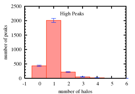
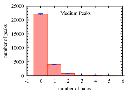
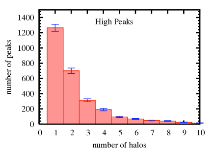
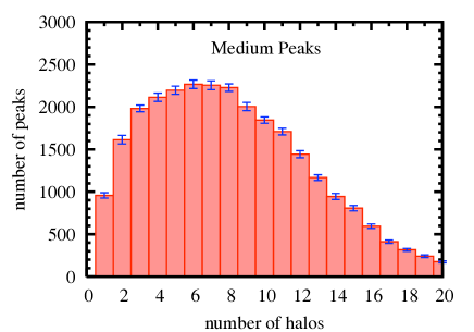
In the upper two panels of Fig. 5, we plot the distribution of this quantity; a “0” indicates that noise is the single largest contributor, and already accounts by itself for most of the peak, “1” indicates that at least 1 halo had to be included, etc. These panels clearly show that the large majority of high peaks are dominated by a single halo, which accounts for at least half of the peak amplitude. Most of these halos fall below the expected threshold $\nu_{\rm nfw}=4.8$. The high peaks thus have a much better one-to-one match with halos than Table 2 implies, once lower–mass halos are included. On the other hand, the large majority of medium peaks are dominated by noise.

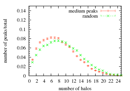
Since noise does not contain any cosmological information, in the bottom two panels of Fig. 5, we repeat the same exercise, except that the noise contribution is excluded, and we show the number of halos required to account for the total halo contribution. These panels show that while the high peaks are typically dominated by a single halo, the contributions from a second (or higher-rank) halos is often ($~{}\hbox to0.0pt{$>$\hss}{\lower 4.30554pt\hbox{$\sim$}}50\%$ of cases) as important. In the case of medium peaks, however, it is very rare ($<5\%$ of cases) for a single halo to dominate the cumulative halo contribution. Instead, there is a broad distribution, but typically (in $\sim$half the cases) $4-8$ halos are required to account for $>$half of this total halo contribution. As a sanity check, we have computed the analogous distribution for random directions on our maps (i.e., not toward peaks). For these random directions, as shown in Figure 6, the distribution has an even broader shape, centered at 8, and generally shifted toward larger numbers of halos. This reassures us that the medium peaks still do preferentially pick out directions toward conjunctions of $\sim 4-8$ halos. We also examined the masses and redshifts of these dominant $\sim 4-8$ halos. We have found that the masses range between ${\rm few}\times 10^{12}~{}{\rm M_{\odot}}<M<{\rm few}\times 10^{13}~{}{\rm M_{\odot}}$, and found no correlations in redshift (i.e., the contributing halos are not part of a single structure). Finally, we find that simply adding up the expected $\kappa$ contribution of all halos along the LOS to a peak always overproduces the $\kappa$ value of the peak (not surprising, since this neglects the $\kappa$ deficit from underdense regions).

Figure 6: As in the lower panels in Figure 5, we show the distribution in the number of halos required to account for $>50\%$ of the total halo contribution. Here we contrast these distributions for medium-height peaks and for randomly chosen directions on the sky. The figure demonstrates that medium–height peaks preferentially pick out directions toward conjunctions of $\sim 4-8$ halos.

We next wish to clarify why there are fewer medium-height peaks when $\sigma_{8}$ is increased (and vice versa). One can intuitively guess that increasing $\sigma_{8}$ simply increases the ”scatter” due to large scale structures. In the linear regime, changing $\sigma_{8}$ simply changes the local (3d) density contrast, by the same factor everywhere. Pretending that this holds in the nonlinear regime, it is easy to see that the set of peaks would be invariant under changing $\sigma_{8}$ – however, positive peaks would be enhanced, and negative peaks (i.e., maxima residing inside large-scale voids) would become yet more negative. This would broaden the peak-height distribution, and reduce the number of peaks near $\kappa_{\rm peak}\sim 0$. Of course, this picture is over-simplified: as $\sigma_{8}$ is increased, the change in the density field is not a simple re-scaling; furthermore, peaks can be destroyed and new peaks can be created. Indeed, we already know that the total number of peaks changes with $\sigma_{8}$ (Paper I).

To understand the dominant effect, we attempt to follow and match individual peaks in a pair of models with different $\sigma_{8}$. We have found that a direct matching of peaks is not possible, because the locations of the peaks tend to shift (by several to more than 20 pixels) and therefore the correspondence between peaks in two different maps remains ambiguous (except for the very highest and most conspicuous peaks). Instead, we proceed by using halos as intermediate proxies for the peaks. Starting from a peak in the first cosmology, we identify the halo that contributes most to this peak. For this analysis, we consider only those peaks for which the matched primary halo contributes at least 10% of the total halo contribution (otherwise it is unfair to use the halo as a proxy for the peak). We next search the entire halo catalog in the second cosmology, and identify the “same” halo, by finding the one that shares most common particles with the halo in the first cosmology. Finally, we search through the peaks in the second cosmology within a cone of 3 arcmin around the halo, requiring that their height is within the range $\pm\sigma_{\rm noise}$ of the original peak in the first cosmology, and that the “same” halo contributes at least 10% of the total halo contribution. If no such peak is found, then the match is declared unsuccessful. If more than one such peak is found, we select the one to which the matched halo contributes the most.

Figure 7: The figure shows the results of an attempt to match individual high and medium peaks in a pair of cosmologies, as explained in the text. The x-axis shows the peak height in the starting cosmology model, and the y-axis shows the height of the “same” peak in the model to be matched with the starting model (whenever the peak has a match). The top-left panel shows matches found in the fiducial model for the high peaks in the low-$\sigma_{8}$ cosmology (and vice versa in the top-right panel); the bottom two panels repeat the exercise for medium peaks. Typically $\sim 80\%$ of the high peaks have a match, but only $\sim 50\%$ of the medium peaks do.

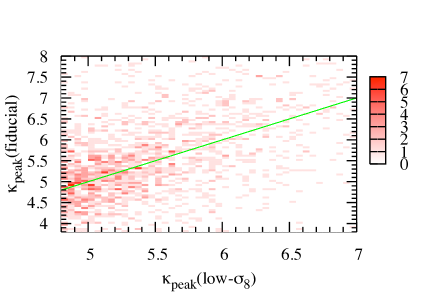
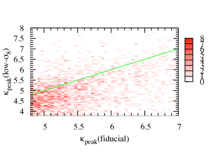
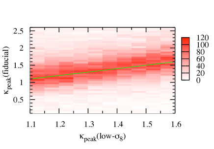
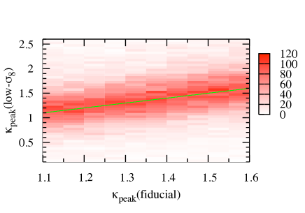
Fig. 7 shows the results of the above matching procedure between the fiducial and the low-$\sigma_{8}$ models, for both high peaks (upper two panels) and medium peaks (lower two panels). Focusing on the high peaks first, there are 1,987 high peaks in the lower $\sigma_{8}$ model, and 2,802 high peaks in the fiducial model. In the upper-left panel, we start with the peaks in the low-$\sigma_{8}$ model, and show their matches in the fiducial model. In the upper-right panel, we reverse the direction, and start with the fiducial model. We find an “unambiguous” match (in the sense defined in the preceding paragraph) for 87.1% and 80.8% of the peaks, respectively. Proceeding to the two lower panels, we show the results for the medium peaks. There are 29,097 medium-height peaks in the low-$\sigma_{8}$ model; only 56.2% of these have a matching peak in the fiducial model. Likewise, starting from the 27,556 medium-height peaks in the fiducial model (bottom panel), we find that 55.7% of these have a match in the low-$\sigma_{8}$ cosmology.

In conclusion, most high peaks are matched to a peak in the other cosmology, although the peak $\kappa$ values in the two cosmologies differ by an amount comparable to $\sigma_{\rm noise}$. In contrast, about half of the medium-height peaks do not have a clear match in the other cosmology. This is despite the fact that we use the same realization of the noise map in both cosmologies (i.e., we avoid creating an entirely different set of peaks by a different noise-realization), and despite our rather lenient definition of a “match”. We speculatively interpret this result as follows. Since the medium peaks are typically created by the sum of pure noise and many halos in projection, their existence and their amplitude are both sensitive to small changes in the spatial distribution and masses of these halos. In indirect support of the above conclusion, we have identified the following trend: on average, the proxy-halo contributes 49.6% for high peaks that have a match, vs. 33.8% for those that do not. Similarly, for medium peaks, the proxy halo contributes 25.1% vs. 18.9% for match vs. unmatched peaks. This shows that whenever the dominant halo accounts for a smaller fraction of the peak $\kappa$, it is more ”fragile” and is less likely to have a match in the other cosmology. Finally, we have found that when $\sigma_{8}$ is increased, then the matched halo in the higher-$\sigma_{8}$ cosmology has typically grown more massive, with an increase by 15% and 12% on average for matched and unmatched high peaks, 16% and 14% for matched and unmatched medium peaks. This trend, however, does not hold in the $\kappa$ values of the matched peaks; as Fig. 7 shows, the peak heights have a significant scatter, but a relatively low bias, between the cosmologies. This could be explained by the fact that underdense voids become even more underdense when $\sigma_{8}$ is increased, which tends to “cancel” the increase in $\kappa_{\rm peak}$ caused by the fattening of halos. To be specific, we find a fractional bias $\langle(\kappa_{2}-\kappa_{1})/\kappa_{1}\rangle=0.034$ and an r.m.s. scatter $\langle(\kappa_{2}-\kappa_{1})^{2}/\kappa_{1}^{2}\rangle^{1/2}=0.19$. when high peaks in lower $\sigma_{8}$ model are matched to high peaks in fiducial model. In the reverse direction, the bias and scatter are -0.088 and 0.17. These results agree with the upper two panels in Fig. 7, showing a positive bias when $\sigma_{8}$ is increasing, and a negative bias when $\sigma_{8}$ is decreasing. The bias for the medium peaks is less clear than for the high peaks. In fact, the bias is positive in both matching directions, with the number for increasing $\sigma_{8}$ (0.068) more positive than the number for decreasing $\sigma_{8}$ (0.032). This is because the medium peaks are dominated by noise, rather than halos, and the peaks which increase in height because of the positive noise have a larger chance to survive as a peak than those that are hurt by the noise. The scatter for medium peaks is $\approx 0.32$, about twice the scatter for high peaks.

class	low-$\sigma_{8}\rightarrow$ fiducial	fiducial $\rightarrow$ low-$\sigma_{8}$
exit to low $\kappa$	3303	3420
stay in bin	7683	7515
exit to high $\kappa$	5373	4408
total matched	16359	15343
lost (unmatched)	12738	12213

Table 3: We sort medium peaks into different categories, based on the outcome of our attempt to find a match for each peak in another cosmology. The total number of medium peaks in the low-$\sigma_{8}$ model and the fiducial model are 29,097 and 27,556 respectively. While going from one cosmology to the other, peaks can be “lost”, they can stay within the same $\kappa$ bin, or they can move out of the bin to higher or lower $\kappa$ values. Additionally, new medium peaks appear.

Finally, we examine the “movement” of the peaks in height $\kappa$ as $\sigma_{8}$ is varied, in order to test our hypothesis, stated above, that an increase in $\sigma_{8}$ tends to evacuate peaks from near the $\kappa\sim 0$ (or near the maximum of the peak-height distribution). For example, we divide the 29,097 medium-height peaks in the low-$\sigma_{8}$ model into several cases. Approximately half (12,738) of these peaks are unmatched: they “disappear” when $\sigma_{8}$ is increased (equivalently, these are peaks that “appear” when one starts from the fiducial model, and decreases $\sigma_{8}$). The remaining 16,359 matched peaks are further divided into middle, lower and high cases, based on whether they remain in the original medium-$\kappa$ bin (7,683), exit this bin toward higher $\kappa$ (5,373) or to lower $\kappa$ (3,303), in the other cosmology. These results, as well as the corresponding results in the reverse matching direction, are summarized in Table 3.

By examining the table, we conclude there is indeed a preferentially larger scatter in the direction out of the “medium” bin, when going from the lower $\sigma_{8}$ to the fiducial model, compared to the reverse direction: $(3,303+5,373)>(3,420+4,408)$. This table further reveals that there are two distinct reasons for the decrease in medium-height peaks. Approximately 2/3rd of the total decrease (of 29,097-27,556 = 1,541 $\approx$ 1500 peaks), or $\approx$ 900 peaks, can be attributed to the above mentioned ”scatter” due to the increased density contrast – i.e. more peaks moving out of the bin than into the bin. The remaining $\sim$1/3rd of the decrease is due to losing peaks, i.e. $\approx$ 500 more peaks are destroyed than created, as $\sigma_{8}$ is increased. Based on the preceding discussion, we speculate that this latter affect is caused by the projections of multiple halos, which can create and destroy the relatively low amplitude peaks.

In summary, the results in this section suggest that medium-height peaks are almost always dominated by pure galaxy shape noise, but they receive a significant contribution from collapsed halos, with typically 4-8 halos in projection along the LOS. The halos drive the cosmological sensitivity of these peaks in two ways: by (i) changing the amplitudes of the noise peaks, and by (ii) destroying and creating new peaks. Between these last two effects, in the case of $\sigma_{8}$, we found that the first is $\sim$twice as important as the second.

III.2 Comparison to Gaussian Predictions

Our next task is to examine whether (i) the statistics of the peaks, and (ii) their cosmology-sensitivity differs significantly from predictions in a Gaussian random field. The degree of any departure from a GRF is especially important to quantify for the medium peaks, since the results of the last section suggest that these are heavily dominated by pure Gaussian noise.

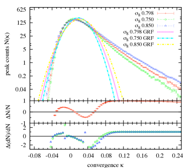
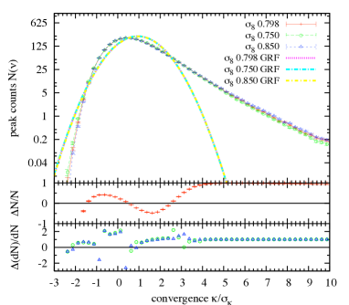
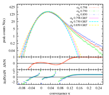
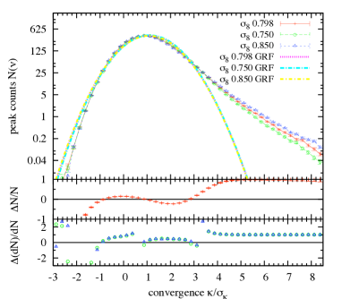
Our main results are shown in Fig. 8, which directly compare the peak counts in our simulated maps with those in a GRF. The GRF predictions are computed from the theoretical formula as discussed above, but using the (moments of) the power spectrum $\sigma_{0}$, $\sigma_{1}$, $\sigma_{2}$ that were measured from the corresponding simulated maps. In each panel, we also compare the high-$\sigma_{8}$, fiducial, and low-$\sigma_{8}$ models. In the bottom of each panel, we also show (i) the fractional difference between the GRF and the fiducial model and (ii) how the change in the peak counts between pairs of cosmologies is different in the GRF and our simulated maps. The source galaxies are assumed to be at $z_{s}=2$, and all results shown in the figure include 1 arcmin smoothing. We plot the mean number of peaks in convergence bins of width $\Delta\kappa=\frac{1}{4}\sigma_{\rm noise}=0.0045$, averaged over 1000 realizations. In the top two panels, we exclude noise from the maps; in the bottom two panels, noise is included. Finally, in the right two panels, we have scaled the convergence field $\kappa$ by its r.m.s. value $\sigma_{\kappa}$ (these histograms use a bin width of $\Delta(\kappa/\sigma_{\kappa})=0.25$). This removes information that arises from $\sigma_{\kappa}$ alone. If the sole effect of changing $\sigma_{8}$ was to change the heights of individual peaks by a constant factor, then this would result in a re-scaling of the peak-height probability distribution; the re-scaling by $\sigma_{\kappa}$ clarifies the relative importance of this effect.

As these figures show, in the noiseless case, the peak height distributions are very different from the Gaussian predictions and are reminiscent of the skewed one-point function of $\kappa$, which has a sharp drop at low demagnification, and a long tail to high magnification (e.g. ref. Wiley+09 and references therein). This correspondence of the high-tails is not entirely surprising; indeed, a pixel with a very high $\kappa$ value is likely to mark a peak. When noise is added, the distributions near their peaks look much more similar to the Gaussian predictions. However, there is still a large non-Gaussian deficit of the lowest peaks (with the most negative $\kappa_{\rm peak}$) and a clear excess of the highest ($\kappa~{}\hbox to0.0pt{$>$\hss}{\lower 4.30554pt\hbox{$\sim$}}3\sigma_{\kappa}$) peaks. Importantly, however, there also remains a clear difference in the peak-height distributions even for the medium-height ($\kappa\sim\sigma_{\kappa}$) peaks. Finally, as illustrated in the bottom insert in each panel, the cosmology-sensitivity of our peak histograms is also different from that in a GRF. These last points are encouraging, and suggest that the medium peaks do contain non-Gaussian information.

Figure 8: Number of peaks in our simulated $3.46\times 3.46{\rm deg^{2}}$(including the 3 arcmin edge) convergence maps, in bins of width $\Delta\kappa$ = 0.0045. In the right two panels, we have scaled the convergence field $\kappa$ by its r.m.s. value $\sigma_{\kappa}$; this removes information arising solely from $\sigma_{\kappa}$. The source galaxies are assumed to be at $z_{s}=2$, and all results include 1 arcmin smoothing. In each panel, the three curves with data points correspond (from top to bottom on the right) to the high-$\sigma_{8}$, fiducial, and low-$\sigma_{8}$ models. The other three curves show theoretical predictions for peak counts in Gaussian random fields with the same three power spectra. In the bottom of each panel, we show the fractional difference between our fiducial model and a GRF for the peak counts $\langle(N_{simu}-N_{GRF})/N_{simu}\rangle$ (demonstrating that the WL peaks are strongly non-Gaussian), as well as for the difference in the peak counts between pairs of cosmologies $\langle(\Delta N_{simu}-\Delta N_{GRF})/\Delta N_{simu}\rangle$ (explicitly demonstrating that the cosmology-sensitivity of our peak histograms is also different from that in a GRF). The four panels (upper-left, upper-right, lower-left, lower-right) show the results in noise–free unscaled, noise–free scaled, noisy unscaled and noisy scaled maps.

IV Discussion

IV.1 Sensitivity to Cosmological Parameters

map	cosmology	boundary
type	pair	locations
noisy us	F and High-$\sigma_{8}$	-0.0028	0.0217	0.0407	0.0695
noisy sc	F and High-$\sigma_{8}$	0.2650	0.6682	1.3550	3.3013
noisy us	F and High-$\Omega_{m}$	-0.0050	0.0200	0.0383	0.0627
noisy sc	F and High-$\Omega_{m}$	0.4618	0.9950	1.5750	3.0556
noisy us	F and High-$w$	-0.0019	0.0190	0.0347	0.0551
noisy sc	F and High-$w$	0.2565	1.1450	2.4939	3.0368

Table 4: Examples of bin boundaries used for the convergence peak counts. The boundaries are listed for unscaled (“us”) and scaled (“sc”) noisy maps, used to compute $\Delta\chi^{2}$ between the fiducial model and the high-$\sigma_{8}$, high-$\Omega_{m}$, and high-$w$ models, respectively. In the unscaled case, the boundary locations are in units of the dimensionless convergence $\kappa$; in the scaled case, they are in units of $\nu=\kappa/\sigma_{\kappa}$.

map	cosmology	noiseless $\Delta\chi^{2}$		noisy $\Delta\chi^{2}$
type	pair	unscaled	scaled	unscaled	scaled
Sim	F and High-$\sigma_{8}$	5.16	0.46	5.89	4.29
GRF	F and High-$\sigma_{8}$	10.65	0.23	5.87	3.16
Sim	F and Low-$\sigma_{8}$	5.01	0.34	5.09	3.67
GRF	F and Low-$\sigma_{8}$	9.93	0.16	4.98	2.58
Sim	F and High-$\Omega_{m}$	3.61	0.033	4.02	2.46
GRF	F and High-$\Omega_{m}$	7.68	0.014	3.77	2.01
Sim	F and Low-$\Omega_{m}$	4.39	0.053	4.44	2.56
GRF	F and Low-$\Omega_{m}$	8.79	0.043	4.08	2.11
Sim	F and High-$w$	0.98	0.47	0.65	0.27
GRF	F and High-$w$	0.93	0.017	0.46	0.14
Sim	F and Low-$w$	0.44	0.27	0.36	0.16
GRF	F and Low-$w$	0.54	0.004	0.26	0.08

Table 5: $\Delta\chi^{2}$ values from our simulated maps and from predictions in a GRF, based on the difference in the peak height distributions between the fiducial model and six other models, varying $\sigma_{8}$, $w$, and $\Omega_{m}$. Results are shown for both the unscaled ($N(\kappa)$) and the scaled ($N(\nu)$) peak distributions. Source galaxies are assumed to be at $z_{s}=2$, and a set of $2\times 1000$ maps are used in comparing each pair of cosmologies.

The number counts have been found (Paper I) to depend sensitively on a combination of ($\sigma_{8}$,$w$). Here we vary $\sigma_{8}$ and $w$ separately, in order to clarify the sensitivity to each of these parameters; we also consider variations in $\Omega_{m}$. We use $\Delta\chi^{2}$, defined in Eq. (19) above, to measure the significance of the difference in the peak counts $N(\kappa)$, caused by the changes in these parameters. We used fiducial and other cosmological maps to calculate the change in $N(\kappa)$, but we used the control maps to compute the covariance matrix. Having 9 times more strictly independent realizations (45 control maps vs 5 realizations in the fiducial model) allows us to compute the covariance matrix more accurately. To isolate the sensitivity from beyond a change in the r.m.s. $\sigma_{\kappa}$, we also compute the $\Delta\chi^{2}$’s between the scaled peak height distributions $N(\nu)$. In these analyses, we use five convergence bins whose locations are chosen by visual inspection, as explained above. Examples of bin boundaries we used are listed in Table 4.

Our main results are shown in Table 5, and can be enumerated as follows.

Raw cosmology sensitivity. The simulated noisy $\Delta\chi^{2}$ values in the unscaled maps are significant ($\Delta\chi^{2}\sim 4-6$), and suggest that the cosmological sensitivity of the peak counts is competitive with other methods (after scaling to the full size of an all-sky survey, such as LSST; this extrapolation is discussed further below). The sensitivity for $w$ is about an order of magnitude weaker ($\Delta\chi^{2}\sim 0.3-0.6$) than for the other parameters. However, this is the case for other observables, such as the power spectrum, as well. As shown below (see Table 14 and related discussion) the peak counts and the power spectrum individually have similar sensitivities to all three parameters; they can furthermore be combined to improve the marginalized errors by a factor of $\approx$two on all three parameters.

Can we “scale out” the cosmological information? By comparing the scaled and unscaled cases in the noisy maps, we see that scaling the maps by the variance $\sigma_{\kappa}$ reduces the $\Delta\chi^{2}$ values only by a modest amount. In these maps, only a small fraction of the parameter-sensitivity arises through changes in $\sigma_{\kappa}$. Interestingly, the situation is different in the raw, noiseless maps. Nearly all of the sensitivity in these maps are attributable $\sigma_{\kappa}$: the $\Delta\chi^{2}$ values diminish significantly after the scaling. This result is somewhat counter-intuitive, and implies that there is a “non-linear” interaction between noise and physical structures. More precisely, the result can be re-stated as follows: before adding noise, the cosmology-induced changes are very similar to a uniform ’stretching’ of the peak height distribution along the $x$-axis. However, once the noise is added, the cosmology-induced changes are no longer described by such stretching. In hindsight, this is not entirely surprising: given that noise has almost no effect on the highest peaks, and has increasingly larger impact on the lower peaks, it is to be expected that the addition of noise spoils the “linear” stretching.

The impact of noise. We find, furthermore, that the addition of the noise increases the $\Delta\chi^{2}$ values for $\sigma_{8}$ and for $\Omega_{m}$, while for varying $w$, noise hurts. This is similar to a result we found in Paper I, namely that noise increases the change in the number of peaks. While in the unscaled maps, the increase in $\Delta\chi^{2}$ is modest, in the scaled maps, the increase is very significant (the interpretation of this is already explained in the preceding paragraph). This result – i.e. that the addition of pure noise helps increase the $\Delta\chi^{2}$ – is also somewhat counter-intuitive, and will be discussed in detail in § IV.5 below.

Which peaks drive the sensitivity? To answer this question, we calculate $\Delta\chi^{2}$ values separately for peaks with low, medium and high amplitudes. In the scaled maps, the low range is chosen to be below -0.8$\sigma_{\kappa}$. The medium range is $\pm 0.5\sigma_{\kappa}$ wide, centered on the mode of the peak height distribution. The high range is defined to be above the height at which the peak-height distributions start to differ significantly in any given pair of cosmology. This is inferred visually from logarithmic scaled peak height distributions, such as those shown in the right two panels in Fig. 8,and typically falls at $\sim 3.5\sigma_{\kappa}$, or $\kappa\sim 0.1$. On the unscaled maps, we use the same boundaries as above, converted to $\kappa$ values using the fiducial model. Both in the low and high ranges, we adopt two (adjacent) bins, and in the medium range, we use either two or three bins (depending on where the peak-height distributions in a given pair of cosmologies cross). Table 6 summarizes the bin boundaries.

peak	cosmology	$\kappa$-bin
type	pair	boundaries
noisy low	F and High-$\sigma_{8}$	-0.2697	-0.031	-0.0250
noisy medium	F and High-$\sigma_{8}$	0.0150	0.0214	0.0390	0.0460
noisy high	F and High-$\sigma_{8}$	0.1070	0.1240	1.4000
noisy low	F and High-$\Omega_{m}$	-0.2697	-0.031	-0.0250
noisy medium	F and High-$\Omega_{m}$	0.0156	0.0313	0.0469
noisy high	F and High-$\Omega_{m}$	0.1000	0.1150	1.4000

Table 6: Bin boundaries used in the analysis to identify the relative importance of low, medium, and high peaks. The boundaries (including the end-points) are listed for the noisy $\Delta\chi^{2}$ between the fiducial model and the high-$\sigma_{8}$ and high-$\Omega_{m}$ models, in units of $\kappa$. Two adjacent bins are used in the low and high ranges and either two or three bins in the medium range.

peak	cosmology	noiseless $\Delta\chi^{2}$		noisy $\Delta\chi^{2}$
type		unscaled	scaled	unscaled	scaled
low	F and High-$\sigma_{8}$	0.62	0.035	0.32	0.025
medium	F and High-$\sigma_{8}$	2.55	0.024	3.30	0.87
high	F and High-$\sigma_{8}$	2.85	0.069	2.13	0.36
frac.	F and High-$\sigma_{8}$	1.17	0.28	0.98	0.29
low	F and Low-$\sigma_{8}$	0.34	0.05	0.21	0.02
medium	F and Low-$\sigma_{8}$	2.92	0.04	3.00	0.62
high	F and Low-$\sigma_{8}$	1.73	0.09	1.27	0.32
frac.	F and Low-$\sigma_{8}$	1.00	0.52	0.88	0.26
low	F and High-$\Omega_{m}$	0.53	0.009	0.23	0.01
medium	F and High-$\Omega_{m}$	1.53	0.004	2.65	0.70
high	F and High-$\Omega_{m}$	1.30	0.01	0.94	0.08
frac.	F and High-$\Omega_{m}$	0.93	0.68	0.95	0.33
low	F and Low-$\Omega_{m}$	0.36	0.01	0.25	0.025
medium	F and Low-$\Omega_{m}$	2.16	0.007	3.00	0.70
high	F and Low-$\Omega_{m}$	1.04	0.003	0.79	0.093
frac.	F and Low-$\Omega_{m}$	0.81	0.36	0.91	0.32

Table 7: $\Delta\chi^{2}$ values arising separately from peaks in the low, medium and high range, with bin boundaries as specified in Table 6. The fiducial model is compared to models varying $\sigma_{8}$ and $\Omega_{m}$. The 4^th (last) row in each case shows the sum of the low, medium and high $\Delta\chi^{2}$’s divided by the total $\Delta\chi^{2}$ obtained previously and listed in Table 5.

We show the resulting $\Delta\chi^{2}$ values from each type of peak in Table 7, for models varying $\sigma_{8}$ and $\Omega_{m}$. As the difference caused by $w$ is small, we do not discuss it here. We also list the ratio $[\Delta\chi^{2}({\rm low})+\Delta\chi^{2}({\rm medium})+\Delta\chi^{2}({\rm high})]/\Delta\chi^{2}({\rm tot})$, where the numerator refers to the values calculated here, and the denominator to the total $\Delta\chi^{2}$ computed above from the entire $\kappa$ range. Even though the low/medium/high ranges we use are disjoint, this ratio can exceed unity (if in the original $\Delta\chi^{2}$, the bins were non-ideally placed). The table shows that in the noisy maps, by far the largest contribution comes from peaks in the medium range. These are followed in importance by the high and the low peaks. We also see that in the noisy unscaled case, the low, medium and high ranges together account for essentially all ($>88\%$) of the total unscaled $\Delta\chi^{2}$. In the scaled case, they add up to a smaller fraction ($\approx 30-60\%$) of the total.

How robust are the results? One may ask whether the $\Delta\chi^{2}$ values (e.g. listed in Table 5) are robust under changes of the random realizations of the underlying maps. This is a potential concern especially when the $\Delta\chi^{2}$ values are low. We used our control maps to re-compute both the covariance matrix, and the change in $N(\kappa)$, and to see how the $\Delta\chi^{2}$ values change. We found values of $\Delta\chi^{2}>1$ are very stable, and change by $<5\%$. For $0.1<\Delta\chi^{2}<1.0$, the change is $\sim 20\%$, and for the smallest $\Delta\chi^{2}<0.05$, (occurring in scaled noiseless maps), the change is $\sim 50\%$. Our finite number of realizations is therefore only adequate to give an order-of-magnitude estimate of the distinction between these pairs of maps. We note that increasing the number of bins also changes the $\Delta\chi^{2}$ values (increasing them by $\sim 10\%$; see section IV.7), but this change is systematic, and does not influence our conclusions.

IV.2 Distinction from a Gaussian Random Field

We next turn to the question of whether the cosmology sensitivity offers information beyond a pure GRF. We know that the high peaks are non-Gaussian, whereas the medium peaks, which drive the sensitivity, appear to follow the GRF predictions more closely (though still visibly deviate from them, even in the noisy maps).

We begin by directly quantifying the difference between the GRF and the simulated peak-height distributions (shown in Fig. 8). In Table 8, we show the $\Delta\chi^{2}$ values between the maps and the corresponding Gaussian predictions. In order to isolate the non-Gaussian effects in the mean peak counts, the covariance matrix is evaluated in the fiducial model (i.e. the covariance matrix in the GRF is not used). The large numbers in this table reveal that overall, the peaks are highly non-Gaussian, even in the noisy case. Similar to Table 7, we study the significance of the non-Gaussianity separately for low, medium and high $\kappa$ peaks. We chose the ranges and the bin boundaries by the same procedure as described for Table 7. Our results are summarized in Table 9, and quantify the expectation that both the medium and high peaks differ significantly from the GRF predictions, even in the noisy maps (although the noiseless maps are more non-Gaussian). In the noisy maps, the significance of the non-Gaussianity for the low peaks is relatively low, but this is likely a result of the relatively small number of these low peaks. The table also shows that the three disjoint regions together account only for about 20-30% of the total $\Delta\chi^{2}$. This implies that the peak height distribution departs from the GRF prediction everywhere (and no $\kappa$ values are unimportant for the total $\Delta\chi^{2}$).

Model	noiseless $\Delta\chi^{2}$	noisy $\Delta\chi^{2}$
Fiducial	164.20	44.98
High-$\sigma_{8}$	191.22	64.47
Low-$\sigma_{8}$	130.20	32.23
High-$w$	177.85	47.91
Low-$w$	157.33	46.06
High-$\Omega_{m}$	180.53	55.14
Low-$\Omega_{m}$	146.27	36.15

Table 8: $\Delta\chi^{2}$ values derived from the peak height distributions between simulated maps and corresponding GRF predictions. Source galaxies are assumed to be at $z_{s}=2$, and 1000 noise free or noisy maps are used for each cosmological model.

peak	cosmology	$\Delta\chi^{2}$	$\Delta\chi^{2}$
type	pair	(noiseless)	(noisy)
low	Fiducial	5.94	1.01
medium	Fiducial	9.56	3.08
high	Fiducial	17.94	9.79
frac.	Fiducial	0.20	0.31
low	High-$\sigma_{8}$	7.43	1.68
medium	High-$\sigma_{8}$	6.76	3.40
high	High-$\sigma_{8}$	31.13	18.55
frac.	High-$\sigma_{8}$	0.24	0.37
low	Low-$\sigma_{8}$	3.25	0.59
medium	Low-$\sigma_{8}$	13.41	2.78
high	Low-$\sigma_{8}$	10.10	5.20
frac.	Low-$\sigma_{8}$	0.21	0.27
low	High-$w$	5.78	1.05
medium	High-$w$	9.98	2.72
high	High-$w$	17.65	9.98
frac.	High-$w$	0.19	0.29
low	Low-$w$	6.05	1.12
medium	Low-$w$	6.91	2.48
high	Low-$w$	18.34	9.73
frac.	Low-$w$	0.20	0.29
low	High-$\Omega_{m}$	6.87	1.39
medium	High-$\Omega_{m}$	6.78	3.45
high	High-$\Omega_{m}$	26.45	15.23
frac.	High-$\Omega_{m}$	0.22	0.36
low	Low-$\Omega_{m}$	4.27	0.82
medium	Low-$\Omega_{m}$	14.03	3.21
high	Low-$\Omega_{m}$	11.36	6.09
frac.	Low-$\Omega_{m}$	0.20	0.28

Table 9: $\Delta\chi^{2}$ values of peak height distribution in low, medium and high range, between simulation and GRF theoretical formula. Rate shows sum of low, medium and high $\Delta\chi^{2}$ divided by the total $\Delta\chi^{2}$. Source is at z = 2.

The above demonstrates that one can (easily) tell the difference of each map from a GRF. We next ask whether the cosmology-induced changes also differ from those in the Gaussian case. To answer this, we first calculate the $\Delta\chi^{2}$ between a pair of cosmologies, using the expectation values of the GRF peak counts in both cosmologies, computed from Eq. (10), with $\sigma_{0,1,2}$ derived from the simulated maps in the corresponding models. These results are listed below the cosmological $\Delta\chi^{2}$ values in Table 5. In order to isolate non-Gaussian effects in the mean peak counts from those in the covariance matrix, in these GRF calculations, we again use the covariance matrix from the simulated fiducial model. Therefore, these GRF $\Delta\chi^{2}$ values do not represent the absolute distinguishability of the two GRF maps; they are meant only to be compared to the $\Delta\chi^{2}$’s from the corresponding cosmological simulations.

As the comparisons of two adjacent rows in the table shows, the noisy $\Delta\chi^{2}$’s in the simulations are generally close, overall, to the corresponding values predicted in the GRF. This, of course, does not necessarily mean that the information is the same as in a GRF - indeed, we found above that the mean counts deviate from the GRF predictions even in the noisy case. However, the cosmology-induced differences in the peak counts are, apparently, similar in magnitude to that in a GRF. When we repeat the GRF calculations with the covariance matrix adopted from the mock GRF maps, we find that, typically, the $\Delta\chi^{2}$ values increase by about a factor of $\sim$4. We find that in the GRF case, the standard deviation in the peak counts in each bin is close to Poisson shot noise $\sim\sqrt{N}$. In our maps, the fluctuations are typically larger, by up to a factor of $\sim$4, which explains the corresponding reduction in the $\Delta\chi^{2}$. Interestingly, the variance in the 3D space density of $\sim 10^{14}~{}{\rm M_{\odot}}$ clusters has been found to exceed Poisson noise by a similar factor HK03 , providing physical intuition for this result.

Finally, comparing the simulated and GRF–predicted values in the noiseless case, we see that non-Gaussianity reduces the significance between cosmologies before scaling, but increases the significance after scaling. This result makes sense: the peak counts in the Gaussian case follow an almost strict linear scaling with $\sigma_{\kappa}$, hence much of the difference disappears after such scaling (although the linear scaling is not, in fact, exact, see Eqs. (10)-(11)).

IV.3 Information Beyond the Power Spectrum

In the last section, we found that the peak height distribution is very different from the expectation in a GRF with the same power spectrum, especially for high peaks. While this is encouraging, we next study directly how much information is beyond the power spectrum. This is important, since in general, a random field can be non–Gaussian, but could still be fully characterized by its power spectrum. For example, one can imagine that the 3–point (and higher order) correlation functions are pre-specified functions of the power spectrum.

We here measure the 2d convergence power spectrum $\ell(\ell+1)P(\ell)$ directly from the map produced in each realization, and treat it as another observable, in addition to the peak height distribution. The factor $\ell(\ell+1)$ is included to make the observables in each bin close in magnitude (which helps make matrix inversion more stable). To be more specific, we first computed the power spectrum in 200 equal–sized finer bins, with width $\Delta\ell=531$. The power was evaluated by taking the Fourier transform of the convergence field and averaging the power in each finer bin in the radial direction. To calculate the $\Delta\chi^{2}$’s, we considered only the range $100<\ell<20,000$, and divided this range into 5 equal-sized bins (linear in $\ell$), and assigned each of the 200 finer bins into one of these 5 bins (for computing marginalized errors, we use 15, rather than 5 bins; see below). Using these five equally-spaced bins, we evaluate the mean $\overline{P_{i}}\equiv\overline{\ell_{i}(\ell_{i}+1)P_{i}(\ell_{i})}$ within each bin $i$, as well as the elements $\overline{C_{ij}}\equiv\langle(P_{i}-\overline{P_{i}})(P_{j}-\overline{P_{j}})\rangle$ of the new $5\times 5$ covariance matrix. $\Delta\chi^{2}$ is then computed between pairs of cosmological models, analogous to Eq. (19) for the peak counts.

In order to find the information beyond the power spectrum, we first calculate the $\Delta\chi^{2}$ using the power spectrum alone. We then combine the five peak counts and the five power spectra into a vector of 10 observables, and compute the cross–terms, $\overline{C_{ij}}\equiv\langle(P_{i}-\overline{P_{i}})(N_{j}-\overline{N_{j}})\rangle$, to obtain the elements in the off-diagonal blocks of the $10\times 10$ covariance matrix. This allows us to calculate $\Delta\chi^{2}$ from the $N(\kappa)+P(\ell)$ combination, taking into account their correlations.

observable type	cosmology	noiseless $\Delta\chi^{2}$	noisy $\Delta\chi^{2}$
Peak Counts ($\Delta\chi^{2}_{N}$)	Fiducial	5.16	5.89
Power Spectrum ($\Delta\chi^{2}_{P}$)	and	17.06	8.12
Combination ($\Delta\chi^{2}_{NP}$)	High-$\sigma_{8}$	37.07	16.36
$\Delta\chi^{2}_{NP}/(\Delta\chi^{2}_{N}+\Delta\chi^{2}_{P})$		1.67	1.17
Peak Counts ($\Delta\chi^{2}_{N}$)	Fiducial	5.01	5.09
Power Spectrum ($\Delta\chi^{2}_{P}$)	and	13.03	5.76
Combination ($\Delta\chi^{2}_{NP}$)	Low-$\sigma_{8}$	26.79	11.87
$\Delta\chi^{2}_{NP}/(\Delta\chi^{2}_{N}+\Delta\chi^{2}_{P})$		1.49	1.09
Peak Counts ($\Delta\chi^{2}_{N}$)	Fiducial	3.61	4.02
Power Spectrum ($\Delta\chi^{2}_{P}$)	and	17.69	6.15
Combination ($\Delta\chi^{2}_{NP}$)	High-$\Omega_{m}$	32.42	11.65
$\Delta\chi^{2}_{NP}/(\Delta\chi^{2}_{N}+\Delta\chi^{2}_{P})$		1.52	1.15
Peak Counts ($\Delta\chi^{2}_{N}$)	Fiducial	4.39	4.44
Power Spectrum ($\Delta\chi^{2}_{P}$)	and	16.49	5.61
Combination ($\Delta\chi^{2}_{NP}$)	Low-$\Omega_{m}$	29.47	10.94
$\Delta\chi^{2}_{NP}/(\Delta\chi^{2}_{N}+\Delta\chi^{2}_{P})$		1.41	1.09
Peak Counts ($\Delta\chi^{2}_{N}$)	Fiducial	0.98	0.65
Power Spectrum ($\Delta\chi^{2}_{P}$)	and	0.92	0.29
Combination ($\Delta\chi^{2}_{NP}$)	High-$w$	2.79	0.84
$\Delta\chi^{2}_{NP}/(\Delta\chi^{2}_{N}+\Delta\chi^{2}_{P})$		1.46	0.90
Peak Counts ($\Delta\chi^{2}_{N}$)	Fiducial	0.44	0.36
Power Spectrum ($\Delta\chi^{2}_{P}$)	and	0.64	0.19
Combination ($\Delta\chi^{2}_{NP}$)	Low-$w$	1.69	0.51
$\Delta\chi^{2}_{NP}/(\Delta\chi^{2}_{N}+\Delta\chi^{2}_{P})$		1.57	0.92

Table 10: $\Delta\chi^{2}$ from peak counts, power spectra, and their combination, computed between the fiducial model and six other models varying $\sigma_{8}$, $w$, and $\Omega_{m}$ independently. $\Delta\chi^{2}_{NP}$ denotes the $\Delta\chi^{2}$ from the combination of peak counts and power spectrum, including their correlations; $\Delta\chi^{2}_{N}$ and $\Delta\chi^{2}_{P}$ denote the individual $\Delta\chi^{2}$’s. 1,000 noise–free or noisy maps are used for each of the model. Source galaxies are at $z_{s}=2$.

The results are shown in Table 10. Comparing the individual $\Delta\chi^{2}$’s first, we see that in the noisy maps, the sensitivity of peak counts is roughly comparable to the power spectrum, although about $\sim 50\%$ weaker for $\sigma_{8}$ and $\Omega_{m}$, and about twice stronger for $w$. In the noiseless maps, the power spectrum is more sensitive, especially for $\sigma_{8}$ and $\Omega_{m}$. This shows, interestingly, that the power spectrum sensitivity is much more degraded by noise than the peak counts. This is not surprising, given that the constraints from the power spectrum are dominated by linear fluctuations on relatively large scales FH07 ; Huterer02 , with noise adding linearly to the large-scale structure signal. In other words, unlike for peak counts, adding noise does not change the signal (i.e., the difference $\Delta\overline{P_{i}}$ between two cosmologies), as long as the galaxy noise is independent of cosmology, whereas the noise increases the variances $\langle(P_{i}-\overline{P_{i}})(P_{j}-\overline{P_{j}})\rangle$.

Inspecting next the combined $\Delta\chi^{2}$’s (shown in the third row in each section of Table 10), we find that these are comparable to adding the two individual $\Delta\chi^{2}$ values. This would be expected if there were no cross–correlations between power spectra and peak counts. Indeed, this result appears consistent with the negligible correlation between the 3d space density of clusters and the 2d convergence power spectrum FH07 ; TB07 . Interestingly, however, in the noiseless maps, the $N(\kappa)+P(\ell)$ combination yields a better sensitivity than adding two observables independently (by $\sim 50\%$; see each 4th row in the Table). This “sum greater than its parts” effect can arise whenever $N(\kappa)$ and $P(\ell)$ have a nonzero correlation $\langle\Delta N\Delta P\rangle\neq 0$, and the cosmology-induced changes $\delta N$ and $\delta P$ do not obey the same correlation. It can be verified, after some algebra, that in the case of two observables $N$ and $P$, individually yielding $\Delta\chi^{2}_{N}$ and $\Delta\chi^{2}_{P}$, the condition for $\Delta\chi^{2}_{NP}>\Delta\chi^{2}_{N}+\Delta\chi^{2}_{P}$ is $(\delta N\delta P)/\langle\Delta N\Delta P\rangle<(\Delta\chi^{2}_{N}+\Delta\chi^{2}_{P})/2$. By inspecting the cross-terms in our $10\times 10$ covariance matrix, we have verified that this condition is satisfied for each $N_{i}$ and $P_{j}$ pair whose combination enhances their $\Delta\chi^{2}$. For example, when $\sigma_{8}$ is decreased, the peak counts in the lowest bin ($N_{1}$) decrease, as do the power spectra – however, the covariance matrix predicts an anti-correlation between $N_{1}$ and all five $P_{j}$’s.

IV.4 Redshift Tomography

source	cosmology	noiseless $\Delta\chi^{2}$		noisy $\Delta\chi^{2}$
		unscaled	scaled	unscaled	scaled
z2	Fiducial	5.16	0.46	5.89	4.29
z1	and	3.36	0.66	2.67	2.56
z12	High-$\sigma_{8}$	5.99	0.91	6.16	4.84
z12/(z2+z1)		0.70	0.81	0.72	0.71
z2	Fiducial	5.01	0.34	5.09	3.67
z1	and	3.27	0.73	2.23	2.23
z12	Low-$\sigma_{8}$	5.90	0.94	5.29	4.05
z12/(z2+z1)		0.71	0.88	0.72	0.69
z2	Fiducial	3.61	0.033	4.02	2.46
z1	and	4.47	0.044	2.97	2.15
z12	High-$\Omega_{m}$	5.41	0.067	4.51	3.12
z12/(z2+z1)		0.67	0.87	0.65	0.68
z2	Fiducial	4.39	0.053	4.44	2.56
z1	and	5.30	0.051	2.86	2.23
z12	Low-$\Omega_{m}$	6.51	0.082	4.76	3.15
z12/(z2+z1)		0.67	0.79	0.65	0.66
z2	Fiducial	0.98	0.47	0.65	0.27
z1	and	1.24	0.58	0.40	0.20
z12	High-$w$	1.57	0.83	0.70	0.37
z12/(z2+z1)		0.71	0.80	0.67	0.79
z2	Fiducial	0.44	0.27	0.36	0.16
z1	and	0.94	0.39	0.37	0.19
z12	Low-$w$	1.12	0.56	0.48	0.28
z12/(z2+z1)		0.81	0.85	0.66	0.80

Table 11: This table examines a simple case of tomography with two redshifts. $\Delta\chi^{2}$ values are shown between the fiducial model and six other models varying $\sigma_{8}$, $w$, and $\Omega_{m}$, for both unscaled and scaled peak height distributions, obtained using 1,000 noise–free or noisy maps. Source galaxies are located at $z_{s}=1$, at $z_{s}=2$, or at both redshifts (denoted by z1, z2, and z12). The rows labeled by “z12/(z2+z1)” show the combined $\Delta\chi^{2}$ divided by the sum of the individual $\Delta\chi^{2}$ of z1 and z2.

Our analysis above relied on a single source galaxy redshift at $z_{s}=2$. In a realistic survey, there will of course be a distribution of galaxy redshifts. Using galaxies at different redshifts (“tomography”) could, in principle, strengthen cosmological constraints significantly, despite the strong correlations in the signal measured at different source galaxy planes  Hu99 ; Huterer02 .

Here we evaluate the benefits of tomography in the simplest case of having source galaxies at two distinct redshifts. We calculate the $\Delta\chi^{2}$ from the peak counts, as before, from source galaxies ($15$ ${\rm arcmin^{-2}}$) separately at $z_{s}=1$ and $z_{s}=2$, using five convergence bins at each redshift. We then combine these, and calculate the $\Delta\chi^{2}$ using both redshifts (i.e. a total of $30$ galaxies ${\rm arcmin^{-2}}$) and their joint $10\times 10$ covariance matrix. This calculation includes the covariance across the two redshift bins, and is analogous to the combination of the peak counts and the power spectra described in the previous section.

The results are shown in Table 11. In each section of the table, the first three rows show $\Delta\chi^{2}$ at $z_{s}=2$, $z_{s}=1$, and the combined constraints. The fourth row shows the ratio of the combined $\Delta\chi^{2}$ to the sum of the individual $\Delta\chi^{2}$’s at the two redshifts. This last quantity checks the importance of the covariance between the two redshifts. It would be unity if the two PDFs were completely independent, but can be either larger or smaller than unity if the correlations between the two redshifts are important (as discussed in previous section).

Comparing the individual redshifts first, as the first two rows in the table show, in the noisy maps, $z_{s}=2$ generally yields a better sensitivity than $z_{s}=1$. The only exception is the low-$w$ case, when the sensitivities at the two redshifts are comparable (with $z_{s}=1$ only slightly better). This is consistent with our results in Paper I, in which we have also found that the sensitivity to a combination of ($\sigma_{8}.w$) increases with source galaxy redshift. The advantage of higher redshift is explained by the accumulation of a larger overall lensing signal, when going to a large distance. In our noiseless fiducial maps, we have $\sigma_{\kappa}=0.022$ and 0.013 at $z_{s}=2$ and $z_{s}=1$, respectively, which is to be compared to our assumed noise of $\sigma_{\rm noise}=0.023$ and $\sigma_{\rm noise}=0.019$ at $z_{s}=2$ and $z_{s}=1$. Comparing the noisy and the noiseless results in Table 11, we see that adding noise to the unscaled maps for $z_{s}=1$ always hurts, and decreases the $\Delta\chi^{2}$ values. In contrast, adding noise increases the $\Delta\chi^{2}$ values for $z_{s}=2$. We find that at both redshifts, adding noise enhances the difference in the total number of peaks (this counterintuitive result is explained in detail in the next section). However the $\Delta\chi^{2}$ depends not only on the total number of peaks, but also on the shape of the peak height distribution. At $z_{s}=1$, where $\sigma_{\kappa}$ is well below the noise $\sigma_{\rm noise}$, the peak count shape distribution is much more vulnerable to the noise.

It is worth noting that, apart from the importance of noise, there are trends with redshifts arising from the cosmological dependence of (i) geometrical distance factors in the lensing kernel, and (ii) from the growth of the matter perturbations. Individually, both of these depend on cosmology, with the induced differences increasing with redshift, and strengthening the sensitivity. However, there are cancellations when the effects from the geometry and growth work in the opposite direction, which weakens the overall sensitivity. This cancellation can be worse at high redshift. This explains why in the noiseless case, $z_{s}=1$ is, in fact, better than $z_{s}=2$, for both $w$ and $\Omega_{m}$. Reducing $\Omega_{m}$ or increasing $w$ both result in flatter growth (i.e. larger density fluctuations at high redshift, for fixed $\sigma_{8}$), which is canceled by a reduction in the lensing kernel. For $\sigma_{8}$, when only growth effects are present, and there are no such cancellations, the sensitivity always increases with redshift.

Inspecting next the combined $\Delta\chi^{2}$’s, we see that in general, tomography does not significantly improve the sensitivity, compared to having only the more sensitive of the two redshifts. This is partly due to the fact that the less sensitive of the two redshifts is significantly less sensitive, and partly due to the covariance between the two redshifts, which reduces the combined $\Delta\chi^{2}$ by $\sim$30% compared to having two uncorrelated measurements. (The typical value of the “covariance parameter” shown in the fourth row in each section of Table 11 is $\sim$0.7.). We emphasize, however, that the change in the peak counts induced by each parameter has, in general, a different redshift-dependence. Therefore, tomography can still be very useful to improve the marginalized constraints, whenever there is a strong degeneracy between parameters at a single redshift (see discussion of marginalized constraints below).

IV.5 Why Does Noise Increase the Signal-to-Noise?

An interesting finding in this paper is that adding random noise can sometimes boost the cosmology sensitivity of peak counts (i.e., at high redshift, as mentioned in last section). A similar result - namely that the difference in the total number of peaks is increased when noise is added - was found (but not explored) in Paper I. This is a counter-intuitive result that we investigate here.

For simplicity, the discussion below will be restricted to the $\Delta\chi^{2}$ obtained from the total number of peaks (effectively using a single convergence bin). We find that noise boosts these $\Delta\chi^{2}$, as well. For example, the mean number of peaks in our fiducial, high-$\sigma_{8}$ and high-$\Omega_{m}$ models are $2337.9$, $2326.4$ and 2339.3 in noise free maps, and $3414.6$, $3362.2$ and $3369.7$ in noisy maps, respectively. The r.m.s of the total number of peaks in the fiducial model is 35 in the noise–free maps and is only slightly larger, 38, in the noisy maps. This implies that, for example, for $\sigma_{8}$, noise increases $\Delta\chi^{2}$ from $11.5/35\approx 0.3$ to $52.4/38\approx 1.4$.

Below, we will use the predictions in a GRF to explain such an increase. The advantage of using a GRF is that the peak counts are analytically predictable, allowing us to understand the effect of the noise exactly. Also, as we showed earlier, the cosmology-induced differences in the peak counts are generally close to those in a GRF (even though the peak height distributions are dissimilar). Therefore, it is reasonable to use the GRF as a guide to understand a boost in the $\Delta\chi^{2}$.

The galaxy shape noise added to our maps is assumed to be uncorrelated in each pixel – this corresponds to a GRF with a flat power spectrum, or “white noise”. Applying the definition of $\sigma_{p}$ in Eq. (14) to such white noise, and assuming a smoothing scale $\theta_{G}$, we find the following relations between $\sigma_{n0}$, $\sigma_{n1}$, $\sigma_{n2}$:

$$\sigma^{2}_{n2} = \sigma^{2}_{n1}\frac{4}{\theta^{2}_{G}}$$ (24)

$$= \sigma^{2}_{n0}\frac{8}{\theta^{4}_{G}},$$ (25)

where $\sigma_{n0}$ is given by Eq. (2). In our case, with $n_{\rm gal}=15~{}{\rm arcmin^{-2}}$, and 1 arcmin smoothing at $z_{s}=2$, we find the numerical values $(\sigma^{2}_{n0},\sigma^{2}_{n1},\sigma^{2}_{n2})=(0.00051354,3.6975~{}{\rm deg^{-2}},53244~{}{\rm deg^{-4}})$.

For arbitrary power spectra, the total number of peaks is given by a constant $\times(\sigma^{2}_{2}/\sigma^{2}_{1})$ (see Eq. (15)). In the following analysis, we drop this constant for convenience. Let us next denote the $\sigma$’s in the first cosmology by $\sigma_{0}$, $\sigma_{1}$, $\sigma_{2}$, and in the second cosmology by $\sigma^{\prime}_{0}$, $\sigma^{\prime}_{1}$, $\sigma^{\prime}_{2}$. In the absence of noise, the difference in total number of peaks is given by

$$\Delta n_{\rm pk} = \frac{\sigma^{2}_{2}}{\sigma^{2}_{1}}-\frac{\sigma^{\prime 2}_{2}}{\sigma^{\prime 2}_{1}}$$ (26)

$$= \frac{\sigma^{2}_{2}}{\sigma^{2}_{1}}(1-\frac{r_{2}}{r_{1}})$$ (27)

where $r_{1}\equiv\sigma^{\prime 2}_{1}/\sigma^{2}_{1}$ and $r_{2}\equiv\sigma^{\prime 2}_{2}/\sigma^{2}_{2}$. Since the noise is assumed to be uncorrelated with the noise-free convergence field, the $\sigma$’s of the of the noise-free field and of the noise field add linearly. Therefore, the difference in the total number of peaks, after the noise is added, is given by:

$$\Delta n_{\rm pk,noise} = \frac{\sigma^{2}_{2}+\sigma^{2}_{n2}}{\sigma^{2}_{1}+\sigma^{2}_{n1}}-\frac{\sigma^{\prime 2}_{2}+\sigma^{2}_{n2}}{\sigma^{\prime 2}_{1}+\sigma^{2}_{n1}}$$ (28)

$$= \frac{\sigma^{2}_{2}}{\sigma^{2}_{1}}\frac{(1+a_{2})}{(1+a_{1})}-\frac{\sigma^{2}_{2}}{\sigma^{2}_{1}}\frac{(r_{2}+a_{2})}{(r_{1}+a_{1})}$$ (29)

$$= \frac{\sigma^{2}_{2}}{\sigma^{2}_{1}}\left[\frac{(1+a_{2})}{(1+a_{1})}-\frac{(r_{2}+a_{2})}{(r_{1}+a_{1})}\right],$$ (30)

where $a_{1}\equiv\sigma^{2}_{n1}/\sigma^{2}_{1}$ and $a_{2}\equiv\sigma^{2}_{n2}/\sigma^{2}_{2}$.

We now look at the magnitudes of $a_{1}$ and $a_{2}$ (which express the importance of noise relative to the cosmological lensing signal) and $r_{1}$ and $r_{2}$ (which express the changes caused by the cosmology). Considering, as an example, the fiducial model and the high-$\sigma_{8}$ model as the second (primed) cosmology, we have $a_{1}=3.368$, $a_{2}=5.537$, $r_{1}=1.197$ and $r_{2}=1.189$. Clearly, $r_{1}$ and $r_{2}$ are very close to each other, whereas $a_{2}$ differs significantly from $a_{1}$. Looking at Eqs. (28) and (26), we see that $r_{2}/r_{1}\approx 1$ implies $\Delta n_{\rm pk}$ will be small, and comparing the factors multiplying the term $\sigma_{2}^{2}/\sigma_{1}^{2}$, we infer $\Delta n_{\rm pk,noise}>\Delta n_{\rm pk}$ as long as $r_{1}\approx r_{2}>1$ and $a_{2}>a_{1}>1$. In our case, we find $\Delta n_{\rm pk,noise}=54.2$ and $\Delta n_{\rm pk}=15.3$. This then implies a significant increase in the total $\Delta\chi^{2}$, provided that the r.m.s of total number of peaks doesn’t increase much (which is indeed the case; we find that the r.m.s. increases by $\approx 8\%$). The first of the two conditions responsible for $\Delta n_{\rm pk,noise}>\Delta n_{\rm pk}$, namely that $r_{1}\approx r_{2}$, says that the first and second derivatives of the correlation function (Eq. 14) scale very similarly with our parameter, $\sigma_{8}$. This makes sense, and would indeed hold strictly (with $r_{1}=r_{2}$) in the linear regime. However, although we are using GRFs, we adopt the nonlinear power spectra from the simulations, and therefore the scaling with $\sigma_{8}$ is stronger than linear on small scales. We have verified that the small ($<1\%$) difference we find between $r_{1}$ and $r_{2}$ is not a numerical artifact, and a similar difference is present when we compute the $\sigma$’s from the theoretical power spectra Smith+03 . The second of the two conditions is that $a_{2}$ differs significantly from $a_{1}$, with $a_{2}>a_{1}$ (note that since noise is added on top of the maps, $(a_{2},a_{1})>1$ always holds), but not overwhelmingly $>1$ (otherwise noise would dominate the lensing signal, and there would be no distinction). This also makes sense: the relative importance of the noise and the cosmological lensing signal is wavelength-dependent. More specifically, the latter decreases with increasing wavenumber, and therefore noise is increasingly important on small scales – as a result, whenever the noise is significant, it has a bigger effect on the second derivatives than on the first.

The above result raises two more questions. First, what is the ideal noise level, which maximizes the signal $\Delta n_{\rm pk}$ (or, ultimately, the actual $\Delta\chi^{2}$ values in the simulated WL maps)? Also, how much noise is too much? As the noise is increased, eventually it must hurt, and reduce $\Delta n_{\rm pk}$ below its noiseless value. At what level of noise does this occur? In order to answer these questions, we first repeated the analysis in the GRF case, but multiplied the noise $\sigma_{n0}$ by a constant factor. This increases $\sigma_{n1}$ and $\sigma_{n2}$ by the same factor, and $a_{1}$ and $a_{2}$ by the square of this factor, so the dependence of $\Delta n_{\rm pk}$ on the noise level can be simply obtained from equation (30). In practice, we went through the exercise of adding random noise with different amplitudes to the mock GRF maps. We found that the difference in the peak counts (between the fiducial and the high-$\sigma_{8}$ models) followed very accurately the predictions from equation (30). Having the maps then allowed us to compute the variance in the number of peaks $\langle\delta n_{\rm pk}^{2}\rangle$ (in our fiducial model). These results are shown in the 2nd and 3rd columns of Table 12. We then performed the same exercise for the simulated WL maps (again between the fiducial and the high-$\sigma_{8}$ models), adding different levels of noise, and recomputing $\Delta n_{\rm pk}$ (shown in the 4th column of Table 12), as well as the $\Delta\chi^{2}$ both scaled and unscaled, as defined above (5th and 6th columns).

Table 12 shows that there is an ”ideal” noise level, at which $\Delta n_{\rm pk}$ is maximized. This turns out to be approximately half the noise we adopted. There is also a level (approximately twice larger than we adopted), beyond which noise actually hurts in the absolute sense, i.e. $\Delta n_{\rm pk}$ becomes smaller than in the noise-free case. As the noise is increased further, $\Delta n_{\rm pk}$ tends to zero, as it should. Interestingly, these conclusions hold, both in the GRF and the simulated maps (2nd and 4th rows). We found that the variance in the peak counts does not change significantly as noise is added (either for a GRF or in our simulated maps; the GRF case is shown in the 3rd column). Most importantly, the actual $\Delta\chi^{2}$ values are also maximized at $\sim$half of our original noise (5th and 6th columns); the unscaled $\Delta\chi^{2}$, however, drops quickly below the noiseless case when the noise exceeds the original value.

The above analysis demonstrates that the naive intuition, namely that noise can only decrease the signal-to-noise ratio (which is manifestly true when the signal and noise add linearly), no longer holds in our case. This naive intuition is known to fail when the ”signal” is a nonlinear function of the noise. Indeed, noise can amplify the signal non-linearly, via a phenomenon called ”stochastic resonance” Gammaitoni+98 , under three generic conditions: (i) the presence of some form of threshold in the definition of the signal, (ii) a weak coherent input, and (iii) a source of noise that adds to the coherent input. It is interesting to note that these three conditions are satisfied in our WL peak-counts, and hence WL peaks appear to be an example of this phenomenon; this connection is worth exploring further in future work.

Noise	GRF		Simulations
Level	$\Delta n_{\rm pk}$	$\langle\delta n_{\rm pk}^{2}\rangle$	$\Delta n_{\rm pk}$	$\Delta\chi^{2}$	$\Delta\chi^{2}$
				(scaled)	(unscaled)
0	15.3	35.0	11.5	7.20	0.43
0.5	75.2	42.4	65.5	8.41	5.08
1$\star$	54.2	37.7	52.4	6.57	4.23
2	20.1	31.5	21.1	2.16	1.00
4	5.6	31.1	5.8	0.27	0.10

Table 12: The difference in the total number of peaks between the fiducial model and the high-$\sigma_{8}$ model, as a function of the level of the noise, in the GRF case (2nd column) and in the simulated WL maps (4th column). The first column shows the numerical factor by which we multiplied the original noise level (the third row, marked with a star, corresponds to the original noise). The 3rd column shows the r.m.s. of the peak counts in the fiducial model and the 5th and 6th columns show $\Delta\chi^{2}$ values as a function of the noise. In all cases, we find that the two cosmologies are best distinguished when approximately half of our original noise is added to the maps; the distinction rapidly decreases for noise  $>$$\sim$ twice our original value.

Finally, when we compare the fiducial model to the high-$\Omega_{m}$ cosmology, we find that noise boosts the signal even more significantly than for the high-$\sigma_{8}$ model. In this case, we have $a_{1}=3.368$, $a_{2}=5.537$, $r_{1}=1.1707$, and $r_{2}=1.1716$. Clearly, both conditions above are still satisfied, and we obtain $\Delta n_{\rm pk,noise}=43.6$ compared to $\Delta n_{\rm pk}=-1.7$. Note that in this case, $\Delta n_{\rm pk}$ is negative, because $r_{1}<r_{2}$. For reference, the total number of peaks in our fiducial, high-$\sigma_{8}$ and high-$\Omega_{m}$ models, calculated through Eq. (15), is 2275.0, 2259.7 and 2276.7 in noise free maps, and 3431.3, 3377.1 and 3387.7 in noisy maps. These differ from the total counts in the simulations, quoted in the beginning of this section, by $\Delta n\approx-60$ and $\Delta n\approx+20$ in the noise-free and noisy cases, respectively. However, as already noted above, the cosmology-induced differences are very similar in the simulations and the GRF case, as summarized in Table 13.

$\Delta n_{\rm pk}$	(fiducial)-(high-$\sigma_{8}$)		(fiducial)-(high-$\Omega_{m}$)
	noisy	noiseless	noisy	noiseless
GRF	54.2	15.3	43.6	-1.7
Sim	52.4	11.5	44.9	-1.4

Table 13: The change in the total number of peaks when the fiducial model is compared to the high-$\sigma_{8}$ or the high-$\Omega_{m}$ model. As the table shows, the changes are significantly enhanced by noise, and are similar in the GRF and the simulations.

IV.6 Can $\Delta\chi^{2}$ be Interpreted as a Likelihood?

Figure 9: The PDF of $\chi^{2}_{f}(r)$ over different realizations within our fiducial model (red crosses). The data is fit well by true chi-squared distributions: the solid red and blue dashed curves show true $\chi^{2}$-distributions with 5.23 and 5 degrees of freedom. Noise-free, unscaled maps were used for this figure, with source galaxy redshift $z_{s}=2$.

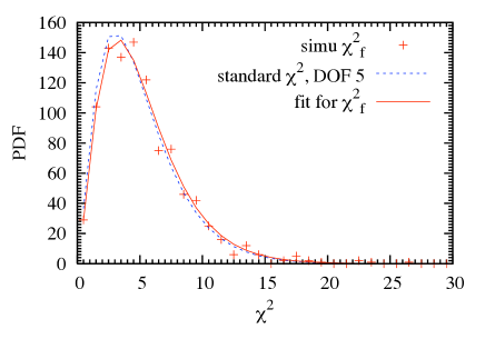
So far, we have quoted the $\Delta\chi^{2}$ values based on differences in mean peak counts between models. An important question is whether these $\Delta\chi^{2}$ can be interpreted as likelihoods, or confidence levels on parameter estimates. If the observables (in our case, the peak counts in each bin) were Gaussian distributed, and if they depended linearly on the the parameters (in our case, the cosmological parameters), then our $\Delta\chi^{2}$ would follow true $\chi^{2}$ distributions. When fitting a single parameter, as in our case above, $\Delta\chi^{2}=1,4,9$ would then correspond to the usual 68.3%, 95.4%, 99.7% confidence levels.

To see how good the above approximations are, in Fig. 9, we first show the distribution of $\chi^{2}_{f}(r)$ over different realizations in the fiducial model itself, shown by the red crosses (computed from Eq. (21), using noiseless, unscaled maps, and $z_{s}=2$). We fit these data with a standard chi-squared distribution $P_{\chi^{2}}(a\chi^{2},DOF)$, treating a linear scaling constant $a$ and the number of degrees of freedom DOF as free parameters. We find best-fit values of $a=1.0015$ and $DOF=5.23$. Reassuringly, the fit, shown by the red solid curve, is very good, with $a$ close to 1, and $DOF$ close to 5, the number of bins we used. For comparison, $P_{\chi^{2}}$ with $a=1$, $DOF=5$ is also shown as the blue dashed curve. Clearly, $\chi^{2}_{f}(r)$ closely follows a chi-squared distribution expected if the deviation of peak counts from the mean were Gaussian.

These results justify interpreting our $\Delta\chi^{2}$’s in the Tables above as (single-parameter) confidence levels. As seen in Table 5, the unscaled, noisy maps when $\sigma_{8}$ and $\Omega_{m}$ are varied correspond to “$2-2.5\sigma$” differences from the fiducial model; $w$ variations correspond to “$0.5-0.8\sigma$” differences.

IV.7 Impact of the Choice of Binning

In all our results above, we have used a fixed number of (five) bins, and performed only an ad-hoc optimization of the bin boundaries by hand. It is important to ask how our results are affected both by the number of bins, and by the placement of the bin boundaries. Ideally, one could use arbitrarily fine binning, and avoid such questions; in practice, we are limited by the finite number of realizations we can simulate.

Figure 10: $\Delta\chi^{2}$ from peak counts, as a function of the number of convergence bins. The fiducial model was compared to the low-$\sigma_{8}$, low-$\Omega_{m}$, and low-$w$ models, using noisy unscaled maps with $z_{s}=2$. Bin boundaries were chosen such that each bin contains equal counts, or such that “crossings” of the peak-count PDFs in a pair of cosmologies are avoided within bins (as labeled). The y-axis labels on the left refer to the $\sigma_{8}$ and $\Omega_{m}$ cases; the labels on the right to the $w$ case.

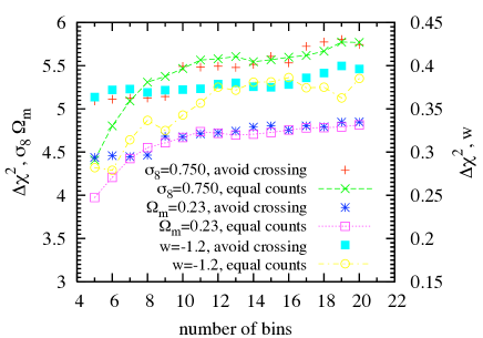
In Fig. 10, we show the $\Delta\chi^{2}$ in noisy unscaled maps, with $z_{s}=2$, between the fiducial model and the low-$\sigma_{8}$, low-$w$ and low-$\Omega_{m}$ models, as a function of the number of bins. We chose the bin boundaries either by following the approach of avoiding “crossings” of the peak-count PDFs in a pair of cosmologies within bins, or such that the mean number of peaks in each bin were the same. As the figure shows, the “avoid crossings” approach works quite well, and from 5 to 20 bins, the $\Delta\chi^{2}$’s increase only modestly (by $\approx 10\%$). The “equal counts” approach does more poorly (yielding smaller $\Delta\chi^{2}$) when the number of bins is small, but converges to a very similar values once the number of bins is $~{}\hbox to0.0pt{$>$\hss}{\lower 4.30554pt\hbox{$\sim$}}15$. These results give reassurance that we have a sufficient number of bins and the $\Delta\chi^{2}$’s shown in the Tables above have converged to within $\sim 10\%$.

In the next section, we vary multiple parameters simultaneously. In Figure 11, we show the marginalized errors of the three cosmological parameters $\sigma_{8}$, $\Omega_{m}$, $w$ from the combination of the peak counts and the power spectrum, as a function of the number of bins (in noisy unscaled maps, with $z_{s}=2$). When choosing the boundaries, we applied the “equal counts” approach for the peaks and the ”equally spaced” approach for the power spectrum. The details of computing the marginalized error is explained in the next section. The figure shows that the five bins are not sufficient in this case; however, the marginalized error converges to within $<10\%$ once the number of bins is $~{}\hbox to0.0pt{$>$\hss}{\lower 4.30554pt\hbox{$\sim$}}15$.

Figure 11: The marginalized errors of the three cosmological parameters $\sigma_{8}$, $\Omega_{m}$, $w$ from the combination of the peak counts and power spectrum, as a function of the number of convergence bins. The fiducial model was compared to the high/low-$\sigma_{8}$, high/low-$\Omega_{m}$, and high/low-$w$ models, using noisy unscaled maps with $z_{s}=2$. Bin boundaries were chosen such that each bin contains equal counts for peak counts and equally spaced with the cut at $\ell=20,000$ for the power spectrum. The y-axis labels on the left refer to the $\sigma_{8}$ and $\Omega_{m}$ cases; the labels on the right to the $w$ case.

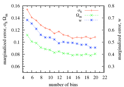
IV.8 Forecasting Marginalized Errors

marginalized error	$\sigma_{8}$	$w$	$\Omega_{m}$
z2	0.0065	0.030	0.0057
z1	0.0078	0.036	0.0057
z2+z1	0.0024	0.018	0.0022
Power Spectrum ($z_{s}=2$)	0.0047	0.026	0.0028
z2+Power Spectrum	0.0026	0.012	0.0019
z1+Power Spectrum	0.0037	0.020	0.0026
tomography combined	0.0012	0.0096	0.0010
combined/( z2+Power Spectrum)	0.47	0.79	0.52

Table 14: Marginalized 68% errors, in our noisy maps, on the cosmological parameters $\sigma_{8}$, $w$, and $\Omega_{m}$. In the top half of the table, peak counts and power spectra are considered separately. From top to bottom: (i) counts alone at $z_{s}=2$; (ii) counts alone at $z_{s}=1$; (iii) counts alone with both $z_{s}=1$ and $z_{s}=2$; (iv) power spectrum alone at $z_{s}=2$. In the bottom half of the table, counts and the power spectrum are combined. From top to bottom: (v) combining counts and power spectrum at $z_{s}=2$; (vi) combining counts and power spectrum at $z_{s}=1$; (vii) combining the above two cases to use all 4 observables – peak counts and power spectrum at $z_{s}=2$ and $z_{s}=1$; and finally (viii) the last combined results (row vii) divided by the “z2+Power Spectrum” results (row v). Each error quoted is marginalized over the other two parameters, and are scaled to a 20,000 $deg^{2}$ survey, such as LSST.

Figure 12: 68% percentile error ellipses in two-dimensional projections of the 3-dimensional parameter space of $\sigma_{8}$, $w$, and $\Omega_{m}$. In each panel, we show “tomography” results from noisy, unscaled maps for combining peak counts and power spectrum using either $z_{s}=2$, $z_{s}=1$, or their combination. The constraints are scaled to a 20,000 $deg^{2}$ survey, such as LSST.

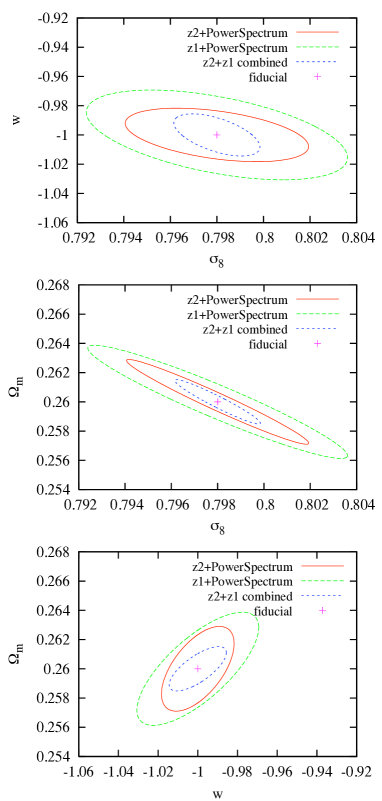
In all previous calculations, we have varied a single parameter, holding all the other parameters fixed. While this clarifies the raw cosmological sensitivity of the peak counts, justified if CMB (or other) observations can be used to determine the parameters with negligibly small errors, one has to simultaneously vary all uncertain parameter, and consider their degeneracies, to obtain realistic error forecasts (even in the limiting case of no systematic errors). While numerical limitations preclude us from exploring the full cosmological parameter space, we here use a Fisher matrix to obtain marginalized errors when the three parameters $\sigma_{8}$, $w$, and $\Omega_{m}$ are varied simultaneously. Degeneracies between these parameters are among the most important for both cluster counts (e.g. ref. HMH01 ) and for shear power spectra (e.g. ref. DCPFCSD ). We compute the marginalized errors from Eq. (22). We use the finite difference between the fiducial model and the low(high)-$\sigma_{8}$, low(high)-$w$ and low(high)-$\Omega_{m}$ models to estimate the backward(forward) derivatives with respect to these parameters. The average of backward and forward derivatives is used to calculate the Fisher matrix.

As mentioned above, we use 15 bins for the peak counts. The simple intuitive ad-hoc optimization of the bin boundaries, based on avoiding crossings in a single pair of cosmologies, which was used in the case of a single parameter, cannot be generalized in a straightforward way to the multi-parameter case. Indeed, we have found that when we use five bins, the results become sensitive to the choice of the cosmology pair over which the bin boundaries are optimized. Therefore we use the simpler (and unambiguous) scheme of equal-count bins; as shown in the previous section, the accuracy in this case convergences for $~{}\hbox to0.0pt{$>$\hss}{\lower 4.30554pt\hbox{$\sim$}}15$ bins. We emphasize that whenever there are significant degeneracies between parameters, the numerical accuracy requirements on the individual elements of the Fisher matrix become more stringent. on the individual elements of the Fisher matrix To validate our results, we have checked that our marginalized errors do converge when we use $~{}\hbox to0.0pt{$>$\hss}{\lower 4.30554pt\hbox{$\sim$}}15$ bins (see Fig. 11 above).

We found that, in addition to the binning, the marginalized errors for the peak counts, with a single source galaxy redshift, are sensitive to the direction of taking the finite-difference derivative (backward or forward). If we take any one of backward, forward and averaged derivatives for any of the parameters: $\sigma_{8}$, $w$, $\Omega_{m}$, among the marginalized errors of these 27 combinations, the marginalized errors for the three parameters vary by about $20\%-25\%$. On the other hand, the results become more stable when we combine the peak counts with the power spectrum (reducing the variations to $10\%-15\%$; to be consistent, we also use 15 bins for the power spectrum for computing marginalized errors). This behavior is consistent with the presence of strong degeneracies between parameters, which are broken when Fisher matrices corresponding to two or more observables are added (as shown for the combination of cluster counts and power spectra Wiley+04 ; FH07 ).

In Table 14, we show the results from combining peak counts and power spectrum in noisy, unscaled maps, using either $z_{s}=2$, $z_{s}=1$, or their combination. All the numbers in this table are scaled to the solid angle of $20,000~{}{\rm deg^{2}}$, representing an all-sky survey such as LSST. We simply divide our results from the $12~{}{\rm deg^{2}}$ maps by a factor $\sqrt{20,000/12}$ (see discussion in Paper I for this simple “extrapolation”). Comparing the individual peak-count (1st row) and power spectrum (4th row) errors at $z_{s}=2$ in the top half of the table with their combination (5th row), we see that the individual errors are roughly similar, considering the $20\%-25\%$ variation in the peak counts, whereas the combination improves on either by a factor of $\approx$two. As the table shows, combining the peak counts and power spectrum at $z_{s}=2$ yield 68% constraints as tight as $(\Delta\sigma_{8},\Delta\Omega_{m},\Delta w)=(0.0026,0.0012,0.019)$. Combining the peak counts and power spectrum at $z_{s}=1$ gives a constraints worse than at $z_{s}=2$, with $\Delta\sigma_{8}$ and $\Delta\Omega_{m}$ larger by $\sim 30\%$ and $\Delta w$ larger by $\sim 60\%$. This agrees with the previous $\Delta\chi^{2}$ results that $z_{s}=2$ generally yields a better sensitivity than $z_{s}=1$. We found that the marginalized errors from two redshifts together decrease significantly compared to the marginalized errors from $z_{s}=2$ alone. For the combination of the peak counts and the power spectrum, we found $\Delta\sigma_{8}$ and $\Delta\Omega_{m}$ are $\sim 50\%$ of the corresponding errors from $z_{s}=2$, $\Delta w$ is $\sim 75\%$ of the error from $z_{s}=2$. The large decrease of marginalized error from tomography is different from the results of $\Delta\chi^{2}$ of peak counts: tomography does $not$ significantly improve the sensitivity due to the correlation between two redshifts. This difference between $\Delta\chi^{2}$ (showing only raw cosmological sensitivity) and marginalized errors (showing also the degeneracy between cosmological parameters) clearly shows that the change in peak counts induced by each parameter has a different redshift-dependence. To be specific, the w-induced changes, as a function of redshift, cannot be degenerate with, for example, the Omega-induced changes (even if they can be very degenerate at a single redshift, blowing up the marginalized errors). Overall, these constraints are comparable to those expected from other forthcoming cosmology probes (see Paper I for a discussion), although a fair comparison would involve replicating the cosmological parameter set, and other assumptions made elsewhere, which is beyond the scope of this study.

Our results are also shown graphically in Fig. 12, which show the 68% joint two-parameter constraints (i.e., corresponding to $\Delta\chi^{2}=2.3$, and marginalized over the third parameter).

V Summary and Conclusions

In this paper, we used ray-tracing simulations, and a halo finder, to study the halo contributions to peaks present in convergence maps, expected in large forthcoming weak lensing surveys of the sky. This allowed us to understand the origin of relatively low-amplitude “$0.5-1.5\sigma$”, or “medium” peaks, and their sensitivity to cosmology. Our motivation to focus on these peaks is that they have been shown to drive the overall cosmology-sensitivity of the peak counts. Given that weak lensing by large scale structure is among the most promising cosmological datasets, expected to be available in the near future, the cosmological information content of these robustly measurable features must be understood.

We have found that unlike high peaks, which are typically produced and dominated by a single collapsed halo, the medium peaks are primarily caused by random noise. However, these medium peaks receive an important contribution from a projection of multiple (typically, 4-8) halos along the line of sight, which makes their number counts sensitive to cosmological parameters. We have shown that for source galaxies at high redshift ($z_{s}=2$) the presence of noise boosts the distinguishing power from peak counts – a counter-intuitive result that we have clarified analytically.

Our most important results are that the distribution of the medium peaks differ from similar-height peaks in a pure Gaussian random field (GRF). We have shown, explicitly, that the peaks contain cosmological information that differs from that in a GRF, and is non-degenerate with the power spectrum of the convergence. We have taken the first steps toward more realistic error forecasts, by obtaining the marginalized errors in the three–dimensional parameter space of $\sigma_{8}$, $w$, and $\Omega_{m}$. The results suggest that peak counts will play a significant role in tightening cosmological constraints from forthcoming large-solid-angle weak lensing surveys. On the other hand, we have not addressed here the long list of systematic errors that will ultimately limit the utility of convergence peaks. Given that the sensitivity relies heavily on peaks whose height is close to that of the expected noise, these issues will be especially important to address in future work. More generally, our results should motivate investigations to extract yet more cosmological information from nonlinear weak lensing features; Minkowski functionals appear to be a promising possibility MFs .