LOW-RANK DATA MODELING VIA THE MINIMUM DESCRIPTION LENGTH PRINCIPLE
Abstract
Robust low-rank matrix estimation is a topic of increasing interest, with promising applications in a variety of fields, from computer vision to data mining and recommender systems. Recent theoretical results establish the ability of such data models to recover the true underlying low-rank matrix when a large portion of the measured matrix is either missing or arbitrarily corrupted. However, if low rank is not a hypothesis about the true nature of the data, but a device for extracting regularity from it, no current guidelines exist for choosing the rank of the estimated matrix. In this work we address this problem by means of the Minimum Description Length (MDL) principle – a well established information-theoretic approach to statistical inference – as a guideline for selecting a model for the data at hand. We demonstrate the practical usefulness of our formal approach with results for complex background extraction in video sequences.
Index Terms— Low-rank matrix estimation, PCA, Robust PCA, MDL.
1 Introduction
The key to success in signal processing applications often depends on incorporating the right prior information about the data into the processing algorithms. In matrix estimation, low-rank is an all-time popular choice, with analysis tools such as Principal Component Analysis (PCA) dominating the field. However, PCA estimation is known to be non-robust, and developing robust alternatives is an active research field (see [1] for a review on low-rank matrix estimation). In this work, we focus on a recent robust variant of PCA, coined RPCA [1], which assumes that the difference between the observed matrix , and the true underlying data , is a sparse matrix whose non-zero entries are arbitrarily valued. It has been shown in [1] that (alternatively, ) can be recovered exactly by means of a convex optimization problem involving the rank of and the norm of . The power of this approach has been recently demonstrated in a variety of applications, mainly computer vision (see [2] and http://perception.csl.uiuc.edu/matrix-rank/applications.html for examples).
However, when used as a pure data modeling tool, with no assumed “true” underlying signal, the rank of in a PCA/RPCA decomposition is a parameter to be tuned in order to achieve some desired goal. A typical case is model selection [3, Chapter 7], where one wants to select the size of the model (in this case, rank of the approximation) in order to strike an optimal balance between the ability of the estimated model to generalize to new samples, and its ability to adapt itself to the observed data (the classic overfitting/underfitting trade-off in statistics). The main issue in model selection is how to formulate this balance as a cost function.
In this work, we address this issue via the Minimum Description Length (MDL) principle [4, 5].111While here we address the matrix formulation, the developed framework is applicable in general, including to sparse models, and such general formulation will be reported in our extended version of this work. MDL is a general methodology for assessing the ability of statistical models to capture regularity from data. The MDL principle can be regarded as a practical implementation of the Occam’s razor principle, which states that, given two descriptions for a given phenomenon, the shorter one is usually the best. In a nutshell, MDL equates “ability to capture regularity” with “ability to compress” the data, using codelength or compressibility as the metric for measuring candidate models.
The resulting framework provides a robust, parameter-free low-rank matrix selection algorithm, capable of capturing relevant low-rank information in the data, as in the video sequences from surveillance cameras in the illustrative application here reported. From a theoretical standpoint, this brings a new, information theoretical perspective into the problem of low-rank matrix completion. Another important feature of an MDL-based framework such as the one here presented is that new prior information can be naturally and easily incorporated into the problem, and its effect can be assessed objectively in terms of the different codelengths obtained.
2 Low-rank matrix estimation/approximation
Under the low-rank assumption, a matrix can be written as , where and , where is some matrix norm. Classic PCA provides the best rank- approximation to under the assumption that is a random matrix with zero-mean IID Gaussian entries,
| (1) |
However, PCA is known to be non-robust, meaning that the estimate can vary significantly if only a few coefficients in are modified. This work, providing an example of introducing the MDL framework in this type of problems, focuses on a robust variant of PCA, RPCA, introduced in [1]. RPCA estimates via the following convex optimization problem,
| (2) |
where is the nuclear norm of ( denotes the -th singular value of ). The rationale behind (2) is as follows. First, the fitting term allows for large errors to occur in the approximation. In this sense, it is a robust alternative to the norm used in PCA. The second term, is a convex approximation to the PCA constraint , merged into the cost function via a Lagrange multiplier .
This formulation has been recently shown to be notoriously robust, in the sense that, if a true low-rank matrix exists, it can be recovered using (2) even when a significant amount of coefficients in are arbitrarily large [1]. This can be achieved by setting , so that the procedure is parameter-free.
2.1 Low-rank approximation as dimensionality reduction
In many applications, the goal of low-rank approximation is not to find a “true” underlying matrix , but to perform what is known as “dimensionality reduction,” that is, to obtain a succinct representation of in a lower dimensional subspace. A typical example is feature selection for classification. In such cases, is not necessarily a small measurement perturbation, but a systematic, possibly large, error derived from the approximation process itself. Thus, RPCA arises as an appealing alternative for low-rank approximation.
However, in the absence of a true underlying signal (and deviation ), it is not clear how to choose a value of that produces a good approximation of the given data for a given application. A typical approach would involve some cross-validation step to select to maximize the final results of the application (for example, minimize the error rate in a classification problem).
The issue with cross-validation in this situation is that the best model is selected indirectly in terms of the final results, which can depend in unexpected ways on later stages in the data processing chain of the application (for example, on some post-processing of the extracted features). Instead, we propose to select the best low-rank approximation by means of a direct measure on the intrinsic ability of the resulting model to capture the desired regularity from the data, this also providing a better understanding of the actual structure of the data. To this end, we use the MDL principle, a general information-theoretic framework for model selection which provides means to define such a direct measure.
3 MDL-based low-rank model selection
Consider a family of candidate models which can be used to describe a matrix exactly (that is, losslessly) using some encoding procedure. Denote by the description length, in bits, of under the description provided by a given model . MDL will then select the model for for which is minimal, that is . It is a standard practice in MDL to use the ideal Shannon code for translating probabilities into codelengths. Under this scheme, a sample value with probability is assigned a code with length (all logarithms are taken on base ). This is called an ideal code because it only specifies a codelength, not a specific binary code, and because the codelengths produced can be fractional.
By means of the Shannon code assignment, encoding schemes can be defined naturally in terms of probability models . Therefore, the art of applying MDL lies in defining appropriate probability assignments , that exploit as much prior information as possible about the data at hand, in order to maximize compressibility. In our case, there are two main components to exploit. One is the low-rank nature of the approximation , and the other is that most of the entries in will be small, or even zero (in which case will be sparse). Given a low-rank approximation of , we describe as the pair , with . Thus, our family of models is given by . As , we index solely by . With these definitions, the description codelength of is given by . Now, to exploit the low rank of , we describe it in terms of its reduced SVD decomposition,
| (3) |
where is the rank of (the zero-eigenvalues and the respective left and right eigenvectors are discarded in this description). We now have . Clearly, such description will be short if is significantly smaller than . We may also be able to exploit further structure in , and .
3.1 Encoding
The diagonal of is a non-increasing sequence of positive values. However, no safe assumption can be made about the magnitude of such values. For this scenario we propose to use the universal prior for integers, a general scheme for encoding arbitrary positive integers in an efficient way [6],
| (4) |
where the sum stops at the first non-positive summand, and is added to satisfy Kraft’s inequality (a requirement for the code to be uniquely decodable, see [7, Chapter 5]). In order to apply (4), the diagonal of , , is mapped to an integer sequence via , where denotes rounding to nearest integer (this is equivalent to quantizing with precision ).
3.2 Encoding U and V, general case
By virtue of the SVD algorithm, the columns of and have unit norm. Therefore, the most general assumption we can make about and is that their columns lie on the respective -dimensional and -dimensional unit spheres.
An efficient code for this case can be obtained by encoding each column of and in the following manner. Let be a column of ( is similarly encoded). Since is assumed to be distributed uniformly over the -dimensional unit sphere, the marginal cumulative density function of the first element , , corresponds to the proportion of vectors that lie on the unit spherical cap of height (see Figure 1(a)). This proportion is given by where and are the area of spherical cap of height and the total surface area of the -dimensional sphere of radius respectively. These are given for the case () by (see [8]),
where , and are the regularized incomplete Beta function and the Beta function of parameters respectively, and is the Gamma function. When we simply have . For encoding we have so that
| (5) |
since . Finally, we compute the Shannon codelength for as
where in we applied the Fundamental Theorem of Calculus to the definition of and the chain rule for derivatives.
With encoded, the vector is uniformly distributed on the surface of the -dimensional sphere of radius , and we can apply the same formula to compute the probability of , .

Finally, to encode the next column , we can exploit its orthogonality with respect to the previous ones and encode it as a vector distributed uniformly over the dimensional sphere corresponding to the intersection of the unit sphere and the subspace perpendicular to .
In order to produce finite descriptions and , both and also need to be quantized. We choose the quantization steps for and adaptively, using as a starting point the empirical standard deviation of a normalized vector, that is, and respectively, and halving these values until no further decrease in the overall codelength is observed.
3.3 Encoding U predictively
If more prior information about and is available, it should be used as well. For example, in the case of our example application, the columns of are consecutive frames of a video surveillance camera. In this case, the columns of represent “eigen-frames” of the video sequence, while contains information about the evolution in time of those frames (this is clearly observed in figures 2 and 3). Therefore, the columns of can be assumed to be piecewise smooth, just as normal static images are. To exploit this smoothness, we apply a predictive coding to the columns of . Concretely, to encode the -th column of , we reshape it as an image of the same size as the original frames in . We then apply a causal bilinear predictor to produce an estimate of , where , assuming out-of-range pixels to be . The prediction residual is then encoded in raster scan as a sequence of Laplacian random variables with unknown parameter . This encoding procedure, common in predictive coding, is depicted in Figure 1(b).
Since the parameters are unknown, we need to encode them as well to produce a complete description of . In MDL, this is done using the so-called universal encoding schemes, which can be regarded as a generalization of classical Shannon encoding to the case of distributions with unknown parameters (see [5] for a review on the subject). In this work we adopt the so-called universal two-part codes, and apply it to encode each column separately. Under this scheme, the unknown Laplacian parameter for is estimated via Maximum Likelihood, , and quantized with precision , thus requiring bits. Given the quantized , is described using the discretized Laplacian distribution . Here and are constants which can be disregarded for optimization purposes. It was shown in [4] that the precision asymptotically yields the shortest two-parts codelength.
3.4 Encoding V predictively
We also expect a significant redundancy in the time dimension, so that the columns of are also smooth functions of time (in this case, sample index ). In this case, we apply a first order causal predictive model to the columns of , by encoding them as sequences of prediction residuals, , with for and . Each predicted column is encoded as a sequence of Laplacian random variables with unknown parameter . As with , we use a two-parts code here to describe the data and the unknown Laplacian parameters together. This time, since the length of the columns is , the codelength associated to each is .
3.5 Encoding E
We exploit the (potential) sparsity of by first describing the indexes of its non-zero locations using an efficient universal two-parts code for Bernoulli sequences known as Enumerative Code [9], and then the non-zero values at those locations using a Laplacian model. In the specific case of the experiments of Section 4, we encode each row of separately. Because each row of corresponds to the pixel values at a fixed location across different frames, we expect some of these locations to be better predicted than others (for example, locations which are not occluded by people during the sequences), so that the variance of the error (hence the Laplacian parameter) will vary significantly from row to row. As before, the unknown parameters here are dealt with using a two-parts coding scheme.
3.6 Model selection algorithm
To obtain the family of models corresponding to all possible low-rank approximations of , we apply the RPCA decomposition (2) for a decreasing sequence of values of , obtaining a corresponding sequence of decompositions . We obtain such sequence efficiently by solving (2) via a simple modification of the Augmented Lagrangian-based (ALM) algorithm proposed in [10] to allow for warm restarts, that is, where the initial ALM iterate for computing is . We then select the pair , .
4 Results and conclusion
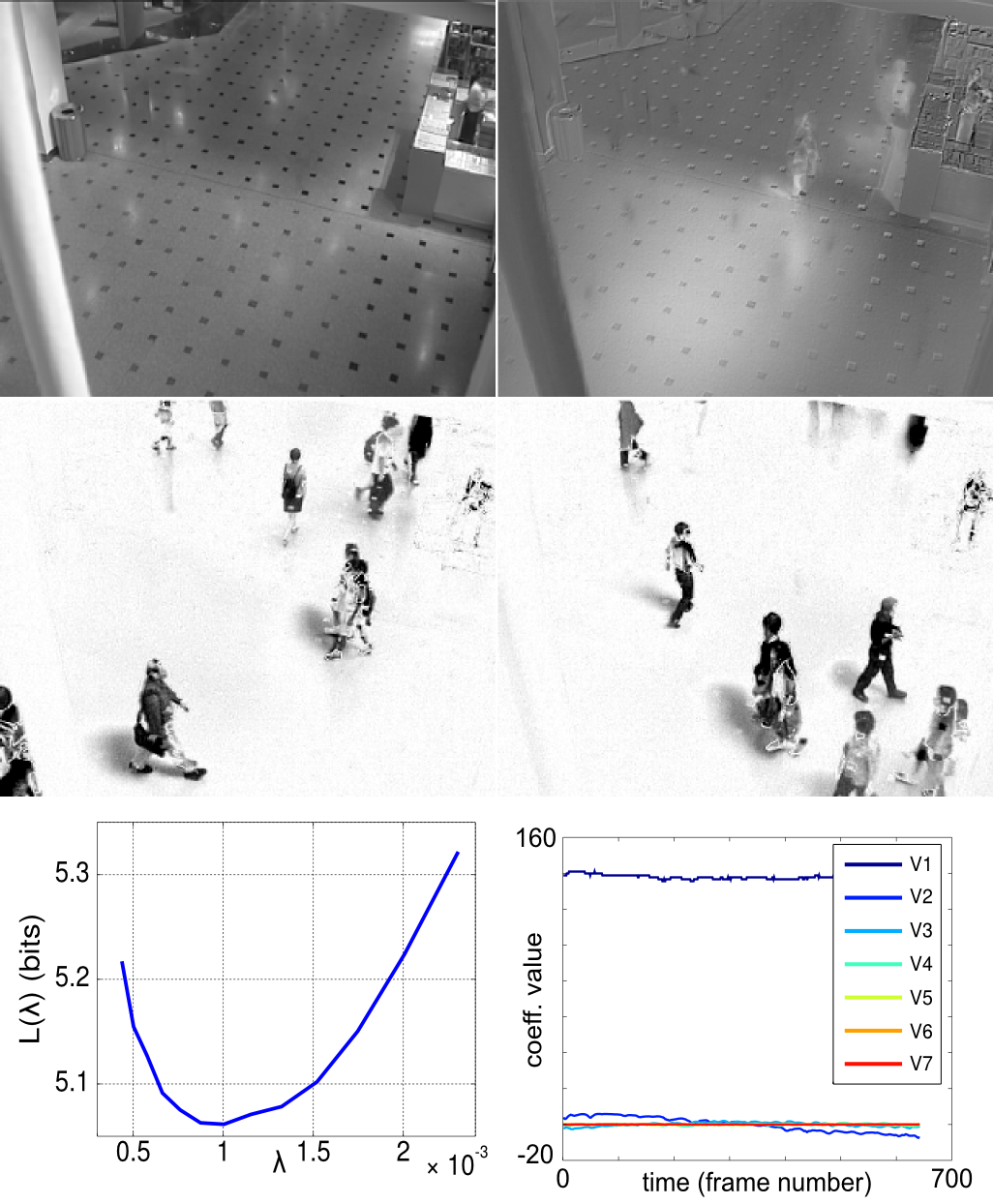
In order to have a reference base, we repeated the experiments performed in [2] using our algorithm. These experiments consist of frames from surveillance cameras which look at a fixed point where people pass by. The idea is that, if frames are stacked as columns of , the background can be well modeled as a low-rank component of (), while the people passing by appear as “spurious errors” (). Clearly, if the background in all frames is the same, it can be very well modeled as a rank- matrix where all the columns are equal. However, lighting changes, shadows, and reflections, “raise” the rank of the background, and the appropriate rank needed to model the background is no longer obvious.
Concretely, the experiments here described correspond to two sequences: “Lobby” and “ShoppingMall,” whose corresponding results are summarized respectively in figures 2 and 3.222The full videos can be viewed at http://www.tc.umn.edu/~nacho/lowrank/. At the top of both figures, the first two left-eigenvectors and of are shown as 2D images. The middle shows two sample frames of the error approximation. The -vs- curve is shown at the bottom-left (note that the best is not the one dictated by the theory in [1], which are for Lobby and for ShoppingMall, both outside of the plotted range), and the scaled right-eigenvectors are shown on the bottom-right. In both cases, the resulting decomposition recovered the low-rank structure correctly, including the background, its changes in illumination, and the effect of shadows. It can be appreciated in the figures 2-3 how such approximations are naturally obtained as combinations of a few significant eigen-vectors, starting with the average background, followed by other details.
4.1 Conclusion
In summary, we have presented an MDL-based framework for low-rank data approximation, which combines state-of-the-art algorithms for robust low-rank decomposition with tools from information theory. This framework is able to capture the underlying low-rank information on the experiments that we performed, out of the box, and without any hand parameter tuning, thus constituting a promising competitive alternative for automatic data analysis and feature extraction.

References
- [1] E. Candès, X. Li, Y. Ma, and J. Wright, “Robust principal component analysis?,” Journal of the ACM, vol. 58, no. 3, May 2011.
- [2] J. Wright, A. Ganesh, S. Rao, Y. Peng, and Y. Ma, “Robust principal component analysis: Exact recovery of corrupted low-rank matrices by convex optimization,” in Adv. NIPS, Dec. 2009.
- [3] T. Hastie, R. Tibshirani, and J. Friedman, The Elements of Statistical Learning: Data Mining, Inference and Prediction, Springer, 2nd edition, Feb. 2009.
- [4] J. Rissanen, “Modeling by shortest data description,” Automatica, vol. 14, pp. 465–471, 1978.
- [5] A. Barron, J. Rissanen, and B. Yu, “The minimum description length principle in coding and modeling,” IEEE Trans. IT, vol. 44, no. 6, pp. 2743–2760, 1998.
- [6] J. Rissanen, Stochastic Complexity in Statistical Inquiry, Singapore: World Scientific, 1992.
- [7] T. Cover and J. Thomas, Elements of Information Theory, John Wiley and Sons, Inc., 2 edition, 2006.
- [8] S. Li, “Concise formulas for the area and volume of a hyperspherical cap,” Asian J. Math. Stat., vol. 4, pp. 66–70, 2011.
- [9] T. M. Cover, “Enumerative source encoding,” IEEE Trans. IT, vol. 19, no. 1, pp. 73–77, 1973.
- [10] Z. Lin, M. Chen, and Y. Ma, “The Augmented Lagrange Multiplier Method for exact recovery of corrupted low-rank matrices,” http://arxiv.org/abs/1009.5055.