Dipole Showers and Automated NLO Matching in Herwig++

Abstract

We report on the implementation of a coherent dipole shower algorithm along with an automated implementation for dipole subtraction and for performing powheg- and MC@NLO-type matching to next-to-leading order (NLO) calculations. Both programs are implemented as add-on modules to the event generator Herwig++. A preliminary tune of parameters to data acquired at LEP, HERA and Drell-Yan pair production at the Tevatron has been performed, and we find an overall very good description which is slightly improved by the NLO matching.

1 Introduction

Many physics analyses at the Large Hadron Collider (LHC) are nowadays based on Monte Carlo simulations Bahr:2008pv ; Corcella:2002jc ; Sjostrand:2007gs ; Sjostrand:2006za ; Gleisberg:2008ta , e.g. for acceptance determination or even for background subtraction. With the high precision aimed for in many analyses it is mandatory to provide many of the simulations with the highest possible theoretical accuracy. For most processes this is now next-to-leading order (NLO) in the perturbative expansion of Quantum Chromodynamics (QCD). During the last decade, enormous progress was made in the development of techniques to match NLO calculations on the one hand and to merge multiple jet tree level matrix elements on the other hand with parton shower algorithms.

First attempts to improve parton shower emission patterns with the information from the full matrix element for the hardest gluon emission were made with so-called matrix element corrections Seymour:1994df ; Norrbin:2000uu , that have long been implemented in the standard event generators. The next big improvement was made when matrix elements for multiple hard emissions were merged with parton shower algorithms, first for $e^{+}e^{-}$ annihilation processes Catani:2001cc ; Lonnblad:2001iq and then also for hadronic collisions Krauss:2002up . An alternative approach was proposed in Hoche:2006ph , where different implementations have been systematically compared as well. The experience that was made with these algorithms over the last years Lavesson:2007uu has lead to further improvements Hoeche:2009rj ; Hamilton:2009ne such that now the systematic uncertainties due to e.g. matching scale dependence have been significantly reduced.

Matching to NLO matrix elements has been initiated first with a phase space slicing method Potter:2000an ; Potter:2001ej ; Dobbs:2001dq . A more systematic matching has then been introduced by Frixione and Webber in the MC@NLO approach Frixione:2002ik . This approach has then been generalised to include massive partons Frixione:2003ei . Many processes have been included in the meantime Frixione:2005vw ; Frixione:2007zp ; Frixione:2008yi . As the algorithm depends on subtraction terms for a specific parton shower implementation, the first versions of MC@NLO have been tailored to work with Herwig only. Now, it also works with Herwig++, i.e. as the subtraction scheme has been generalised towards the Herwig++ parton shower implementation, all processes available in the MC@NLO package can also be showered with Herwig++ to achieve formal accuracy at NLO Frixione:2010ra .

As the matching of NLO matrix elements and parton shower algorithms takes place perturbatively to the specified order, i.e. the next-to-leading order, there is formally an ambiguity left that can be used to devise alternative matching schemes. One such scheme has been proposed by Nason Nason:2004rx and now goes under the name powheg. The guiding principle of this algorithm is to allow for a matching algorithm that does not introduce events with negative weight, as the MC@NLO prescription does. This approach has also been very successfully established during the last years and implemented as a separate program package Frixione:2007nu . Many processes are available in this program package Nason:2006hfa ; Frixione:2007nw ; Alioli:2008gx ; Alioli:2008tz ; Alioli:2010xa . However, the method itself is also used by other groups to match NLO calculations with parton showers within a given shower package. Many processes are available with Herwig++ Hamilton:2008pd ; Hamilton:2009za ; Hamilton:2010mb ; D'Errico:2011um ; D'Errico:2011sd or sherpa Hoche:2010pf . The internal implementations benefit from the inclusion of truncated showers (see below).

On the parton shower side, a number of new parton shower algorithms have been developed during the last years, partly together with the rewrite of old generators Gieseke:2003rz ; Sjostrand:2004ef . Many new developments have addressed the idea of implementing a shower that is directly related to the subtraction terms commonly used in NLO calculations. This led to the implementation of parton showers with splitting kernels based on the Catani–Seymour subtraction scheme Catani:1996vz ; Catani:2002hc for NLO calculations Schumann:2007mg ; Dinsdale:2007mf , which was proposed in Nagy:2005aa . Similar ideas are followed with other subtraction schemes as e.g. in the vincia shower Giele:2007di where QCD antenna subtraction terms are facilitated.

With more and more NLO calculations being matched one-by-one the question arises whether this step can be automated. In fact, the powheg method is already a first step into this direction, as the method as such is independent of the showering algorithm. In particular, no specific subtraction terms or the like are needed in order to match a given NLO calculation to any shower. There are subtleties on the shower side, though. The powheg method guarantees to give the hardest emission within the parton evolution and ensures that this is generated according to the phase space weighting of the NLO matrix element. However, if the shower does not evolve in the same hardness measure as the powheg algorithm, one has to introduce so-called truncated showers. This has been discussed already in early powheg implementations LatundeDada:2006gx and is now part of Herwig++ Hamilton:2009ne and sherpa Hoeche:2009rj .

Many NLO calculations are available as ready-to-use computer codes that often come as packages that include a number of processes at NLO already. Most of these codes use the Catani–Seymour subtraction method to regularise infrared divergences. More recently, also the complete automation of NLO calculations has been discussed with first tools readily available vanHameren:2009dr ; Hirschi:2011pa , based on the approach Ossola:2007ax . Some more calculations are already based on a fully automated tool chain Berger:2009zg ; Berger:2010zx ; Giele:2008bc ; Mastrolia:2010nb ; Heinrich:2010ax . Part of this progress relies on the automatic generation of Catani–Seymour subtraction terms Gleisberg:2007md ; Hasegawa:2009tx ; Frederix:2010cj or FKS subtraction terms Frederix:2009yq . The latest developments unify the matching of multiple tree–level emissions and the matching of NLO corrections to the Born level Hamilton:2010wh ; Hoche:2010kg .

In this paper we introduce an implementation of a parton shower based on the Catani–Seymour subtraction terms, similar to the showers introduced in Schumann:2007mg ; Dinsdale:2007mf . The goal of the implementation is to provide a framework for an automatic matching of NLO computations to a parton shower. The use of the subtraction terms is highly beneficial as the MC@NLO like matching, that is based on a subtraction of the parton shower contribution to the NLO observable becomes trivial. Together with a framework to handle powheg like matching we will have the possibility to check systematics within a single implementation. By using a shower based framework we may directly make use of truncated showers in order to minimise systematic uncertainties inherent to the matching formalism. As a first step in this programme we present the shower implementation, which is embedded as a module in the Herwig++ event generator. In addition we present NLO matchings to the basic QCD processes.

The paper is organised as follows. In Sec. 2 we introduce the dipole shower in detail. Sec. 3 introduces the implementation of an automatic matching with this parton shower, that we call Matchbox. In Secs. 4, 5 and 6 we present comparisons to data from LEP, HERA and the Tevatron, respectively.

2 Dipole Showers

The dipole shower algorithm outlined in Platzer:2009jq has been implemented as an add-on module to Herwig++, Bahr:2008pv . In this section we briefly review its properties and give a full description of the implementation.

The authors have shown that parton showers based on Catani-Seymour subtraction kernels Catani:1996vz correctly reproduce the Sudakov anomalous dimensions and properly include effects of soft gluon coherence, upon using an ordering of emissions in transverse momenta as defined by the emitting dipoles. The simple inversion of the kinematic parametrisation used in the context of NLO subtraction, however, does not resemble a physical picture for initial state radiation. An alternative has been suggested and implemented in the simulation presented here.

2.1 Starting the Shower

The dipole shower starts evolving off a hard sub process, which is assigned colour flow information in the large-$N_{c}$ limit. This colour flow information is used to first sort all coloured partons attached to the hard sub process into colour singlets. Practically, this is done by making use of the fact that a colour singlet is ‘simply connected’ in the sense of its colour flow topology: Any parton $i$ in a colour singlet can be reached from a parton $j$ in the same singlet by just following colour lines and changing from a colour to an anti-colour line at an external gluon. Each colour singlet is now an independently evolving entity, and can only split into two colour singlets in the presence of a $g\to q\bar{q}$ splitting. In the next step, the partons in each singlet are sorted such that colour connected partons are located at neighbouring positions, when representing the singlet group of partons as a sequence. Note that these sequences may be open or closed: We will call a sequence open, or non-circular, if there exists a circular permutation of the elements in it such that the partons at the first and last position are not colour connected. Conversely, if there does not exist such a permutation, the sequence is called circular or closed. The possible sequences are depicted in Fig. 1. Once this sorting has been accomplished, we will refer to these singlet sequences as dipole chains: each pair of subsequent partons in a singlet sequence forms a dipole, which may radiate. For each parton in each dipole, a hard scale is then determined as defined in Platzer:2009jq .

2.2 Evolution of the Parton Ensemble

The main shower algorithm acts on a set of dipole chains, and proceeds as long as this set is not empty. Dipole chains are removed from the list, if they stopped evolving, i.e. if there was no splitting selected with a $p_{\perp}^{2}$ above the shower’s infrared cutoff $\mu_{IR}^{2}$. The first entry in the set of dipole chains is taken to be the current chain. For each dipole $(i,j)$ in the current chain (with both possible emitter–spectator assignments, i.e. also considering $(j,i)$ along with $(i,j)$), any possible splitting $(i,j)\to(i^{\prime},k,j)$ is considered to compete with all other possible splittings of the chain. For any such splitting, given a hard scale $p_{\perp}^{2}$ associated to the emitter under consideration, a scale $q_{\perp}^{2}$ is selected with probability given by the Sudakov form factor

$$\Delta_{(i,j)\to(i^{\prime},k,j)}(q_{\perp}^{2},p_{\perp}^{2})=\\ \exp\left(-\int_{q_{\perp}^{2}}^{p_{\perp}^{2}}{\rm d}q^{2}\int_{z_{-}(q^{2})}^{z_{+}(q^{2})}{\rm d}zP_{(i,j)\to(i^{\prime},k,j)}(q^{2},z)\right)\ ,$$ (1)

where $P_{(i,j)\to(i^{\prime},k,j)}(q^{2},z)$ is the appropriate splitting probability as defined in Platzer:2009jq , using the respective dipole splitting function $V_{i^{\prime},k;j}$.

The splitting with the largest selected value of $q_{\perp}^{2}$ is then chosen to be the one to happen, except the largest $q_{\perp}^{2}$ turned out to be below the infrared cutoff. In this case the current chain is removed from the set of dipole chains, inserted into the event record and the algorithm proceeds with the next chain. The momentum fraction $z$ is chosen to be distributed according to ${\rm d}P_{(i,j)\to(i^{\prime},k,j)}(q_{\perp}^{2},z)$. Since for now we use azimuthally averaged splitting kernels, the azimuthal orientation of the transverse momentum is chosen to be distributed flat. The momenta of the splitting products and the spectator after emission are then calculated as specified in Platzer:2009jq .

As the evolution factors into dipole chains as independently evolving objects, all possible emitters in the chain – after having inserted the generated splitting – now get the selected $q_{\perp}^{2}$ assigned as their hard scale, or stay at the kinematically allowed scale $p_{\perp,i,j}^{2}$ if $q_{\perp}^{2}>p_{\perp,i,j}^{2}$. If a $g\to q\bar{q}$ splitting has been selected for a circular chain, this chain becomes non-circular. If it has been selected for an already non-circular chain, this chain breaks up into two independent chains exactly between the $q\bar{q}$-pair, owing to the colour structure of this splitting. This situation, along with non-exceptional splittings is depicted in Fig. 1.

$\to$

$\to$

Gluon emission off a circular chain.

The chain stays circular.

$\to$

$\to$

Gluon emission off a non-circular chain.

The chain stays non-circular.

$\to$

$\to$

$g\to q\bar{q}$ splitting in a circular chain.

The chain becomes non-circular.

$\to$

$\to$

$g\to q\bar{q}$ splitting in a non-circular chain,

triggering breakup of the chain.

Figure 1: Examples of parton emission from dipole chains. In these examples always the upper dipole has been considered for emissions. Note that any dipole may split in two different ways, splitting either of its legs. These competing possibilities are not shown in the transition diagrams.

2.3 Finishing the Shower

After the shower evolution has terminated, the incoming partons with momenta $p_{a,b}$ in general have non-vanishing transverse momenta with respect to the beam directions. This necessitates a realignment of the complete event encountered at this stage. Following the arguments of Platzer:2009jq , the momenta of the evolved incoming partons $p_{a,b}$ are taken to define the frame of the collision at hand, i.e. hadron momenta $\tilde{P}_{a,b}$. We then seek a Lorentz transformation to take $\tilde{P}_{a,b}$ to the externally fixed hadron momenta $P_{a,b}$, which is in turn used to realign the complete event.

To construct the momenta of the incoming hadrons $\tilde{P}_{a,b}$, we require the three-momenta of $\tilde{P}_{a,b}$ being collinear with the respective partonic three-momenta and define momentum fractions

$$x_{a,b}=\frac{2\tilde{P}_{b,a}\cdot p_{a,b}}{S}\ .$$ (2)

The momentum fractions are further constrained by requiring that

$$(\tilde{P}_{a}+\tilde{P}_{b})^{2}=S$$ (3)

where $S$ is the centre-of-mass energy squared of the collision, such that the desired Lorentz transformation exists.

The second constraint is in principle to be chosen in such a way as to preserve the most relevant kinematic quantity of the hard process which initiated the showering. By default, we choose this to be the rapidity of a system $X$, which is either the system of non-coloured particles at the hard sub-process, or the complete final state in case of a pure QCD hard scattering.

2.4 Cluster Hadronization

The cluster hadronization model, originally proposed in Webber:1983if , is the hadronization model used by the Herwig++ event generator. The model in its initial stage just after parton showering, performs a splitting of gluons into quark-antiquark pairs such that in the large-$N_{c}$ limit a set of colour singlet clusters emerge from the event under consideration.

These clusters are then subsequently converted into hadrons, by either splitting them into clusters of lower invariant mass or performing directly the decay to meson pairs, in case another $q\bar{q}$ pair is ‘popped’ from the vacuum inside the cluster, or baryon pairs, where the creation of a diquark-antidiquark pair is assumed. Further details of the model will not be discussed here.

The main assumption of the model is however, that both quarks are located on their constituent mass shell, and gluons are as well assigned a non-vanishing constituent mass, entering as a parameter of the model. In the standard Herwig++ parton shower, acting as a $1\to 2$ cascade, only scales and momentum fractions of the splittings are determined during the evolution, the full kinematic information being constructed after the end of the perturbative evolution. This setup thus straightforwardly allows to include the constituent masses in this particular step. Since the dipole shower preserves momentum conservation locally to each splitting, ending up with a set of massless partons, such a treatment is not possible.

The way to perform the ‘reshuffling’ of the massless parton momenta to their constituent mass shells is chosen to be the following algorithm: Let $Q_{c}$ be the total momentum of all final state partons and perform a boost $\Lambda_{c}$ to the centre-of-mass system of $Q_{c}$, $\Lambda_{c}Q_{c}=(\hat{Q}_{c},{\mathbf{0}})$. The boosted parton momenta $p_{i}$ are now put on the constituent mass shell, including a global rescaling of their three-momenta,

$$p_{i}=\left(|{\mathbf{p}}_{i}|,{\mathbf{p}}_{i}\right)\to p^{\prime}_{i}=\left(\sqrt{\xi^{2}|{\mathbf{p}}_{i}|^{2}+m_{c,i}^{2}},\xi{\mathbf{p}}_{i}\right)\ .$$ (4)

Momentum conservation then implies the following relation be satisfied,

$$\hat{Q}_{c}=\sum_{i}\sqrt{\xi^{2}|{\mathbf{p}}_{i}|^{2}+m_{c,i}^{2}}\ ,$$ (5)

which may be solved numerically to yield a value for $\xi$. Finally the inverse boost $\Lambda_{c}^{-1}$ is applied to the new parton momenta $p^{\prime}_{i}$.

3 The Matchbox Implementation

Closely related to the dipole shower implementation, though technically independent of it, is the development of the Matchbox module. Matchbox is based on an extended version of ThePEG, the extensions providing functionality to perform hard process generation at the level of NLO QCD accuracy and easing the setup of run time interfaces to external codes for hard process generation. We have implemented an automated generation of subtraction terms based on the dipole subtraction formalism Catani:1996vz , based on the information available from ThePEG matrix element implementations, which will be discussed in further detail in section 3.2. A full NLO calculation to be run in the Matchbox framework only requires the implementation of tree-level and one-loop amplitudes, the presence of colour (and spin) correlated amplitudes for the Born process and the presence of a phase space generator appropriate to the process under consideration. Fig. 2 sketches the involved software modules and their interaction with an external implementation of a NLO calculation.

Figure 2: A sketch of the interaction of the Matchbox and dipole shower modules as integrated in Herwig++. To perform a matched NLO calculation an external code only has to provide tree-level and one-loop amplitudes along with colour- and spin-correlated amplitudes of the Born process and an appropriate phase space generator.

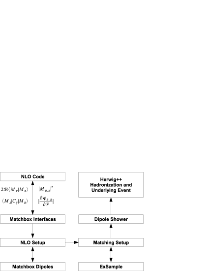
Besides being capable of performing a Monte Carlo integration of ‘plain’ NLO corrections, the main purpose of Matchbox is to turn a NLO calculation into a matched calculation to be consistently combined with a parton shower. Here, functionality is especially provided to calculate the inclusive NLO cross section differential in the Born degrees of freedom, which, along with a matrix element correction to the shower, is the main ingredient to the powheg method of combining parton showers and NLO QCD corrections.

Matchbox is automatically generating matrix element corrections from the NLO real emission contribution. It further allows the possibility to overcome problems in the powheg matching owing to radiation zeroes in the Born matrix element. The matrix element correction splitting kernel, which is essentially defined by the ratio of real emission and Born matrix elements squared is turned into the corresponding distribution including the Sudakov form factor by using the ExSample library, Platzer:2011dr . ExSample allows the efficient sampling of distributions of this type, without having to provide any analytic knowledge on the splitting kernel or trying to estimate enhancement factors to simpler functions such as dipole splitting kernels. ExSample is also used to sample emissions in the dipole shower implementation.

3.1 Notation

We consider NLO calculations carried out using the dipole subtraction method, Catani:1996vz . Instead of using the notation established there, we unify the indices of all possible dipoles to ease readability, as expressions become quite complicated especially when considering the powheg type matching. For the subtraction dipoles we choose the notation

$${\cal D}_{ij,k}\ ,{\cal D}_{ij}^{a}\ ,{\cal D}_{k}^{ai}\ ,{\cal D}^{ai,b}\quad\to\quad{\cal D}_{\alpha}\ ,$$ (6)

where the arguments are unified and we make explicit the dependence on either real emission or ‘tilde’ kinematics, e.g.

$${\cal D}_{ij,k}(q_{a},q_{b};q_{1},...,q_{n+1})\quad\to\quad{\cal D}_{\alpha}(p_{n}^{\alpha}(q_{n+1})|q_{n+1})\ .$$ (7)

In this notation, $p_{n}$ now refers to the whole phase space point,

$$p_{a},p_{b};p_{1},...,p_{n}\quad\to\quad p_{n}\equiv(\hat{p}_{a},\hat{p}_{b};\hat{p}_{1},...,\hat{p}_{n})\ ,$$ (8)

where we have added hat symbols to the momenta to distinguish a single momentum from a complete phase space point. The ‘tilde’ mapping and its inverse are denoted by

$$\widetilde{p_{ij}}(q_{i},q_{j},q_{k})\ ,\widetilde{p_{k}}(q_{i},q_{j},q_{k}) \to p_{n}^{\alpha}(q_{n+1})$$ (9)

$$q_{i,j,k}(\widetilde{p_{ij}},\tilde{p_{k}};p_{\perp}^{2},z,\phi) \to q_{n+1}^{\alpha}(p_{n};p_{\perp}^{2},z,\phi)\ .$$

Differential cross sections are considered in collinear factorisation,

$${\rm d}\sigma_{X}(p_{n}|Q,x_{a},x_{b},\mu_{F})=\\ f_{P\leftarrow a}(x_{a},\mu_{F})f_{P\leftarrow b}(x_{b},\mu_{F}){\rm d}\sigma_{X}(p_{n}|Q){\rm d}x_{a}{\rm d}x_{b}$$ (10)

where the partonic cross section is in general of the form

$${\rm d}\sigma_{X}(p_{n}|Q)=F(\hat{p}_{a},\hat{p}_{b})X(p_{n}){\rm d}\phi(p_{n}|Q)\ .$$ (11)

Here $F(\hat{p}_{a},\hat{p}_{b})$ is the appropriate flux factor and $X(p_{n})$ generically denotes any contribution to the cross section which can be cast in the above form, i.e. tree-level amplitudes squared, one-loop tree-level interferences, subtraction terms, or the ‘deconvoluted’ finite collinear terms to be discussed below. The phase space measure ${\rm d}\phi(p_{n}|Q)$ is given by

$${\rm d}\phi(p_{n}|Q)=\\ (2\pi)^{d}\delta\left(\sum_{i=1}^{n}p_{i}-p_{a}-p_{b}-Q\right)\prod_{i=1}^{n}\frac{{\rm d}^{d-1}\hat{\mathbf{q}}_{i}}{(2\pi)^{d-1}2\hat{q}_{i}^{0}}$$ (12)

In latter sections, it will turn out to be useful to rewrite this as

$${\rm d}\sigma_{X}(p_{n}|Q,x_{a},x_{b}) =X(p_{n}){\rm d}F(x_{a},\hat{p}_{a},x_{b},\hat{p}_{b}){\rm d}\phi(p_{n}|Q)$$

$$\equiv X(p_{n}){\rm d}\phi_{F}(p_{n}|Q,x_{a},x_{b})\ ,$$ (13)

where we dropped making explicit the factorisation scale dependence from now on.

The finite collinear terms originating from counter terms to renormalise parton distribution functions and integrated subtraction terms are reported in Catani:1996vz . These are given as convolutions of Born-type cross sections of colour correlated amplitudes with certain ‘insertion operators’, e.g. for the incoming parton $a$

$$\int_{0}^{1}{\rm d}z\ C(p_{n}^{a}(z)){\rm d}\phi(p_{n}|Q^{a}(z)){\rm d}F(x_{a},z\hat{p}_{a},x_{b},\hat{p}_{b})\ ,$$ (14)

where the superscript $a$ along with an argument $z$ indicates, that parton $a$’s momentum is rescaled by $z$. The insertion operators themselves include $+$-distributions, and events should be generated according to the rescaled incoming momentum $z\hat{p}_{a}$. A numerical implementation is at first sight not obvious. Considering however the integration over the momentum fraction $x_{a}$, these contributions can be rewritten in terms of a Born-type cross section multiplied by modified PDFs along the lines of

$$\int_{0}^{1}{\rm d}x\int_{0}^{1}{\rm d}zf(x)B(xz)P(z)=\\ \int_{0}^{1}{\rm d}xB(x)\int_{x}^{1}\frac{{\rm d}z}{z}f\left(\frac{x}{z}\right)P(z)$$ (15)

and the $+$-distributions can be expressed in a way to allow for numerical implementation. All possible contributions for light quarks are implemented in Matchbox.

Any NLO cross section within the dipole subtraction thus takes the form

$$\sigma_{NLO} =\int|{\cal M}_{B}(p_{n})|^{2}u(p_{n}){\rm d}\phi_{F}(p_{n}|Q,x_{a},x_{b})$$ (16)

$$+\int\left[2{\rm Re}\langle{\cal M}_{B}^{*}(p_{n}){\cal M}_{V}(p_{n})\rangle+\right.$$

$$\qquad\left.\langle{\cal M}_{B}(p_{n})|{\mathbf{I}}|{\cal M}(p_{n})\rangle\right]_{\epsilon=0}u(p_{n}){\rm d}\phi_{F}(p_{n}|Q,x_{a},x_{b})$$

$$+\int\langle{\cal M}_{B}(p_{n})|(\tilde{{\mathbf{P}}}+\tilde{{\mathbf{K}}})|{\cal M}(p_{n})\rangle u(p_{n}){\rm d}\tilde{\phi}_{F}(p_{n}|Q,x_{a},x_{b})$$

$$+\int\left(|{\cal M}_{R}(q_{n+1})|^{2}u(q_{n+1})\right.$$

$$\qquad-\left.\sum_{\alpha}{\cal D}_{\alpha}(p_{n}^{\alpha}(q_{n+1})|q_{n+1})u(p_{n}^{\alpha}(q_{n+1}))\right)$$

$$\qquad\times{\rm d}\phi_{F}(q_{n+1}|Q,x_{a},x_{b})$$

where the insertion operators ${\mathbf{I}}$ are given in Catani:1996vz and have been implemented for light quarks in full generality as well. $\tilde{{\mathbf{P}}}$, $\tilde{{\mathbf{K}}}$ and ${\rm d}\tilde{\phi}_{F}$ denote the deconvoluted versions of the finite collinear terms originating from the insertion operators ${\mathbf{P}}$,${\mathbf{K}}$ given in Catani:1996vz . Here, the test functions $u(p_{n})$ refer to the class of events to be generated by a Monte Carlo realisation of the above integrals, and ${\cal M}_{B,R}$ denote the Born and real emission amplitudes, respectively. Since only the structure of the real emission and subtraction terms turns out to be relevant for matching purposes, we from now on collectively denote Born, virtual and insertion operator contributions by

$$\int|{\cal M}_{BV}(p_{n})|^{2}u(p_{n}){\rm d}\phi_{F}(p_{n}|Q,x_{a},x_{b})\ .$$

Since all the integrals will be dealt with by means of Monte Carlo methods, differentials are expressed in terms of a Jacobian expressing the physical variables in terms of random numbers and a volume element on the unit hypercube of these random numbers, e.g.

$${\rm d}\phi(p_{n}|Q)=\left|\frac{\partial p_{n}}{\partial\vec{r}}\right|{\rm d}^{k}r\ .$$ (17)

We identify ratios of differentials to actually mean the ratios of the corresponding functions multiplied by the Jacobian in use to express them in terms of random numbers, e.g. for two cross sections we define

$$\frac{{\rm d}\sigma_{X}(q_{m}|Q)}{{\rm d}\sigma_{Y}(p_{n}|Q)}\equiv\frac{X(q_{m})}{Y(p_{n})}\frac{\left|\frac{\partial q_{m}}{\partial\vec{r}_{q}}\right|}{\left|\frac{\partial p_{n}}{\partial\vec{r}_{p}}\right|}\ .$$ (18)

3.2 Automated Dipole Subtraction

Any matrix element implemented in ThePEG is expected to provide information on the diagrams contributing to it. It is this information, which is used to generate subtraction dipoles by a simple algorithm of checking, for any contributing diagram, if any two external coloured legs are attached to the same vertex. By removing this vertex from the diagram information, the diagram of the corresponding ‘underlying Born process’ is obtained. Conversely, the same pairing of diagrams provides a way to identify which real emission processes are to be considered given any Born process. This information is used when setting up the inclusive NLO cross section calculation and generating matrix element corrections for the parton shower. From a given matrix element object implementing a real emission contribution, Matchbox checks a set of Born matrix element objects provided along with the real emission ones for the underlying Born processes obtained and adds all matching pairs to the calculation if there exists a subtraction dipole object which claims responsibility for the given pairing. Similarly, all insertion operator implementations present are checked if they claim responsibility for a given Born process, thus completing the setup of a NLO calculation. The complete calculation is then injected as a ThePEG SubProcessHandler object into the stage of event generation.

For running unmatched calculations, a group of events consisting of real emission and ‘tilde’ phase space points is provided along with the relative weights of the individual contributions present in the group. The sum of these weights, i.e. real emission minus subtraction term contributions is driving the cross section integration and event unweighting.

3.3 Subtractive NLO Matching

Owing to the fact that the dipole shower implementation uses splitting kernels which precisely equal the dipole subtraction terms, following the steps leading to MC@NLO here results in a very simple matching. This subtractive matching is basically identical to the NLO calculation itself, except that instead of event groups now a single real emission phase space point is generated from the subtracted real emission contribution. In an algorithmic manner, the matching may thus be expressed very simply:

• Generate Born-type events $p_{n}$ with density

  $$|{\cal M}_{BV}(p_{n})|^{2}{\rm d}\phi_{F}(p_{n}|Q,x_{a},x_{b})\ ,$$ (19)

• generate real-emission type events $q_{n+1}$ with density

  $$\left(|{\cal M}_{R}(q_{n+1})|^{2}-\sum_{\alpha}{\cal D}_{\alpha}(p_{n}^{\alpha}(q_{n+1})|q_{n+1})\right)\\ \times{\rm d}\phi_{F}(q_{n+1}|Q,x_{a},x_{b})\ ,$$ (20)

• and feed either into the dipole shower.

A subtlety, however, arises here. Since we are interested in describing the hardest emission according to the exact real emission matrix element, the parton shower should not generate harder emissions than the one fixed from the NLO calculation. Practically, this is implemented by calculating the $p_{\perp}^{\alpha}$ as defined by the inverse ‘tilde’ mapping from each dipole configuration $\alpha$, since the kinematics of the emission appears differently depending on the emitting dipole considered. $p_{\perp}^{\alpha}$ is communicated as a veto scale to the dipole shower, which is not allowed to generate emissions with $p_{\perp}>p_{\perp}^{\alpha}$ off the emitter, emission and spectator partons used to evaluate ${\cal D}^{\alpha}$. Another approach, in which the dipole shower is generally not allowed to emit at scales $p_{\perp}$ larger than final state transverse momenta can equivalently be used and may become the default in a future version. This treatment is then very similar to the Herwig shower in use with the traditional MC@NLO implementation.

3.4 NLO Matching with Matrix Element Corrections

The splitting kernels to be used for a matrix element correction are given by the ratio of real emission and Born matrix elements squared, weighted by (in principle) arbitrary weight functions for each kinematic mapping of a subtraction term, i.e. for each subtraction term. It is most simple to choose the subtraction terms themselves to define these weight functions. This has the advantage that all divergences but the divergence associated to the subtraction term ${\cal D}_{\alpha}$ are divided out from the real emission matrix element, and dynamical features of the Born matrix element, like peaks owing to unstable particles, are flattened out in the splitting kernel considered.

Within this procedure, one faces three major problems:

• Some of the subtraction dipoles, in particular the ones with initial state emitter and final state spectator or vice versa, are not positive-definite. This makes a Monte Carlo treatment of the corresponding Sudakov-type distribution hard to implement. Since the regions, where these dipole kernels become negative correspond to hard, large angle parton emission, it is clear that this problem can be cured by changing the irrelevant finite terms of the subtraction dipoles, provided they are consistently taken into account in the integrated ones. Within the Matchbox implementation this has so far been carried out for the $qq$ initial-final dipoles, which have been modified to reproduce the matrix element squared for gluon emission off the corresponding vector current and are thus positive by definition.

• The Born matrix element squared may contain zeroes. In this case, its inverse is obviously ill-defined.

• The implementation of the parton densities at hand, which enter as a ratio in the splitting kernels as well, may not be stable in particular for large $x$ in the sense that the interpolation used oscillates around zero rather than tending to zero smoothly. This poses a problem similar to the zeroes in the Born matrix element, however now without any physical interpretation.

The latter two problems can be solved by introducing an auxiliary cross section ${\rm d}\sigma_{\text{screen}}(p_{n}|Q;p_{\perp}^{2})$ which enters into the definition of the splitting kernels

$${\rm d}P_{\alpha}(p_{\perp}^{2},z,\phi|p_{n})={\rm d}^{3}r\frac{{\cal D}_{\alpha}(p_{n}|q_{n+1}^{\alpha})}{\sum_{\beta}{\cal D}_{\beta}(p_{n}^{\beta}(q^{\alpha}_{n+1})|q_{n+1}^{\alpha})}\\ \times\frac{{\rm d}\sigma_{R}(q_{n+1}^{\alpha}|Q,x_{a}^{\prime},x_{b}^{\prime})}{{\rm d}\sigma_{B}(p_{n}|Q,x_{a},x_{b})+{\rm d}\sigma_{\text{screen},\alpha}(p_{n}|Q;p_{\perp}^{2})}\ ,$$ (21)

where we have already written the splitting kernel differential in the random numbers determining $p_{\perp}^{2}$, $z$ and $\phi$, and the dependence of $q^{\alpha}_{n+1}=q^{\alpha}_{n+1}(p_{n};p_{\perp}^{2},z,\phi)$ on the splitting variables is understood implicitly. In order not to change the divergence structure implying the resummation of large logarithms, the screening cross section needs to vanish as $p_{\perp}^{2}\to 0$. Since Born zeroes cannot occur for $p_{\perp}^{2}\to 0$ (the QCD singularities factor in this limit with respect to the Born process) Eq. (21) is free of these problems. If, in addition, the screening cross section does not depend on the parton distributions, the technical issues with PDFs becoming zero are cured as well.

The screening cross section has however to be taken into account for the fixed order calculation in order to reproduce the correct NLO cross section and will thereby spoil the original simplicity of using the NLO $K$-factor differential in the Born variables to generate events to enter the matrix element corrected shower. Including the screening cross section the fixed order cross section can then be calculated to be constructed of densities for Born-type and real emission type events. The densities for Born-type events closely resemble the $K$-factor modification,

$${\rm d}\sigma_{\text{inclusive}}(p_{n}|Q,x_{a},x_{b})=\\ {\rm d}\sigma_{BV}(p_{n}|Q,x_{a},x_{b})+\int{\rm d}^{3}r\frac{{\rm d}\sigma_{\text{R,inclusive}}(p_{n}|Q,x_{a},x_{b})}{{\rm d}^{3}r}$$ (22)

where

$$\frac{{\rm d}\sigma_{\text{R,inclusive}}(p_{n}|Q,x_{a},x_{b})}{{\rm d}^{k}r_{B}{\rm d}^{3}r}=\\ \frac{{\rm d}\sigma_{B}(p_{n}|Q)}{{\rm d}^{k}r_{B}}\sum_{\alpha}\frac{{\cal D}_{\alpha}(p_{n}|q_{n+1}^{\alpha})}{\sum_{\beta}{\cal D}_{\beta}(p_{n}^{\beta}(q^{\alpha}_{n+1})|q_{n+1}^{\alpha})}R(p_{n}|q_{n+1}^{\alpha})\ ,$$ (23)

and

$$R(p_{n}|q_{n+1}^{\alpha})=-\frac{{\rm d}\phi_{F}(q_{n+1}^{\alpha}|Q,x_{a}^{\prime},x_{b}^{\prime})}{{\rm d}\phi(p_{n}|Q)}\\ +\frac{{\rm d}\sigma_{R}(q_{n+1}^{\alpha}|Q,x_{a}^{\prime},x_{b}^{\prime})}{{\rm d}\sigma_{B}(p_{n}|Q,x_{a},x_{b})+{\rm d}\sigma_{\text{screen},\alpha}(p_{n}|Q;p_{\perp}^{2})}\ .$$ (24)

To generate events according to these densities, a $k+3$-dimensional random number point is chosen, where the three additional degrees of freedom are discarded. Owing to the fact that the integration volume in terms of random numbers is the unit hypercube, this procedure produces the integration over the degrees of freedom of the parton emitted in the real emission on average.

Events of real emission type are to be generated with density

$${\rm d}\sigma_{R}(q_{n+1}|Q,x_{a},x_{b})\ \times\\ \sum_{\alpha}\bar{R}(p_{n}^{\alpha}|q_{n+1})\frac{{\cal D}_{\alpha}(p_{n}^{\alpha}|q_{n+1})}{\sum_{\beta}{\cal D}_{\beta}(p_{n}^{\beta}|q_{n+1})}\ ,$$ (25)

$$\bar{R}(p_{n}^{\alpha}|q_{n+1})=\\ \frac{{\rm d}\sigma_{\text{screen},\alpha}(p_{n}^{\alpha}|Q;p_{\perp}^{2})}{{\rm d}\sigma_{B}(p_{n}^{\alpha}|Q,x^{\prime}_{a},x^{\prime}_{b})+{\rm d}\sigma_{\text{screen},\alpha}(p_{n}^{\alpha}|Q;p_{\perp}^{2})}\ ,$$ (26)

which is just a reweighting of the real emission contribution. Events of both classes can then be showered by a parton shower using a matrix element correction as defined at the beginning of this section, and a communication of veto scales applies to the real emission contribution along the same lines as for the subtractive matching. Note that the individual contributions are positive, as long as the screening cross section is bounded from above by a reasonable value.

Since this type of matching is independent of the parton shower to act downstream, the actual implementation does not make any reference to the dipole parton shower, and real emission contributions according to the matrix element correction are generated outside any shower module, presenting a real emission sub process supplemented with proper veto scales, or a Born-type sub process to the shower, if radiation has been generated according to the matrix element correction or not, respectively.

Note that, when putting the screening cross section to zero, the original simplicity of the powheg-type matching is recovered. The matrix element corrections, inclusive and real-emission type contributions are all setup and calculated in an automated way within the Matchbox implementation. The screening cross section is by default chosen from the corresponding phase space and the dimensionality required by the phase space, i.e.

$${\rm d}\sigma_{\text{screen},\alpha}(p_{n}^{\alpha}(q_{n+1})|Q;p_{\perp}^{2})=\frac{(p_{\perp}^{\alpha})^{2}}{s_{\alpha}(q_{n+1})}\frac{{\rm d}\phi(q_{n+1}|Q)}{(s_{\alpha}(q_{n+1}))^{n_{\text{out}}}}\ ,$$ (27)

where $p_{\perp}^{\alpha}$ is the transverse momentum associated to the mapping $p_{n}^{\alpha}(q_{n+1})$, $s_{\alpha}(q_{n+1})$ is the appropriate mass squared of the emitter-spectator pair in $p_{n}^{\alpha}$, and $n_{\text{out}}$ is the number of outgoing particles. Other choices may be possible.

4 Results at LEP

The variety of data acquired by the LEP experiments allow for a systematic fit of parameters of the parton shower and the hadronization model. In a preliminary fit, the parameters assumed to mainly determine the description of event shape variables and jet rates as measured by the DELPHI experiment Abreu:1996na and jet observables as reported by the OPAL collaboration Pfeifenschneider:1999rz have been fitted using the Rivet Buckley:2010arxb and Professor Buckley:2009bj systems. The parameters and ranges considered are given in Tab. 1, along with a short description. Parameters which are known to mainly affect individual hadron multiplicities have not been varied, and fragmentation parameters for heavy quarks have been set equal to the values of those for light quarks. A simple modification of the running of $\alpha_{s}$ in the infrared has been adopted by replacing its argument $q^{2}\to q^{2}+\mu_{\text{soft}}^{2}$. This modification has originally been motivated to supply another model for intrinsic transverse momentum generation by letting the initial state shower evolve down to very small scales along the lines of Gieseke:2007ad . We see however no reason that it should not be considered for final state radiation as well.

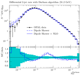
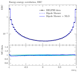
Separate fits have been performed for LO and NLO predictions. LO predictions have been obtained by running just the parton shower, using a one-loop running $\alpha_{s}$. NLO prediction have been obtained by means of supplementing the shower with the matrix element correction matching without using the Born screening cross section and a two-loop running $\alpha_{s}$. In total we find that the NLO simulation gives a marginally better fit than the LO one, though the description of data is completely comparable within experimental uncertainties.

Figure 3: Some event shape variables as predicted by the leading order and next-to-leading order simulations. Here, we additionally compare to the standard Herwig++ shower (version 2.5.1 with default settings), showing that the dipole shower gives a significantly improved description already at leading order.

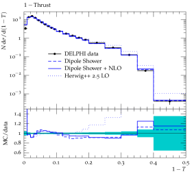
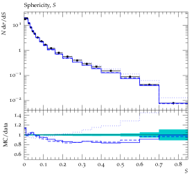
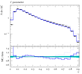
The fitted parameter values are displayed in Tab. 2. Most notably, the hadronization parameters for the LO and NLO fit do not significantly differ. For both predictions, a modification of the infrared running of $\alpha_{s}$ seems not to be preferred. The infrared cutoff of the parton shower is determined more precisely by the NLO fit, which prefers a smaller cutoff. Also $\alpha_{s}(M_{Z}^{2})$ is determined more precisely by the NLO fit. Both $\alpha_{s}$ values obtained are compatible with the world average PDG:2010 of $0.1184$, where the NLO result is closer to this value. Note that this should be regarded a coincidence at the level of the approximation considered and it is certainly not possible to uniquely relate the obtained value to one applying to the $\overline{MS}$ scheme. In Figs. 3 and 4 the LO and NLO simulation results are compared for selected observables. Fig. 5 shows the energy-energy-correlation, which has not been included in the fit.

Figure 4: The differential three jet rate as predicted by the leading order and next-to-leading order simulations.

Figure 5: Energy-energy correlation. Note that this observable has not been included in the fit.

4.1 Comparison of Matching Strategies

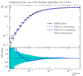
The Matchbox framework provides the facility to switch between the powheg-type matching with matrix element corrections including or excluding the auxiliary Born screening cross section, and subtractive matching. For reasons of systematics it is instructive to compare these approaches. No separate fit for the variants not considered so far has been performed and the NLO fit values as given in the previous section have been used. The different matching strategies give completely comparable results. If there are small visible differences, there is no clear tendency that either variant would give a better description than any of the others. Fig. 6 compares the matching strategies for the two jet rate. To this extent, the subtractive matching could be preferred amongst the powheg-type ones owing to its smaller computational complexity. This statement, however, not only includes that negative weighted events do not pose a major problem, but also has to be verified in a process dependent matter since there is no hint, if the behaviour observed here is a general feature – particularly at hadron colliders.

Figure 6: Comparison of matching strategies exemplified for the Durham two-jet rate.

5 Results at HERA

Owing to the approximation underlying the dipole parton shower, diagrams contributing to parton emission of a given dipole $(i,j)$ may be considered a gauge invariant subset in the soft and/or collinear limits for $N_{c}\to\infty$. This implies that the infrared cutoffs and soft scales entering the emission probabilities need not be the same for all dipoles. The emitter-spectator configurations forming gauge invariant quantities in this sense are the two emitter choices for final-final dipoles, initial-initial dipoles, and the combination of initial-final and final-initial configurations. Fitting DIS data therefore allows one to fix the infrared cutoff and soft scale for the latter, before finally constraining the same parameters for initial-initial dipoles at a hadron collider, which is considered in the next section.

For the fit described here, the same technique as for LEP, and data accumulated by the H1 experiment Adloff:1999ws have been used. For LO and NLO, the default Herwig++ PDFs, MSTW 2008 LO** Martin:2009iq ; Sherstnev:2007nd and MRST 2002 NLO Thorne:2002mr , have been used. The same PDFs were considered for hadron collider data to be discussed in the next section. The NLO fit was obtained by running the matching with matrix element correction.

The findings are similar as for the fit to LEP data. We find a reasonable prediction of transverse energy flows over the whole range of $(x,Q^{2})$ plane. The matched NLO prediction gives a comparable fit to the LO simulation, while preferring both a smaller infrared cutoff and screening scale. The fitted parameters are given in Tab. 3.

Figure 7: Average transverse energy in the central region as measured at HERA and compared to leading order and next-to-leading order predictions.

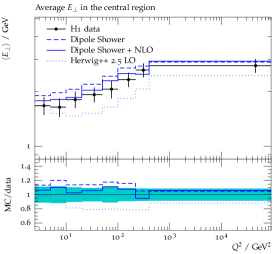
Fig. 7 shows the average transverse energy as a function of $Q^{2}$ in the central detector region. This observable is clearly improved by the NLO matching at small momentum transfers. A more detailed analysis of DIS data including inclusive jet and event shape data is currently underway.

6 Results at the Tevatron

After having determined the simulation parameters for hadronization, final state radiation, and radiation off a final-initial dipole by fitting LEP and HERA data, two parameters remain to be determined: the infrared cutoff and soft scale for radiation off an initial-initial dipole. We here consider the $p_{\perp}$ spectrum of $e^{+}e^{-}$ Drell-Yan pair production as measured by the CDF collaboration Affolder:1999jh . Since the Drell-Yan process receives rather large QCD corrections from leading to next-to-leading order and a still considerable correction at NNLO, both fits have been performed by normalising the simulation to the measured cross section. The matrix element matching including the Born screening cross section has been used here, as for the DIS data.

The Professor algorithm here turned out not to be applicable, as the cubic interpolation was not capable of describing the complete dynamics of letting the shower evolve to rather small infrared cutoffs, owing to the prescription of introducing a soft scale in $\alpha_{s}$ as already described before. We have therefore performed a preliminary fit by generating $300$ random points uniformly in parameter space, which here includes the infrared cutoff for initial-initial dipoles, the soft scale for initial-initial dipoles, as well as the widths of a Gaussian distribution for intrinsic transverse momentum, $\Lambda_{\perp}$. The latter has been chosen to be potentially different for valence and sea partons.

Out of these random points we have picked the one with lowest $\chi^{2}$ with respect to the data, again both for LO and NLO simulations. The resulting parameters are given in Tab. 4. Note that the $p_{\perp}$ distribution for sea partons is narrower, corresponding to a broader spatial distribution as can be motivated on different grounds.

Figure 8: Differential cross section of the Drell-Yan-pair $p_{\perp}$ compared to LO and NLO predictions. Note that the cross sections have been normalised to the measured one.

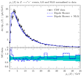
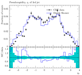
We show the comparison of LO and NLO simulations in Fig. 8 showing similar systematics to the distributions discussed before. In order to determine the predictivity of the simulation already at this very coarse level of tuning, we additionally show the pseudo-rapidity distribution of a third jet in events with at least two hard jets, Fig. 9, as carried out at CDF Abe:1994nj . Reasonable agreement with data is found. On top of the work presented in Platzer:2009jq , this constitutes another crucial test of coherent parton evolution.

Figure 9: The pseudo-rapidity distribution of a third jet in events with at least two jets. We here only show the leading order prediction in order to check the predictivity of the tune carried out so far.

7 Conclusions

We have introduced a new dipole shower module for the event generator Herwig++ that allows for an automatic matching of NLO computations with a parton shower. A tune of the hadronization module to the most important data sets show that we can achieve very good results from this simulation already without the inclusion of NLO terms. Including NLO corrections at this relatively simple level only marginally improves the results. This effect is expected as it is known that the Catani–Seymour showers tend to mimic the behaviour of NLO matrix elements very well also in phase space regions well outside the collinear limits. However, the matching poses no technical problem and can be seen as a proof–of–concept for the idea to provide a framework for automatic matching. At this time with relatively simple matrix elements at NLO that are provided by internal code. Future work will concentrate in the inclusion of external code via a well defined interface, following the ideas in Binoth:2010xt .

Appendix A Code Validation

A.1 Shower Splitting Kernels

The sampling of shower splitting kernels has been explicitly verified in situ, meaning using the full implementation as present in the simulation code, against an independent implementation using a numerical integration to obtain the Sudakov-type distributions. Fig. 10 shows an example for a final-final splitting kernel, proving correctness of this part of the code.

Figure 10: Example comparison of sampled final-final splitting momentum fraction (blue lines) versus results from a numerical integration (turquoise lines) at two different dipole masses, $s_{ij}=(100{\rm GeV})^{2}$ (continuous lines) and $s_{ij}=(50{\rm GeV})^{2}$ (broken lines).

A.2 NLO QCD Corrections

All leading order matrix elements implemented in the Matchbox framework have been cross-checked against the Herwig++ matrix elements.

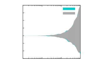
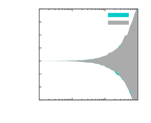
The functionality of the automatically generated subtraction terms has been verified. Fig. 11 shows a typical examples of the ratio of subtraction to real emission cross section, plotted against each of the invariants entering the propagator denominators.

Figure 11: Envelopes of the ratio of the subtraction to the real emission cross section versus the propagator denominator for all singular configurations in $Z+{\rm jet}$ production.

The ‘plain’ NLO cross section, and the inclusive one entering the matching with matrix element correction have been checked to agree, with and without the usage of the Born ‘screening’ cross section. The NLO cross section for $e^{+}e^{-}\to{\rm jets}$ has been validated against the analytically known $K$-factor of $1+\alpha_{s}/\pi$. The NLO cross section for DIS and Drell-Yan has been checked against the existing powheg implementation in Herwig++. For deep inelastic scattering, the subtraction terms have been modified in order to have positive definite dipole kernels, finite terms of the integrated subtraction terms have been changed accordingly. The functionality of the subtraction has been checked with both variants, and the NLO cross sections with and without modifications are found to agree.

A.3 NLO Matching with Matrix Element Corrections

A non-trivial cross check of the matrix element correction code and ExSample as the underlying ‘working horse’, is to consider the spectra for a gluon emission off a $q\bar{q}$ dipole as generated by the shower, which is validated against a numerical integration of the expected distribution implemented in a completely independent code. By putting the real emission matrix element entering the matching to be equal to the sum of dipoles (the correctness of which has been checked by verifying that the cross section of the subtracted real emission matrix element is consistent with zero), the matrix element correction must produce the same spectrum as the shower code. We have checked that this is indeed the case. It should be stressed that the machinery underlying the setup of the matrix element correction is much more complex than the shower implementation, and, that the splitting kernel entering the matrix element correction does depend on more parameters than the one parameter of the shower kernel (corresponding to the dipole invariant mass).

Parameter	Range	Description
$\alpha_{s}(M_{Z}^{2})$	$0.1-0.13$	Input $\alpha_{s}$ at $Z$ mass.
$\mu_{IR,FF}$	$0.5\ {\rm GeV}-2.0\ {\rm GeV}$	Infrared cutoff for final-final dipoles
$\mu_{\text{soft},FF}$	$0.0\ {\rm GeV}-1.2\ {\rm GeV}$	Soft scale for final-final dipoles
$m_{g,c}$	$0.67\ {\rm GeV}-3.0\ {\rm GeV}$	Gluon constituent mass
$\text{Cl}_{\text{max}}$	$0.5\ {\rm GeV}-10\ {\rm GeV}$	Maximum cluster mass
$\text{Cl}_{\text{pow}}$	$0.0-10.0$	Cluster mass exponent
$\text{Cl}_{\text{smr}}$	$0.0-10.0$	Cluster direction smearing
$P_{\text{split}}$	$0.0-1.4$	Cluster mass splitting parameter

Table 1: The parameters varied for the fit to LEP data.

Parameter	LO	NLO
$\alpha_{s}(M_{Z}^{2})$	$0.113185\pm 0.007281$	$0.117550\pm 0.005053$
$\mu_{IR,FF}$	$(1.416023\pm 0.306430)\ {\rm GeV}$	$(1.245196\pm 0.226821)\ {\rm GeV}$
$\mu_{\text{soft},FF}$	$(0.242725\pm 0.202069)\ {\rm GeV}$	$0.0\ {\rm GeV}$
$m_{g,c}$	$(1.080386\pm 0.499546)\ {\rm GeV}$	$(1.007680\pm 0.265565)\ {\rm GeV}$
$\text{Cl}_{\text{max}}$	$(4.170320\pm 0.589504)\ {\rm GeV}$	$(3.664004\pm 0.639504)\ {\rm GeV}$
$\text{Cl}_{\text{pow}}$	$5.734681\pm 1.006965$	$5.687022\pm 0.869322$
$\text{Cl}_{\text{smr}}$	$4.548755\pm 2.350193$	$3.115744\pm 2.436793$
$P_{\text{split}}$	$0.765173\pm 0.074008$	$0.771329\pm 0.074248$

Table 2: Parameters for LO and NLO fits to LEP data.

Parameter	LO	NLO
$\mu_{IR,FI}$	$(0.796205\pm 0.333340)\ {\rm GeV}$	$(0.718418\pm 0.210448)\ {\rm GeV}$
$\mu_{\text{soft},FI}$	$(1.355894\pm 0.432515)\ {\rm GeV}$	$(1.003714\pm 0.252398){\rm GeV}$

Table 3: Parameters for LO and NLO fits to HERA data.

Parameter	LO	NLO
$\mu_{IR,II}$	$0.367359\ {\rm GeV}$	$0.275894\ {\rm GeV}$
$\mu_{\text{soft},II}$	$0.205854\ {\rm GeV}$	$0.254028\ {\rm GeV}$
$\Lambda_{\perp,\text{valence}}$	$1.68463\ {\rm GeV}$	$1.26905\ {\rm GeV}$
$\Lambda_{\perp,\text{sea}}$	$1.29001\ {\rm GeV}$	$1.1613\ {\rm GeV}$

Table 4: Parameters for LO and NLO fits to the CDF Drell-Yan data.

References

- (1) M. Bähr et al., Eur. Phys. J. C58, 639 (2008), 0803.0883.
- (2) G. Corcella et al., (2002), hep-ph/0210213.
- (3) T. Sjöstrand, S. Mrenna, and P. Skands, Comput. Phys. Commun. 178, 852 (2008), 0710.3820.
- (4) T. Sjöstrand, S. Mrenna, and P. Skands, JHEP 05, 026 (2006), hep-ph/0603175.
- (5) T. Gleisberg et al., JHEP 02, 007 (2009), 0811.4622.
- (6) M. H. Seymour, Comp. Phys. Commun. 90, 95 (1995), hep-ph/9410414.
- (7) E. Norrbin and T. Sjöstrand, Nucl. Phys. B603, 297 (2001), hep-ph/0010012.
- (8) S. Catani, F. Krauss, R. Kuhn, and B. R. Webber, JHEP 11, 063 (2001), hep-ph/0109231.
- (9) L. Lönnblad, JHEP 05, 046 (2002), hep-ph/0112284.
- (10) F. Krauss, JHEP 08, 015 (2002), hep-ph/0205283.
- (11) S. Hoeche et al., (2006), hep-ph/0602031.
- (12) N. Lavesson and L. Lönnblad, JHEP 04, 085 (2008), 0712.2966.
- (13) S. Hoeche, F. Krauss, S. Schumann, and F. Siegert, JHEP 05, 053 (2009), 0903.1219.
- (14) K. Hamilton, P. Richardson, and J. Tully, (2009), 0905.3072.
- (15) B. Pötter, Phys. Rev. D63, 114017 (2001), hep-ph/0007172.
- (16) B. Pötter and T. Schörner, Phys. Lett. B517, 86 (2001), hep-ph/0104261.
- (17) M. Dobbs, Phys. Rev. D65, 094011 (2002), hep-ph/0111234.
- (18) S. Frixione and B. R. Webber, JHEP 06, 029 (2002), hep-ph/0204244.
- (19) S. Frixione, P. Nason, and B. R. Webber, JHEP 08, 007 (2003), hep-ph/0305252.
- (20) S. Frixione, E. Laenen, P. Motylinski, and B. R. Webber, JHEP 03, 092 (2006), hep-ph/0512250.
- (21) S. Frixione, E. Laenen, P. Motylinski, and B. R. Webber, JHEP 04, 081 (2007), hep-ph/0702198.
- (22) S. Frixione, E. Laenen, P. Motylinski, B. R. Webber, and C. D. White, JHEP 07, 029 (2008), 0805.3067.
- (23) S. Frixione, F. Stoeckli, P. Torrielli, and B. R. Webber, JHEP 1101, 053 (2011), 1010.0568.
- (24) P. Nason, JHEP 11, 040 (2004), hep-ph/0409146.
- (25) S. Frixione, P. Nason, and G. Ridolfi, (2007), 0707.3081.
- (26) P. Nason and G. Ridolfi, JHEP 08, 077 (2006), hep-ph/0606275.
- (27) S. Frixione, P. Nason, and G. Ridolfi, JHEP 09, 126 (2007), 0707.3088.
- (28) S. Alioli, P. Nason, C. Oleari, and E. Re, JHEP 07, 060 (2008), 0805.4802.
- (29) S. Alioli, P. Nason, C. Oleari, and E. Re, JHEP 04, 002 (2009), 0812.0578.
- (30) S. Alioli, K. Hamilton, P. Nason, C. Oleari, and E. Re, JHEP 1104, 081 (2011), 1012.3380.
- (31) K. Hamilton, P. Richardson, and J. Tully, JHEP 10, 015 (2008), 0806.0290.
- (32) K. Hamilton, P. Richardson, and J. Tully, JHEP 04, 116 (2009), 0903.4345.
- (33) K. Hamilton, JHEP 1101, 009 (2011), 1009.5391.
- (34) L. D’Errico and P. Richardson, (2011), 1106.2983.
- (35) L. D’Errico and P. Richardson, (2011), 1106.3939.
- (36) S. Hoche, F. Krauss, M. Schonherr, and F. Siegert, JHEP 1104, 024 (2011), 1008.5399.
- (37) S. Gieseke, P. Stephens and B.R. Webber, JHEP 12, 045 (2003), hep-ph/0310083.
- (38) T. Sjöstrand and P. Z. Skands, Eur. Phys. J. C39, 129 (2005), hep-ph/0408302.
- (39) S. Catani and M.H. Seymour, Nucl. Phys. B485, 291 (1997), hep-ph/9605323.
- (40) S. Catani, S. Dittmaier, M. H. Seymour, and Z. Trocsanyi, Nucl. Phys. B627, 189 (2002), hep-ph/0201036.
- (41) S. Schumann and F. Krauss, JHEP 03, 038 (2008), 0709.1027.
- (42) M. Dinsdale, M. Ternick and S. Weinzierl, Phys. Rev. D76, 094003 (2007), 0709.1026.
- (43) Z. Nagy and D. E. Soper, JHEP 10, 024 (2005), hep-ph/0503053.
- (44) W. T. Giele, D. A. Kosower, and P. Z. Skands, Phys. Rev. D78, 014026 (2008), 0707.3652.
- (45) O. Latunde-Dada, S. Gieseke, and B. Webber, JHEP 02, 051 (2007), hep-ph/0612281.
- (46) A. van Hameren, C. Papadopoulos, and R. Pittau, JHEP 0909, 106 (2009), 0903.4665.
- (47) V. Hirschi et al., JHEP 1105, 044 (2011), 1103.0621.
- (48) G. Ossola, C. G. Papadopoulos, and R. Pittau, JHEP 0803, 042 (2008), 0711.3596.
- (49) C. Berger et al., Phys.Rev.Lett. 102, 222001 (2009), 0902.2760.
- (50) C. Berger et al., Phys.Rev.Lett. 106, 092001 (2011), 1009.2338.
- (51) W. Giele and G. Zanderighi, JHEP 0806, 038 (2008), 0805.2152.
- (52) P. Mastrolia, G. Ossola, T. Reiter, and F. Tramontano, JHEP 1008, 080 (2010), 1006.0710.
- (53) G. Heinrich, G. Ossola, T. Reiter, and F. Tramontano, JHEP 1010, 105 (2010), 1008.2441.
- (54) T. Gleisberg and F. Krauss, Eur.Phys.J. C53, 501 (2008), 0709.2881.
- (55) K. Hasegawa, S. Moch, and P. Uwer, Comput.Phys.Commun. 181, 1802 (2010), 0911.4371.
- (56) R. Frederix, T. Gehrmann, and N. Greiner, JHEP 1006, 086 (2010), 1004.2905.
- (57) R. Frederix, S. Frixione, F. Maltoni, and T. Stelzer, JHEP 10, 003 (2009), 0908.4272.
- (58) K. Hamilton and P. Nason, JHEP 1006, 039 (2010), 1004.1764.
- (59) S. Hoche, F. Krauss, M. Schonherr, and F. Siegert, (2010), 1009.1127.
- (60) S. Platzer and S. Gieseke, JHEP 1101, 024 (2011), 0909.5593.
- (61) B. R. Webber, Nucl. Phys. B238, 492 (1984).
- (62) S. Platzer, (2011), 1108.6182.
- (63) DELPHI, P. Abreu et al., Z. Phys. C73, 11 (1996).
- (64) JADE, P. Pfeifenschneider et al., Eur. Phys. J. C17, 19 (2000), hep-ex/0001055.
- (65) A. Buckley et al., (2010), 1003.0694.
- (66) A. Buckley, H. Hoeth, H. Lacker, H. Schulz, and J. E. von Seggern, Eur. Phys. J. C65, 331 (2010), 0907.2973.
- (67) S. Gieseke, M. H. Seymour, and A. Siodmok, JHEP 06, 001 (2008), 0712.1199.
- (68) Particle Data Group, K. Nakamura et al., J. Phys. G 37, 075021 (2010).
- (69) H1, C. Adloff et al., Eur. Phys. J. C12, 595 (2000), hep-ex/9907027.
- (70) A. D. Martin, W. J. Stirling, R. S. Thorne, and G. Watt, Eur. Phys. J. C63, 189 (2009), 0901.0002.
- (71) A. Sherstnev and R. S. Thorne, Eur. Phys. J. C55, 553 (2008), 0711.2473.
- (72) R. S. Thorne, A. D. Martin, W. J. Stirling, and R. G. Roberts, Acta Phys. Polon. B33, 2927 (2002), hep-ph/0207067.
- (73) CDF, A. A. Affolder et al., Phys. Rev. Lett. 84, 845 (2000), hep-ex/0001021.
- (74) CDF Collaboration, F. Abe et al., Phys.Rev. D50, 5562 (1994).
- (75) T. Binoth et al., Comput.Phys.Commun. 181, 1612 (2010), 1001.1307, Dedicated to the memory of, and in tribute to, Thomas Binoth, who led the effort to develop this proposal for Les Houches 2009.