The 2d Gross-Neveu Model for Pseudovector Fermions and Tachyonic Mass Generation

Abstract

Recent observations in the OPERA experiment suggest that the neutrino could propagate with speed that is superluminal. Based on early theoretical work on tachyonic fermions we shall study a modification of the Gross-Neveu model in two dimensions. We shall see that the theory results to the dynamical generation of real and imaginary masses. These imaginary masses indicate the possibility that tachyonic solutions (or instabilities) could exist in the theory. The implications of a tachyonic neutrino coming from astrophysical sources are critically discussed. Moreover, we present a toy model that consists of an $U(2,2)$ invariant Dirac Lagrangian. This theory can have tachyonic masses as solutions. A natural mass splitting between the solutions is a natural outcome of the formalism.

Modified 2d Gross-Neveu Model and Extrema of the Effective Potential

The Gross-Neveu model describes Dirac fermions in 1+1 dimensions, that have four fermions interactions, thus being a very elegant and useful tool for studies of the strong interactions. It is based on non-perturbative techniques, namely the large N expansion and it results to the dynamical generation of a fermionic mass, a phenomenon known as dimensional transmutation. It is described by the Lagrangian density

$$\mathcal{L}=\sum_{i}^{N}i\bar{\psi}_{i}\gamma^{\mu}\partial_{\mu}\psi_{i}+\frac{1}{2}g_{0}^{2}\Big{(}\sum_{i}^{N}\bar{\psi}_{i}\psi_{i}\Big{)}^{2}$$ (1)

for $i=1,2,...N$. The Lagrangian (1) is invariant under the chiral symmetry $\psi_{i}\rightarrow\gamma_{5}\psi_{i}$. This symmetry is a kind of $Z_{2}$ symmetry, since $\gamma_{5}^{2}=1$. Due to one-loop quantum corrections, this symmetry is broken by the theory.

Recently an experimental result has put into question the nature of the neutrino. Particularly, the OPERA experiment [1] resulted that the neutrino propagates in space with speed that exceeds the speed of light. It is obvious that the experimental results must be re-examined in order to be sure that this result is valid. Nevertheless it is an intriguing result that deserves some attention and if proven true, much of the theoretical work involving the neutrino must be put in a new conceptual basis. Actually it has draw the attention of many theorists [2, 3, 4, 5, 6, 7, 8, 9, 10, 11, 12, 13, 14, 15, 16].

Insightful studies on the tachyonic nature of the neutrino was provided in the 80’s by A. Chodos et. al [18, 19, 20]. The authors proposed experiments that could prove the tachyonic nature of the neutrino field. They actually proposed the time of flight experiment, which is an OPERA-like experiment. Up to now, several papers followed, studying the tachyonic neutrino [21, 22, 23, 24, 25, 26, 27, 28, 29, 30]. The Lagrangian that describes the tachyonic neutrino is given by [18]:

$$\mathcal{L^{\prime}}=i\bar{\psi}\gamma_{5}\gamma^{\mu}\partial_{\mu}\psi-m\bar{\psi}\psi$$ (2)

In the massless case, at the Standard Model level, the terms $i\bar{\psi}\gamma_{5}\gamma^{\mu}\partial_{\mu}\psi$ and $i\bar{\psi}\gamma^{\mu}\partial_{\mu}\psi$, are indistinguishable.

In this brief letter we shall modify the Gross-Neveu Lagrangian according to the massless limit of the tachyonic Lagrangian (2). The modified Gross-Neveu Lagrangian is:

$$\mathcal{L}=\sum_{i}^{N}i\bar{\psi}_{i}\gamma_{5}\gamma^{\mu}\partial_{\mu}\psi_{i}+\frac{1}{2}g_{0}^{2}\Big{(}\sum_{i}^{N}\bar{\psi}_{i}\psi_{i}\Big{)}^{2}$$ (3)

We shall dwell on the mass generation issues, and how the results are modified when using the above Lagrangian. We must note that the massless field theory of the tachyons does not suffer from the conceptual problems that the massive case has. Indeed no consistent Quantum field theory of tachyons exists up to now [18], however it could be a good starting point to work towards the consistent incorporation of tachyons in the successful field theories. The Lagrangian (3) is invariant under the chiral transformation $\psi_{i}\rightarrow\gamma_{5}\psi_{i}$. We now compute the effective potential corresponding to (3). Using very well known techniques [31] we have:

$$\int\mathcal{D}\psi\mathcal{D}\bar{\psi}e^{-i\int\mathrm{d}x^{D}V_{eff}(\sigma)}=\int\mathcal{D}\psi\mathcal{D}\bar{\psi}\exp\Big{[}\int\mathrm{d}x^{D}\Big{(}i\bar{\psi}_{i}\gamma_{5}\gamma^{\mu}\partial_{\mu}\psi_{i}-\frac{1}{2}g_{0}^{2}\sigma^{2}-\mu\sigma\bar{\psi}_{i}\psi_{i}\Big{)}\Big{]}$$ (4)

where $\sigma$ is a composite field in terms of which we shall express the final expression of the effective potential. In the above, $\mu$ is a free parameter to be used for dimensional reasons and $D=2-2\epsilon$. After performing the Gaussian integration over the fermions and taking the $\epsilon\rightarrow 0$ we obtain:

$$e^{-i\int\mathrm{d}x^{D}V_{eff}(\sigma)}=\exp\Big{[}i\int\mathrm{d}x^{D}\Big{(}-\frac{1}{2g^{2}}\sigma^{2}+\frac{N}{4\pi}(\frac{1}{\epsilon}-\gamma+\ln(4\pi))\sigma^{4}-\frac{N}{4\pi}\sigma^{4}\ln\frac{\sigma^{4}}{\mu^{4}}\Big{)}\Big{]}$$ (5)

Using the $\mathrm{\overline{MS}}$ renormalization scheme to subtract the poles, the effective potential reads:

$$V_{eff}(\sigma)=\frac{1}{2g^{2}}\sigma^{2}+\frac{N}{4\pi}\sigma^{4}\Big{(}\ln\frac{\sigma^{4}}{\mu^{4}}-1\Big{)}$$ (6)

Minimizing the effective potential in respect to the parameter $\sigma$, we obtain the equation:

$$\frac{1}{2g^{2}}+\frac{N}{2\pi}\sigma^{2}\ln(\frac{\sigma^{4}}{\mu^{4}})=0$$ (7)

The above equation can have four real roots of the form $(x_{1},-x_{1})$ and ($x_{2},-x_{2}$), with $x_{1},x_{2}$ real positive number. This result is similar to the usual Gross-Neveu result. This means that $\sigma$ can take four real values, $\sigma=\pm x_{1}$ and $\sigma=\pm x_{2}$. The field $\sigma$ is the minimum of the effective potential, thus the quantum theory can have two equivalent ground states.

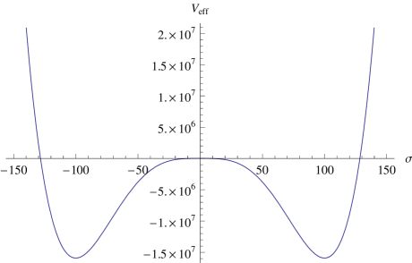
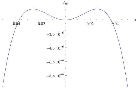
Figure 1: The effective potential for $g^{2}N/\mu\sim 10$. In the left figure we can see the minima of the potential at $\sigma_{1}=100$ and $\sigma_{2}=-100$. In the right figure we can see the maxima of the potential $\sigma_{3}=0.0091$, $\sigma_{4}=-0.0091$

The fermions acquire finite masses which can be $m=|\sigma|=x_{1}$ and $m=|\sigma|=x_{2}$. It is obvious that the initial $Z_{2}$ chiral symmetry is broken. Additionally, the fermionic fields can have two different values for their mass, which is dynamically generated. The modified Gross-Neveu model we studied results to two equal masses (minima of the potential), a result similar to the original Gross-Neveu result. But the most intriguing difference in comparison to the Gross-Neveu is the existence of complex extremal points of the effective potential. Indeed a numerical study of the above equation (7) shows that there are values of the expression $\frac{\pi\mu}{g^{2}N}$ for which the equation has two complex roots. These roots indicate instability of the quantum theory, since the mass-square of the field $\sigma$ can be negative. But in view of the new experimental data we could argue that the above model (3) can generate dynamically tachyonic masses. Recalling that the modified version of the Gross-Neveu we studied is based on a tachyonic Lagrangian, the fact that solutions for tachyonic masses exist, can be very useful.

Let us give here some quantitative details of the calculation we performed. Recall that the original two dimensional Gross-Neveu model was described by the effective potential $V^{\prime}_{eff}$,

$$V^{\prime}_{eff}=\frac{1}{2g^{2}}\sigma^{2}+\frac{N}{4\pi}\sigma^{2}\Big{(}\ln\frac{\sigma^{2}}{\mu^{2}}-1\Big{)}$$ (8)

The minimization process results to the following equation:

$$\frac{1}{2g^{2}}+\frac{N}{4\pi}\ln\frac{\sigma^{2}}{\mu^{2}}=0$$ (9)

It is obvious that equation (9) has only two real roots. In addition, if one tries to search for roots of the form $\sigma=ix$, this results to mathematical inconsistencies. Hence no imaginary roots exists for the original two dimensional Gross-Neveu model. In the case of (7), we have a plethora of roots. The most interesting are these of the form $\sigma=ix$. Indeed, one can easily check numerically that if we put $\sigma=ix$, then we wave two real solutions for $x$, namely $x$ and $-x$. Hence the result is that, equation (7) has two purely imaginary roots, $\sigma=ix$ and $\sigma=-ix$ For example, if $Ng^{2}=10^{12}$ (large N-strong coupling limit) and $\mu=10^{6}$, then $\sigma_{1}=10^{-7}i$ and $\sigma_{2}=-10^{-7}i$. Therefore we have two equivalent tachyonic mass vacuum state solutions. Apart from purely imaginary solutions, equation (7) has complex roots of the form $\sigma=a+bi$, and as we mentioned earlier real roots. Let us discuss the implications of the complex roots at this point. Complex masses are very closely related to tachyonic fermion solutions. Indeed, a generalized form of Lagrangian (3), found in [29], results in the modified Dirac equation [29]:

$$(i\gamma^{\mu}\partial_{\mu}-\lambda_{T})\psi=0$$ (10)

with $\lambda_{T}=ia+b\gamma_{5}$. Under certain conditions, depending on the $a$ and $b$ choices, one can obtain tachyonic solutions in this case, but there are two more solutions. The authors of [29] call these ”luxons” and ”bradyons”. To us, these solutions are under serious investigation, since the solutions lead to serious quantization problems, more severe than the tachyonic solutions. In any case, if superluminal propagation in spacetime is true, then we should work and find a consistent quantization procedure, even by generalizing the theoretical formalism of quantization. As for the real roots that equation (7) has, the first set $\pm x_{1}$ are local maxima and the other set $\pm x_{2}$ are local minima. Hence the situation is equivalent to the 2d Gross-Neveu model, except the two maximum solutions. In figures 1 (a) (left) and (b) (right) we plot the effective potential (6), for $g^{2}N/\mu\sim 10$. We can clearly see the two minima, $\sigma_{1}=100$, $\sigma_{2}=-100$ and the two maxima $\sigma_{3}=0.0091$, $\sigma_{4}=-0.0091$. In figure 2 we have made a plot of the roots corresponding to equation (7), for various values of $g^{2}N/\mu$. The y-axis represents the imaginary axis, while the x-axis, the real axis. As we can see there are purely imaginary, complex and real roots.

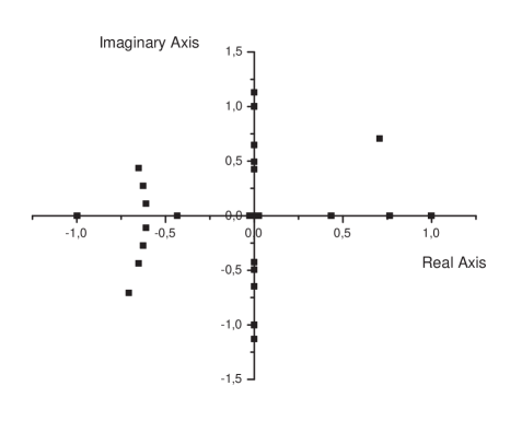
Figure 2: The minima of the effective potential $V_{eff}$ for various values of the parameters $g$, $\mu$ in the large $N$ limit

Before closing this investigation, let us study the effective potential in various limiting cases of the parameters. We start with the case $\frac{\sigma^{4}}{\mu^{4}}\ll 1$. Upon using the approximation for the logarithm, valid for $x>0$:

$$\ln x=2\sum_{k=1}^{\infty}\frac{1}{(2k-1)}\Big{(}\frac{x-1}{x+1}\Big{)}^{2k-1}$$ (11)

and keeping the first term in the sum, the effective potential $V_{eff}$ of equation (6) can be cast as:

$$V_{eff}(\sigma)=\frac{1}{2g^{2}}\sigma^{2}+\frac{N}{4\pi}\sigma^{4}\Big{(}\frac{\sigma^{4}}{\mu^{4}}-1\Big{)}$$ (12)

If we minimize equation (12) in respect to $\sigma^{2}$, we obtain the following solutions:

$$\sigma_{1}=\frac{1}{30}\Big{(}m+\frac{g^{2}Nm^{2}}{A}+\frac{A}{g^{2}N}\Big{)},$$ (13)

$$\sigma_{2}=\frac{1}{60}\Big{(}2m+\frac{\big{(}-1-i\sqrt{3}\big{)}g^{2}Nm^{2}}{A}+\frac{i\big{(}i+\sqrt{3}\big{)}A}{g^{2}N}\Big{)},$$

$$\sigma_{3}=\frac{1}{60}\Big{(}2m+\frac{i\big{(}i+\sqrt{3}\big{)}g^{2}Nm^{2}}{A}+\frac{\big{(}-1-i\sqrt{3}\big{)}A}{g^{2}N}\Big{)}$$

where we introduced the parameter $A$, which is equal to:

$$A=\sqrt[3]{m^{3}N^{3}g^{6}-2700mN^{2}\pi g^{4}+30\sqrt{6\pi}\sqrt{g^{8}m^{2}N^{4}\Big{(}1350\pi-g^{2}m^{2}N\Big{)}}}$$ (14)

In the case we have $\frac{\sigma^{4}}{\mu^{4}}\gg 1$, we cannot have analytic solutions. Nevertheless by using the approximation,

$$\ln x=-\mathrm{K}_{0}(x)-\gamma+\ln 2$$ (15)

and in addition, the asymptotic form of the modified Bessel function $\mathrm{K}_{0}(x)$, valid for large values of $x$:

$$\mathrm{K}_{0}(x)\sim\sqrt{\frac{\pi}{2x}}e^{-x}$$ (16)

we obtain a simpler expression for the effective potential. Indeed the potential can be written as:

$$V_{eff}(\sigma)=\frac{1}{2g^{2}}\sigma^{2}+\frac{N}{4\pi}\sigma^{2}\Big{(}\mu^{2}\sqrt{\frac{\pi}{2}}e^{-\frac{\sigma^{4}}{\mu^{4}}}-\gamma+\ln 2-2\Big{)}$$ (17)

The original Gross-Neveu model was renormalization scale invariant. We must say that the effective potential of the modified Gross-Neveu is also $\mu$-independent, as can be easily seen from the following equation

$$\mu^{2}\frac{\partial V_{eff}(\sigma)}{\partial\mu^{2}}=0$$ (18)

We shall not pursuit further the renormalization group issues in this paper.

A Discussion on Tachyonic Fermions and Their Impact on Physical Phenomena

In this section we discuss some issues in reference to the possible tachyonic nature of the neutrino. Obviously, the experimental results must be further scrutinized in order to be sure for their validity. However if true, the tachyonic nature of the neutrino could alter some aspects of physical processes or even give answers to unexplained mysteries. For example in hot-dense backgrounds, the plasmon decay and the effective neutrino-photon coupling must be reexamined in view of the tachyonic nature of the neutrino. The modification of the effective photon-neutrino interactions at high temperature could modify the neutrino emission from stars, or the neutrino emission from Gamma Ray Bursts. On that account, an interesting impact of superluminal neutrino’s is studied in [2]. In regards to Gamma Ray bursts, phenomenological results of quantum gravity predict that neutrino’s could arrive faster than the photons [32]. This result is quite interesting since the nature of the neutrino is controversial, and signals a strong relation of this particle with gravity, in an undiscovered way. In the 50’s Wheeler [33] had noted that the neutrino could be a geometrodynamical particle of some kind (in the next section we shall present an Poincare invariance violating extension of the Dirac equation, with interesting features nonetheless).

One outcome of the possible “tachyonicity” of the neutrinos is that, in order to be consistent, “tachyonicity” requires the existence of both right handed and left handed neutrinos. This is a problem for the neutrino since we have observed only left handed neutrinos. Nevertheless, this is already a problem of contemporary neutrino physics, which is solved by the seesaw mechanism [34].

A negative mass square can be a very strange physical result. However we must note that, the mass parameter even in classical mechanics, is a parameter that cannot be measured directly even for slow particles [35]. Only energy and momentum are measured through interactions and therefore must be real [35]. As noted by the authors of [35], the imaginary mass offends traditional thinking and not observable physics. Nonetheless, imaginary mass particles cannot be consistently quantized in the “traditional” quantum field theory way, as gravity cannot be quantized too. Perhaps this is another hint that makes us speculate about the possible interconnection of gravity and the neutrino field.

Another quite astonishing feature of tachyonic fermions is that, if such a particle loses energy in a medium, it will undergo an acceleration [35]. If we assume that the neutrino is a tachyon, there is no direct way for this particle to loose energy, due to the fact that it has no electric charge. Nevertheless, it is known that a neutrino travelling through a medium can have leading order matter induced magnetic and electric dipole moments [36]. The last can be non-zero even for Majorana neutrinos. It is not likely to directly measure such effects, however if the neutrino is proven to be tachyon, then these interactions could make the neutrino loose energy in various dense medium. This could have observable effects coming from astrophysical sources and astrophysical events. Since the energy loss of a tachyon causes it’s acceleration, then neutrinos loosing energy in a Gamma Ray Burst generating background, would eventually accelerate and would reach earth faster than a photon. This result is similar to the quantum gravity one, we discussed earlier.

Relativistic Quantum Mechanics, Localization and A-causality and Superluminal Propagation

In this section we shall discuss a curious and rather not so very well known problem that appears in the relativistic Dirac equation. We base our analysis in [37]. It is known that any solutions of the Dirac equation cannot describe propagation faster than light. However in the Foldy-Wouthuysen representation (a unitary transformation of the Dirac and other operators, that transforms the Dirac equation into two Klein-Gordon equations), superluminal propagation is possible, in terms of a superluminal spreading of the wave functions. This problem is very closely related to position operators commuting with the positive energy and in addition to the way we define localization of a particle. If we assume a quantum mechanical-consistent definition of the localization of a particle in a subspace $B$ of $R^{3}$, then there is a non-zero probability that this particle can be found outside this space $B$, at a space $B_{0}$. This instantaneous spreading of the wave functions corresponds to superluminal propagation. The whole argument can be summarized in terms of the following theorem, which states that:

Let $D$ be a Hilbert space. For every set $B\subset R^{3}$ let $F(B)$ be a bounded self adjoint operator in $D$, such that for every function $\psi$ belonging in $D$ with $\langle\psi|\psi\rangle=1$, the probability measure $\langle\psi|F(B)|\psi\rangle$ satisfies the following properties:

• $\langle\psi|F(B)|\psi\rangle=1$ and $\langle\phi|F(B)|\phi\rangle=0$ implies $\langle\phi|\psi\rangle=1$

• There is a self adjoint operator $p$ (the generator of space translations) such that for all $a$ $\epsilon$ $R^{3}$,

  $\langle e^{-ipa}\psi|F(B+a)|e^{-ipa}\psi\rangle=\langle\psi|F(B)|\psi\rangle$

Furthermore define a non-constant positive operator $H(p)$. For all non empty sets $B_{i}\subset R^{3}$ and for all $\varepsilon>0$, there exists a time $t$ $\epsilon$ (0,$\varepsilon$), for which

$$\langle e^{-iHt}\psi|F(B_{i})|e^{-iHt}\psi\rangle\neq 0$$ (19)

Therefore if $F(B_{i})$ represents a position operator, there is a small probability that the particle can be outside $B_{i}$, to another subset of $R^{3}$ for arbitrarily small time. It is expected that in physically reasonable situations, this instantaneous spreading of the wave functions must be very small. For a much more detailed analysis we refer the reader to reference [37] (page 30).

An $U(2,2)$-invariant Modification of the Dirac Equation

The standard Dirac Lagrangian in curved spacetime is built as a gauge theory on a manifold $M$, with $SL(2,C)$ structural group. The vielbeins $e_{\mu}^{A}$ are the sections of the corresponding principal bundle, the spin connections $\omega^{r}_{s\mu}$ are corrections of the principal bundle, and the fields $\psi_{r}$ are the sections of the associate bundle with fibre $C^{4}$. A more general spinor equation in curved space can be built if we admit the structural group to be the total pseudo-unitary group $U(2,2)$, to which $SL(2,C)$ is an injected subgroup [38]. The group $U(2,2)$, is used in twistor geometry and conformal field theory. We shall consider a very simple form of the modified $U(2,2)$-Dirac Lagrangian (see [38] for details), by taking $e^{\mu}_{A}=\delta^{\mu}_{A}$, the internal metric to be locally Euclidean, that is $g_{\mu,\nu}=\delta_{\mu,\nu}$. The Lagrangian reads,

$$\mathcal{L}=V\frac{i}{2}\big{(}\bar{\psi}\gamma^{\mu}\partial_{\mu}\psi-\partial_{\mu}\bar{\psi}\gamma^{\mu}\psi\big{)}-W\bar{\psi}\psi+U\partial^{\mu}\bar{\psi}\partial_{\mu}\psi$$ (20)

The corresponding equation of motion is,

$$Vi\gamma^{\mu}\partial_{\mu}\psi-W\psi-U\partial^{\mu}\partial_{\mu}\psi=0$$ (21)

with $V,W,U$, real constants (some of these have mass dimensions). The above equation does not correspond to any relativistic equation of an elementary particle, since no representation of the Poincare group results in equation (21). In addition, the quantization of the above equation is not usual in the traditional Quantum Field Theory-way because tachyonic solutions appear, and obviously due to the second derivatives in (21). Nevertheless we think that (21) describes a particle dynamical system not respecting Poincare invariance in 4-dimensions. The reason for considering such an physics-unattractive equation, is due to the outcomes, in reference to tachyonic solutions. Indeed, if the solutions of (21) are of the form, $\psi=\phi e^{-ip_{\mu}x^{\mu}}$, then equation (21), becomes:

$$\gamma^{\mu}p_{\mu}\phi=m\phi$$ (22)

with two solutions for the mass, namely:

$$m_{1,2}=\Big{(}\frac{1}{2U^{2}}\big{(}2UW+V^{2}\pm\sqrt{V^{4}+4UWV^{2}}\big{)}\Big{)}^{1/2}$$ (23)

Therefore, the solutions to (21), correspond to a superposition of two Dirac waves with masses $m_{1},m_{2}$. There are values in the parameter space for which the masses can be purely imaginary. This means that we may have tachyonic solutions for the wave particle $\psi$. In addition there is a mass gap between the two masses. This means that if we choose appropriately the parameters, we can obtain a large mass gap between the masses $m_{1}$ and $m_{2}$. If we consider that the field $\psi$ could describe the neutrino, both the results we described above are quite interesting. Especially the second result, since it is reminiscent to the phenomenological outcomes of the seesaw mechanism [34]. Indeed if the two wave solutions with masses $m_{1}$ and $m_{2}$, describe the left handed and right handed neutrino, we can achieve the mass splitting to be huge, so that the right handed neutrino’s cannot be observed. We must notice that the aforementioned mass splitting occurs even for real masses and not only for imaginary masses. This scenario is quite attractive, in regards to tachyonic solutions, since tachyons always come in left and right handed components. Hence the above mechanism could provide a way to split energetically the two masses, keeping one low and the other one decoupled due to it’s high mass.

Conclusions

In the present paper we studied a toy model of fermions who’s main feature is the dynamical generation of a tachyonic mass for the fermions involved. No attempt was made to produce phenomenology or imply that the neutrino indeed is a tachyon. The only assumption we made is that the toy fermion has a Lagrangian of the form (2). The phenomenological implications of such a Lagrangian at the Standard Model level are identical to those of a massless Dirac fermion. It is quite a mystery why it yields tachyonic mass generation when non-perturbative effects are taken into account.

Furthermore we discussed various implications of a tachyonic neutrino in physical processes. We can sum up here the most important ones:

• The energy loss of a tachyon results in the acceleration of the particle. Consequently, neutrinos loosing energy in a Gamma Ray Burst generating background could reach earth faster than a photon.

• In hot-dense backgrounds, the plasmon decay and the effective neutrino-photon coupling can be modified and therefore have direct impact on the neutrino emission from stars

• There are no tachyonic neutrinos which are only left handed.

In addition we provided a toy $U(2,2)$ invariant modification of the Dirac equation (originally presented in [38] but in a different context) which can admit tachyonic solutions and can provide a natural seesaw-like mechanism. However this modification we provided cannot describe a common sense-acceptable relativistic particle. It is just a geometrodynamical toy model with interesting features.

It is tempting to discuss problems such as the chiral symmetry restoration at finite temperature. Nevertheless it is extremely difficult to address these problems without knowing how to handle the resulting extrema. The finite temperature effective potential of the modified Gross-Neveu model we used is:

$$V_{eff}=-\frac{2\sqrt{\pi}}{(2\pi)^{d}a}(2\pi)^{\frac{d-1}{2}}m^{d+1}\Gamma(-\nu-\frac{1}{2}+1)(a^{2})^{\frac{1}{2}-\nu}$$ (24)

$$\times[\sum_{k=1}^{\infty}\sum_{l=0}^{\lambda}\frac{((2\pi)^{2})^{\nu-\frac{1}{2}-l}(\nu-\frac{1}{2})!}{(\nu-\frac{1}{2}-l)!l!}(a^{2})^{l}(k^{2})^{\nu-\frac{1}{2}-l}]$$

$$+\frac{1}{2}\frac{\sqrt{\pi}}{(2\pi)^{d}a_{1}}(2\pi)^{\frac{d-1}{2}}{(m^{3d+3})}^{d+1}\Gamma(-\nu-\frac{1}{2}+1)-\ \ \frac{1}{4}\frac{1}{(2\pi)^{d}}(2\pi)^{\frac{d-1}{2}}{(m^{3d+3})}^{d+1}\Gamma(-\nu)$$

$$+\frac{1}{2}\frac{\sqrt{\pi}}{(2\pi)^{d}a_{1}}(2\pi)^{\frac{d-1}{2}}{(m^{3d+3})}^{d+1}\Gamma(-\nu-\frac{1}{2}+1)(a_{1}^{2})^{\frac{1}{2}-\nu}$$

$$\times[\sum_{k=1}^{\infty}\sum_{l=0}^{\lambda}\frac{((2\pi)^{2})^{\nu-\frac{1}{2}-l}(\nu-\frac{1}{2})!}{(\nu-\frac{1}{2}-l)!l!}(a_{1}^{2})^{l}(k^{2})^{\nu-\frac{1}{2}-l}],$$ (25)

with $\alpha=\frac{m^{-2}}{T}$ and $\alpha_{1}=\frac{m^{-2}}{2T}$. In addition,

$$\nu=\frac{d+1}{2}.$$ (26)

and also, $\lambda$ is a positive integer. In the above, $m$ represents the dynamical generated minimum of the effective potential $\sigma$. This is to be found by minimizing the effective potential. Using the zeta regularization technique [39, 40, 41, 42] the effective potential can be cast as,

$$V_{eff}=-\frac{\sqrt{\pi}}{(2\pi)^{d}a}(2\pi)^{\frac{d-1}{2}}{(m^{3d+3})}^{d+1}\Gamma(-\nu-\frac{1}{2}+1)+\ \ \frac{1}{2}\frac{1}{(2\pi)^{d}}(2\pi)^{\frac{d-1}{2}}{(m^{3d+3})}^{d+1}\Gamma(-\nu)$$

$$-\frac{2\sqrt{\pi}}{(2\pi)^{d}a}(2\pi)^{\frac{d-1}{2}}{(m^{3d+3})}^{d+1}\Gamma(-\nu-\frac{1}{2}+1)(a^{2})^{\frac{1}{2}-\nu}$$

$$\times[\sum_{l=0}^{\lambda}\frac{((2\pi)^{2})^{\nu-\frac{1}{2}-l}(\nu-\frac{1}{2})!}{(\nu-\frac{1}{2}-l)!l!}(a^{2})^{l}\zeta(-2\nu+1+2l)]$$

$$+\frac{1}{2}\frac{\sqrt{\pi}}{(2\pi)^{d}a_{1}}(2\pi)^{\frac{d-1}{2}}{(m^{3d+3})}^{d+1}\Gamma(-\nu-\frac{1}{2}+1)-\ \ \frac{1}{4}\frac{1}{(2\pi)^{d}}(2\pi)^{\frac{d-1}{2}}{(m^{3d+3})}^{d+1}\Gamma(-\nu)$$

$$+\frac{1}{2}\frac{\sqrt{\pi}}{(2\pi)^{d}a_{1}}(2\pi)^{\frac{d-1}{2}}{(m^{3d+3})}^{d+1}\Gamma(-\nu-\frac{1}{2}+1)(a_{1}^{2})^{\frac{1}{2}-\nu}$$

$$\times[\sum_{l=0}^{\lambda}\frac{((2\pi)^{2})^{\nu-\frac{1}{2}-l}(\nu-\frac{1}{2})!}{(\nu-\frac{1}{2}-l)!l!}(a_{1}^{2})^{l}\zeta(-2\nu+1+2l)].$$

We kept the above expression without simplifying in order to have a clear picture of the terms appearing. In the case $d=1$ poles appear in the expression above, which are cancelled using the zeta regularization technique. This can easily be seen Taylor expanding around $d=1+\epsilon$ for $\epsilon\rightarrow 0$.

It is obvious that any question in reference to chiral symmetry restoration, corresponds to finding the minimum of the effective potential above, in terms of $\sigma=m$. The locus of local extrema of the thermal effective potential is very complex to handle. Moreover we cannot be sure of what an imaginary solution for the thermal mass could indicate, therefore in order to avoid un-physical speculations we postpone such an investigation. It would be interesting though to study the finite temperature case with the appearance of a complex (or not) chemical potential. We hope to address such problems in the future.

References

- [1] OPERA Collaboration, Measurement of the neutrino velocity with the OPERA detector in the CNGS beam, arXiv:1109.4897
- [2] D. Autiero, P. Migliozzi, A. Russo, arXiv: 1109.5378
- [3] F. Tamburini, M. Laveder, arXiv:1109.5445
- [4] F.R. Klinkhamer, arXiv: 11095671
- [5] Gian F. Giudice, S. Sibiryakov, A. Strumia,arXiv:1109.5682
- [6] G. Dvali, A. Vikman, arXiv:1109.5685
- [7] R. A. Konoplya, arXiv:1109.6215
- [8] R.A Konoplya, A. Zhidenko, arXiv:1110.2015
- [9] G. Henri, arXiv:1110.0239
- [10] P. Wang, H. Wu and H. Yang, arXiv:1109.6930
- [11] P. Wang, H. Wu, H. Yang, arXiv:1110.0449
- [12] J. Franklin, arXiv:1110.0234
- [13] A. Nicolaidus, arXiv:1109.6354v1
- [14] E. Capelas de Oliveira, W. A. Rodrigues, Jr., J. Vaz, Jr., arXiv:1110.2219
- [15] G. Henri, arXiv:1110.0239
- [16] D. Fargion, D. D’Armiento, arXiv:1109.5368
- [17] Marco Matone, arXiv:1111.0270 [hep-ph]; Zhe Chang, Xin Li, Sai Wang, arXiv:1110.6673 [hep-ph]; U.D. Jentschura, B.J. Wundt, arXiv:1110.4171 [hep-ph]; Tim R. Morris, arXiv:1110.3266 [hep-ph]; Matej Pavsic, arXiv:1110.4754 [gr-qc]
- [18] A. Chodos, A. I. Hauser, V.A. Kostelecky, Phys.Lett. B150, 431 (1985)
- [19] A. Chodos, V.A. Kostelecky, R. Potting, E. Gates, Mod. Phys. Lett. A7, 467 (1992)
- [20] A. Chodos, V.A. Kostelecky, Phys.Lett. B336, 295 (1994) e-Print: hep-ph/9409404
- [21] M. J. Radzikowski arXiv:1007.5418
- [22] R.D. Bock, arXiv:0806.1674
- [23] P. Caban, J. Rembielinski, K. A. Smolinski, Z. Walczak, Found.Phys.Lett. 19 619 (2006)
- [24] Tsao Chang, Guangjiong Ni, hep-ph/0009291
- [25] Jakub Rembielinski, Int. J. Mod. Phys. A12, 1677 (1997)
- [26] H. Pas, S. Pakvasa, T. Weiler Phys. Rev. D72 (2005) 095017
- [27] H. Pas, S. Pakvasa, T. J. Weiler, Proceedings of SUSY2007, arXiv:0710.2524
- [28] S. Hollenberg, O. Micu, H. Pas, T. J. Weiler, Phys. Rev. D80 (2009) 093005
- [29] Mu-In Park, Young-Jai Park, Mod.Phys.Lett. A12, 2103 (1997)
- [30] V. Gharibyan, Phys. Lett. B611, 231 (2005)
- [31] Moshe Moshe, Jean Zinn-Justin, Phys. Rept. 385, 69 (2003)
- [32] J. Alfaro, Phys. Rev. Lett. 94, 221302 (2005)
- [33] Geometrodynamics, John Archibald Wheeler, (1962), New York: Academic Press
- [34] P. B. Pal, Massive Neutrinos in Physics and Astrophysics, Worlds Scientific, London 1991
- [35] O. M. P. Bilaniuk, V. K. Deshpande, ; Sudarshan, E. C. G. Am. J. Phys.30, 718 (1962)
- [36] Palash B Pal, hep-ph/9303292
- [37] “The Dirac Equation”, Bernd Thaller, Springer 1992
- [38] J. J. Slawianowski, Rept. Math. Phys. 38, 375 (1996)
- [39] M. Bordag, U. Mohideen, V.M. Mostepanenko, Phys. Rept. 353, 1 (2001)
- [40] E. Elizalde, J. Phys. A41, 304040
- [41] I. L. Buchbinder and S. D. Odintsov, Int. J. Mod. Phys. A4, 4337 (1989)
- [42] V.K. Oikonomou, Rev. Math. Phys. 21, 615 (2009)