Abstract

The hidden local symmetry is a successful model to describe the properties of the vector mesons in QCD. We point out that if we identify this hidden gauge theory as the magnetic picture of QCD, a linearized version of the model simultaneously describes color confinement and chiral symmetry breaking. We demonstrate that such a structure can be seen in the Seiberg dual picture of a softly broken supersymmetric QCD. The model possesses exact chiral symmetry and reduces to QCD when mass parameters are taken to be large. Working in the regime of the small mass parameters, we show that there is a vacuum where chiral symmetry is spontaneously broken and simultaneously the magnetic gauge group is Higgsed. If the vacuum we find persists in the limit of large mass parameters, one can identify the $\rho$ meson as the massive magnetic gauge boson, that is an essential ingredient for color confinement.

1 Introduction

In order to understand the mechanisms for color confinement and chiral symmetry breaking in QCD, one probably needs a non-perturbative method. A hint for this may be the hidden local symmetry [1]; the properties of the $\rho$ meson are well described as the gauge boson of a spontaneously broken gauge symmetry. It is suggesting that there is some dual picture of QCD in which the $\rho$ meson comes out as a gauge field.

One of such examples is the holographic QCD [2, 3, 4]. The $\rho$ meson in this case is identified as the lowest Kaluza-Klein mode of a gauge field which propagates into the extra-dimension in the gravity picture. In order to fully connect to the real 4D QCD, one needs to decouple all the artificially added modes. If one can do this decoupling smoothly, i.e., without a phase transition, qualitative understanding of the low energy QCD can be obtained within the perturbation theory in the dual picture.

Another example, which is more relevant to this work, is the use of the electric-magnetic dualities in supersymmetric gauge theories. Seiberg and Witten [6, 7] have shown that ${\cal N}=2$ supersymmetric $SU(2)$ gauge theory provides an explicit example of confinement by the monopole condensation [8, 9]. Along this line, relations between flavor symmetry breaking and confinement have been studied. It has been observed that there are examples in which flavor symmetry is spontaneously broken by condensations of magnetic degrees of freedom [10, 11, 12, 13], and thus the same condensations explain both confinement and flavor symmetry breaking. In the case of ${\cal N}=1$ supersymmetric QCD (SQCD), the Seiberg duality [14] is believed to be the electric-magnetic duality. The dual magnetic theory contains dual quarks, which transform under both the dual gauge group and the flavor group. The condensation of the dual quarks causes the color-flavor locking in the dual picture, and again relates confinement and flavor symmetry breaking. This phenomenon has been demonstrated in a model with a $U(N)$ gauge group [15]. Recently, Komargodski discussed the identification of massive magnetic gauge bosons in the Seiberg dual picture as the vector mesons with emphasis on the similarity to the hidden local symmetry and the realization of the vector meson dominance [16]. See also Ref. [17] for an early work on this interpretation.

The examples studied in supersymmetric theories are very suggestive that real QCD may have a similar picture for confinement and chiral symmetry breaking. However, there are difficulties in connecting non-perturbative results in supersymmetric theories to real QCD. First of all, real QCD has no supersymmetry. Even with supersymmetry, $SU(3)$ gauge theories with two or three flavors are out of the region where the Seiberg duality exists. It is also not easy to have chiral symmetry which is an essential feature in QCD. If we start with ${\cal N}=2$ supersymmetric theory with $SU(3)$ gauge group, chiral symmetry is explicitly broken from the first place. One can start with ${\cal N}=1$ theories but no explicit example with exact chiral symmetry and its breaking to their diagonal subgroup has been found in Refs. [15, 16].

As for the problem of supersymmetry, Aharony et al. studied SQCD models with small soft supersymmetry breaking terms [18]. These models reduce to QCD when the soft terms are large. Many interesting results are obtained by using the exact results of SQCD [19, 14]. For example, in $SU(N_{c})$ gauge theory with $N_{f}$ massless flavors and for $N_{f}<N_{c}$, spontaneous chiral symmetry breaking by the meson condensation can be seen as a result of balancing between the non-perturbatively generated superpotential and the soft masses. This vacua has been further studied in Ref. [20], and the different scaling behavior from QCD expectations in the large $N_{c}$ limit has been reported. So far, it is not conclusive if the vacuum with the meson condensation continuously connects to the QCD vacuum in the limit of large supersymmetry breaking terms.

In this paper, we extend the work of Ref. [18] and consider the realization of the hidden local symmetry as the Seiberg dual gauge theory [16]. Our starting point is similar to the model in Ref. [15] where extra $N_{c}$ flavors are introduced in addition to the massless $N_{f}$ quarks in SQCD with the $SU(N_{c})$ gauge group. The extra $N_{c}$ flavors are massive and play a role of the regulator, in contrast to the model in Ref. [15] where masses are added to $N_{f}$ flavors. Our model has exact chiral symmetry, $SU(N_{f})_{L}$ $\times$ $SU(N_{f})_{R}$, as well as the $U(1)_{B}$ baryon symmetry. The Seiberg dual theory is an $SU(N_{f})$ gauge theory and contains dual quarks which transform under both the gauge group and the flavor group; this part has the same structure as the hidden local symmetry. By including supersymmetry breaking terms, we find a vacuum where the condensations of the dual quarks break chiral symmetry down to the vectorial $SU(N_{f})_{V}$ symmetry while preserving $U(1)_{B}$ symmetry as in real QCD. The Higgsing of the dual magnetic gauge theory expels the magnetic flux (that is the color flux in the electric picture) from the vacuum, and thus two phenomena in QCD: confinement and chiral symmetry breaking, are connected. The model reduces to QCD when we take a limit of large masses of the auxiliary flavors and large soft supersymmetry breaking terms. We argue that there is a good chance that the vacuum we find is continuously connected to the QCD vacuum since they are pretty similar. The vacuum is different from the one discovered in Ref. [18]. Adding extra flavors is essential for our vacuum to exist. The non-perturbatively generated superpotential is not necessary for stabilizing the vacuum at non-zero vacuum expectation values (VEVs). Therefore, there is no problem in the large $N_{c}$ scalings.

We start with the review of the hidden local symmetry and comment on the vector meson dominance in linearized models. We find that the vector meson dominance cannot be realized in SQCD models at tree level when the symmetry breaking pattern is $SU(N_{f})_{L}$ $\times$ $SU(N_{f})_{R}$ $\to$ $SU(N_{f})_{V}$, that has not been studied in Ref. [16]. We present an explicit model to realize hidden local symmetry in Section 3 and study the vacuum. The case with $N_{c}=3$ and $N_{f}=2$ is studied in Section 4 where we propose a new interpretation of the light mesons. An application to electroweak symmetry breaking is discussed in Section 5.

2 Hidden local symmetry and vector meson dominance

We start with the discussion of the hidden local symmetry and its connection to the vector meson dominance. We discuss the difficulty in realizing the vector meson dominance at tree level in the SQCD-like models.

2.1 Hidden local symmetry

The hidden local symmetry is a model for the $\rho$ meson and the pions based on a spontaneously broken $SU(N_{f})_{\rm local}$ gauge symmetry. The chiral symmetry $SU(N_{f})_{L}$ $\times$ $SU(N_{f})_{R}$ is spontaneously broken (non-linearly realized), and the breaking simultaneously gives a mass for the gauge boson, which is identified as the $\rho$ meson. The Lagrangian is given by

$${\cal L} = -{1\over 4g_{H}^{2}}F^{a}_{\mu\nu}F^{a\mu\nu}$$ (1)

$$+{af_{\pi}^{2}\over 2}{\rm tr}\left[|D_{\mu}U_{L}|^{2}+|D_{\mu}U_{R}|^{2}\right]$$

$$+{(1-a)f_{\pi}^{2}\over 4}{\rm tr}\left[|\partial_{\mu}(U_{L}U_{R})|^{2}\right].$$

The fields $U_{L}$ and $U_{R}$ are unitary matrices, and transform as

$$U_{L}\to g_{L}U_{L}g^{-1},\ \ \ U_{R}\to gU_{R}g_{R}^{-1},$$ (2)

under group elements,

$$g_{L}\in SU(N_{f})_{L},\ \ \ g\in SU(N_{f})_{\rm local},\ \ \ g_{R}\in SU(N_{f})_{R},$$ (3)

where $SU(N_{f})_{\rm local}$ is gauged. The covariant derivatives are

$$D_{\mu}U_{L}=\partial_{\mu}U_{L}+iU_{L}A^{a}_{\mu}T^{a},$$ (4)

$$D_{\mu}U_{R}=\partial_{\mu}U_{R}-iA^{a}_{\mu}T^{a}U_{R}.$$ (5)

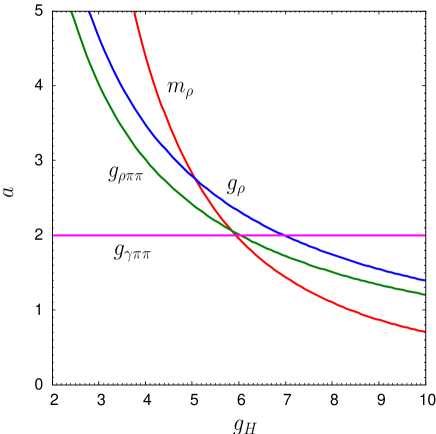
Figure 1: The predictions of the hidden local symmetry. We have used $m_{\rho}=776~{}{\rm MeV}$, $f_{\pi}=92.4~{}{\rm MeV}$, $g_{\rho\pi\pi}=6.03$, $g_{\rho}=(345~{}{\rm MeV})^{2}$, $g_{\gamma\pi\pi}\sim 0$. Values are taken from Ref. [3].

In the unitary gauge, $U_{L}=U_{R}$, the massless pion $\pi^{a}$ is embedded as

$$U_{L}=U_{R}=e^{i\pi^{a}T^{a}/f_{\pi}^{2}}.$$ (6)

The gauge boson $A_{\mu}^{a}$ obtains a mass from the kinetic terms of $U_{L}$ and $U_{R}$. The massive gauge boson describes the $\rho$ meson.

This Lagrangian gives phenomenologically successful nontrivial relations among physical quantities,

$$m_{\rho}^{2}=ag_{H}^{2}f_{\pi}^{2},$$ (7)

$$g_{\rho\pi\pi}={a\over 2}g_{H},$$ (8)

$$g_{\gamma\pi\pi}=-{a-2\over 2}e,$$ (9)

$$g_{\rho}=ag_{H}f_{\pi}^{2}.$$ (10)

These relations are quite successful with

$$g_{H}\simeq 6,\ \ \ a\simeq 2.$$ (11)

The fact that $g_{\gamma\pi\pi}$ vanishes for $a=2$ is called the vector meson dominance and realized in QCD. Fig. 1 demonstrates how successful the model is.

2.2 Linearized hidden local symmetry and the value of $a$

The hidden local symmetry is a non-linear sigma model due to the constraint that $U_{L}$ and $U_{R}$ are unitary matrices. The model can easily be UV completed by embedding $U_{L}$ and $U_{R}$ into some linearly transforming Higgs fields.

For example, $U_{L}$ and $U_{R}$ can be embedded into $q:(N_{f},\overline{N_{f}},1)$ and $\bar{q}:(1,N_{f},\overline{N_{f}})$, respectively. The Lagrangian (the kinetic terms for the Higgs fields) reduces to the hidden local symmetry with $a=1$ at tree level. When one obtains the hidden local symmetry from deconstruction of the extra dimensional gauge theory, this value is realized at the three-site level [21], and becomes $a=4/3$ in the continuum limit [4, 21].

Another example is to include $M:(N_{f},1,\overline{N_{f}})$ in addition to the above model, and embed $U_{L}U_{R}$ to $M$. This reduces to a model with $0<a\leq 1$. The correct sign for the kinetic term of $M$ indicates that $a>1$ is not possible at tree level as one can see in Eq. (1). When we identify $SU(N_{f})_{\rm local}$ as the magnetic gauge theory of SQCD, the Seiberg duality says that the particle content is $q$, $\bar{q}$ and $M$ as the dual quarks and the meson. Therefore, one cannot obtain $a>1$ in the dual picture of the SQCD at tree level. In Ref. [16], it is argued that $a=2$ is realized in SQCD. However, the examples used there is not the chiral symmetry breaking.

Although it sounds unfortunate that the phenomenologically favorable value, $a\sim 2$, cannot be realized in SQCD, we do not argue that the approach from SQCD is unsuccessful. It is important to note that the value $a=2$ is not stable under the renormalization. In Ref. [22], it was found that the $a$ parameter has a UV fixed point at $a=1$. Therefore, having $a\sim 1$ at tree level may not be so bad.

3 An SQCD model as a regularization of QCD

We present a model to study QCD by adding massive modes as regulators. Although it is not guaranteed that the study of such models have something to do with the real QCD, it provides us with qualitative understanding of it if it is smoothly connected to the vacuum of real QCD. We present a model which possesses a sufficiently similar vacuum to the real QCD one.

3.1 Set up

Our goal is to study a non-supersymmetric $SU(N_{c})$ gauge theory with $N_{f}$ massless quarks. We here add various massive modes to make it possible to use the Seiberg duality.

The starting point is an ${\cal N}=1$ supersymmetric $SU(N_{c})$ gauge theory with $N_{f}+N_{c}$ chiral superfields in the fundamental representation. We list the particle content and the quantum numbers in Table 1. Extra $N_{c}$ quarks are added so that the dual gauge group is $SU(N_{f})$.

	$SU(N_{c})$	$SU(N_{f})_{L}$	$SU(N_{f})_{R}$	$U(1)_{B}$	$SU(N_{c})_{V}$	$U(1)_{B^{\prime}}$	$U(1)_{R}$
$Q$	$N_{c}$	$N_{f}$	$1$	1	1	0	$(N_{f}-N_{c})/N_{f}$
$\overline{Q}$	$\overline{N_{c}}$	1	$\overline{N_{f}}$	$-1$	1	0	$(N_{f}-N_{c})/N_{f}$
$Q^{\prime}$	$N_{c}$	1	$1$	0	$\overline{N_{c}}$	1	1
$\overline{Q}^{\prime}$	$\overline{N_{c}}$	1	1	0	${N_{c}}$	$-1$	1

Table 1: Quantum numbers in the electric picture.

In order to remove unwanted modes, first we add a mass term for the extra quarks,

$$W=mQ^{\prime}\bar{Q}^{\prime}.$$ (12)

We also gauge the artificially enhanced $U(1)_{B^{\prime}}$ symmetry so that the breaking of it would not give the Goldstone mode. Finally, we add soft supersymmetry breaking terms to reduce the model to the non-supersymmetric QCD,

$${\cal L}_{\rm soft}=-\tilde{m}^{2}(|Q|^{2}+|\bar{Q}|^{2}+|Q^{\prime}|^{2}+|\bar{Q}^{\prime}|^{2})-\left({m_{\lambda}\over 2}\lambda\lambda+{\rm h.c.}\right)-\left(BmQ^{\prime}\bar{Q}^{\prime}+{\rm h.c.}\right),$$ (13)

where the first and the second terms are the scalar and the gaugino masses, respectively. The last term is the $B$-term associated with the mass term in Eq. (12).

For $N_{f}+N_{c}\leq 3N_{c}/2$, i.e., $N_{f}\leq N_{c}/2$, the dual magnetic picture is a free theory in the IR and thus analysis in the perturbation theory is possible. The use of the Seiberg duality and the perturbative expansions are justified when the mass parameters $m$, $\tilde{m}$, $m_{\lambda}$, and $B$ are all smaller than the dynamical scale. For $N_{c}/2<N_{f}<2N_{c}$, the theory is in the conformal window. The dual description is more weakly coupled for $N_{f}<N_{c}$.

3.2 Magnetic description

	$SU(N_{f})$	$SU(N_{f})_{L}$	$SU(N_{f})_{R}$	$U(1)_{B}$	$SU(N_{c})_{V}$	$U(1)_{B^{\prime}}$	$U(1)_{R}$
$q$	$N_{f}$	$\overline{N_{f}}$	1	0	1	$N_{c}/N_{f}$	$N_{c}/N_{f}$
$\overline{q}$	$\overline{N_{f}}$	1	$N_{f}$	0	1	$-N_{c}/N_{f}$	$N_{c}/N_{f}$
$\Phi$	1	$N_{f}$	$\overline{N_{f}}$	0	1	0	$2(N_{f}-N_{c})/N_{f}$
$q^{\prime}$	$N_{f}$	1	1	1	${{N_{c}}}$	$-(N_{f}-N_{c})/N_{f}$	0
$\overline{q}^{\prime}$	$\overline{N_{f}}$	1	1	$-1$	$\overline{N_{c}}$	$(N_{f}-N_{c})/N_{f}$	0
$Y$	1	1	$1$	0	1 + Adj.	0	2
$Z$	1	1	$\overline{N_{f}}$	$-1$	$\overline{N_{c}}$	1	$(2N_{f}-N_{c})/N_{f}$
$\overline{Z}$	1	$N_{f}$	1	1	${N_{c}}$	$-1$	$(2N_{f}-N_{c})/N_{f}$

Table 2: Quantum numbers in the magnetic picture.

The dual picture is an $SU(N_{f})$ gauge theory as is designed. We would like to identify this gauge theory as the hidden local symmetry. The degrees of freedom in the dual description are mesons $M$ and the dual quarks: $q$, $\bar{q}$, $q^{\prime}$, $\bar{q}^{\prime}$. The quantum numbers are listed in Table 2, where we decomposed the meson as follows:

$$M=\left(\begin{array}[]{cc}Y&Z\\ \bar{Z}&\Phi\\ \end{array}\right).$$ (16)

The superpotential is given by

$$W=m\Lambda Y+h\left(q^{\prime}Y\bar{q}^{\prime}+q^{\prime}Z\bar{q}+q\bar{Z}\bar{q}^{\prime}+q\Phi\bar{q}\right),$$ (17)

where $\Lambda$ is a parameter of the order of the dynamical scale, and $h$ is a dimensionless coupling constant.

At the supersymmetric level, as is well known, the potential has a runaway direction after including the non-perturbative effects, $\langle Y\rangle\neq 0$ and $\langle\Phi\rangle\to\infty$. The dual gauge theory is confined (electric gauge theory is Higgsed). Stabilizing this direction by supersymmetry breaking terms, one can find a vacuum studied in Ref. [18].

As another possibility, $\langle q^{\prime}\bar{q}^{\prime}\rangle\neq 0$ looks minimizing the potential at tree level. Because the rank of $q^{\prime}\bar{q}^{\prime}$ is smaller than $N_{c}$, there is not a stable supersymmetric vacuum in this direction, but there can be a local minimum as in the model of Ref. [23]. The possibility of such a local minimum has been studied in the presence of massless flavors and found that there is not [24]. However, adding supersymmetry breaking terms may create a vacuum. In this case, the dual gauge boson obtains a mass by the $q^{\prime}\bar{q}^{\prime}$ condensation without breaking the $SU(N_{f})_{L}$ $\times$ $SU(N_{f})_{R}$ chiral symmetry. The structure of the hidden local symmetry cannot be seen in this vacuum.

We need to look for other vacua to realize the hidden local symmetry. A good candidate can easily be found by looking at the quantum numbers in Table 2. It is the $q=\bar{q}\neq 0$ direction that breaks chiral symmetry down to the diagonal subgroup and gives a mass for the gauge boson while preserving the baryon number. We now try to find such a minimum by including soft terms in the potential.

3.3 Soft supersymmetry breaking terms in the dual picture

The mapping of the soft supersymmetry breaking terms into the dual theory has been studied in Refs. [25, 26, 27, 28, 29]. In particular, in Ref. [28], simple mapping relations were found between the electric and the magnetic pictures. The soft terms in the dual picture can be parametrized by

$${\cal L}_{\rm soft} = -\tilde{m}_{q}^{2}(|q|^{2}+|\bar{q}|^{2}+|q^{\prime}|^{2}+|\bar{q}^{\prime}|^{2})-\tilde{m}_{M}^{2}(|Y|^{2}+|Z|^{2}+|\bar{Z}|^{2}+|\Phi|^{2})$$ (18)

$$-\left({m_{\tilde{\lambda}}\over 2}{\tilde{\lambda}}{\tilde{\lambda}}+\tilde{B}m\Lambda Y+Ah\left(q^{\prime}Y\bar{q}^{\prime}+q^{\prime}Z\bar{q}+q\bar{Z}\bar{q}^{\prime}+q\Phi\bar{q}\right)+{\rm h.c.}\right).$$

In the free magnetic range, $N_{f}\leq N_{c}/2$, the relations are

$$\tilde{m}^{2}={2N_{c}-N_{f}\over 3(N_{f}+N_{c})}D_{R},$$ (19)

$${m_{\lambda}\over g^{2}}=-{2N_{c}-N_{f}\over 16\pi^{2}}F_{\phi},$$ (20)

$$\tilde{m}_{q}^{2}=-{N_{c}-2N_{f}\over 3(N_{f}+N_{c})}D_{R},$$ (21)

$$\tilde{m}_{M}^{2}={2(N_{c}-2N_{f})\over 3(N_{f}+N_{c})}D_{R},$$ (22)

$${m_{\tilde{\lambda}}\over g_{H}^{2}}=-{2N_{f}-N_{c}\over 16\pi^{2}}F_{\phi},$$ (23)

$$A=2(\gamma_{M}+\gamma_{q}+\gamma_{\bar{q}})F_{\phi},$$ (24)

where $D_{R}$ and $F_{\phi}$ are parameters, and $\gamma_{M}$, $\gamma_{q}$ and $\gamma_{\bar{q}}$ are anomalous dimensions of $M$, $q$ and $\bar{q}$, respectively. The gauge couplings $g$ and $g_{H}$ are those of the electric theory ($SU(N_{c})$) and the magnetic theory ($SU(N_{f})$), respectively.

We should add positive $\tilde{m}^{2}$ in the electric picture. This means $D_{R}>0$. Therefore,

$$\tilde{m}_{q}^{2}<0,\ \ \ \tilde{m}_{M}^{2}>0.$$ (25)

It is interesting to note that $q=q^{\prime}=\bar{q}=\bar{q}^{\prime}=0$ is an unstable point. This indeed triggers the chiral symmetry breaking.

3.4 Hidden local symmetry in the dual theory

The scalar fields have potential from three sources, the $F$-term potential from the superpotential in Eq. (17), the $D$-term from the gauge interactions, and the soft terms in Eq. (18):

$$V=V_{F}+V_{D}+V_{\rm soft}.$$ (26)

The $D$-term potential is given by

$$V_{D} = {g_{H}^{2}\over 2}(q^{\dagger}T^{a}q-\bar{q}T^{a}\bar{q}^{\dagger}+q^{\prime\dagger}T^{a}q^{\prime}-\bar{q}^{\prime}T^{a}\bar{q}^{\prime\dagger})^{2}$$ (27)

$$+{g_{B^{\prime}}^{2}\over 2}\left({N_{c}\over N_{f}}(|q|^{2}-|\bar{q}|^{2})-{N_{f}-N_{c}\over N_{f}}(|q^{\prime}|^{2}-|\bar{q}^{\prime}|^{2})\right)^{2},$$

where $g_{B^{\prime}}$ is the coupling constant of the $U(1)_{B^{\prime}}$ gauge interaction.

Since $Y$ has a linear term and the positive mass squared in Eq. (18), $Y$ can be stabilized at

$$Y=-{\tilde{B}m\Lambda\over\tilde{m}_{M}^{2}}.$$ (28)

Taking $m<B\sim\tilde{m}$ in the electric picture, the VEV of $Y$ is large compared to the soft supersymmetry breaking parameters and can be smaller than $\Lambda$ where the use of duality and weak couplings are justified. With this VEV, the $q^{\prime}$ and $\bar{q}^{\prime}$ obtain supersymmetric mass terms and thus decouple.

Once $q^{\prime}$ and $\bar{q}^{\prime}$ get heavy, the system reduces to a model with $q$, $\bar{q}$, and $\Phi$. This is the linearized hidden local symmetry, or the Landau-Ginzburg model in the magnetic picture. Other light fields, $Y-\langle Y\rangle$, $Z$ and $\bar{Z}$ are not directly coupled to this hidden local sector. Since they are stabilized by the soft terms, one can ignore those fields for the discussion of the vacuum. The fermionic partners of $Z$ and $\bar{Z}$ later obtain masses by the VEV of $q$ and $\bar{q}$. The fermionic component of $Y$ remains massless at tree level. The non-perturbative superpotential, $W\propto(\det M)^{1/N_{f}}$, together with the VEV of $\Phi$ gives a mass to this field.

By minimizing the potential, one can find a vacuum with

$$q=\bar{q}=v{\bf 1}\neq 0,\ \ \ \Phi=v_{\Phi}{\bf 1}\neq 0,$$ (29)

where the chiral symmetry is spontaneously broken and all the gauge bosons obtain masses while, of course, the pions remain massless. In this vacuum, the dual gauge group $SU(N_{f})$ and the diagonal part of the chiral symmetry $SU(N_{f})_{V}\in SU(N_{f})_{L}$ $\times$ $SU(N_{f})_{R}$ is locked, leaving the global $SU(N_{f})_{C+L+R}$ symmetry (the isospin symmetry) unbroken. This is exactly the structure of the hidden local symmetry, where $SU(N_{f})_{\rm local}$ is now identified as the magnetic $SU(N_{f})$ gauge group.

The pion decay constant $f_{\pi}$ and the $a$ parameter are respectively given by

$$f_{\pi}^{2}=2(v^{2}+2v_{\Phi}^{2}),$$ (30)

and

$$a={v^{2}\over v^{2}+2v_{\Phi}^{2}}.$$ (31)

As we know already, $a>1$ cannot be realized in this model.

We show in Figure 2 the parameter region where a stable minimum with the VEVs in Eq. (29) is found. In the figure, we have used a relation $\tilde{m}_{M}^{2}=-2\tilde{m}_{q}^{2}$. When this relation is imposed, the stability of the vacuum requires,

$${\lambda\over\kappa}>{3a^{2}-1\over 2a},\ \ \ {\tilde{\lambda}\over\kappa}>{3a^{2}-1\over 2a},$$ (32)

and

$$3a(1+a)-(3a-1)\sqrt{a(4-3a)}>0.$$ (33)

where

$$\lambda\equiv 2g_{B^{\prime}}^{2}\left(N_{c}\over N_{f}\right)^{2},\ \ \ \tilde{\lambda}\equiv{g_{H}^{2}\over N_{f}},\ \ \ \kappa\equiv{h^{2}\over N_{f}}.$$ (34)

Eq. (33) gives $a>0.124$. When $\tilde{m}_{q}^{2}<0$ is further imposed, we find a stronger constraint

$$a>{1\over 3}.$$ (35)

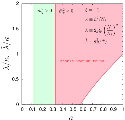
Figure 2: Region where a stable vacuum with chiral symmetry breaking is found.

The vacuum exists even in the limit where the $U(1)_{B^{\prime}}$ gauge interaction is extremely weak. This means that a scale where the $U(1)_{B^{\prime}}$ gauge coupling hits the Landau pole can be arbitrarily high, that we want to be at least higher than the dynamical scale $\Lambda$ for the model to be well-defined. Therefore, one can freely take very small mass parameters so that all the interactions are weak at the scale of $f_{\pi}$, and thus the analysis at tree level is reliable. We now have established the presence of the vacuum in Eq. (29) in the weakly coupled regime. The vacuum has the same structure of the hidden local symmetry where the chiral symmetry is spontaneously broken. The $\rho$ meson is identified as the magnetic gauge boson. Its mass prevents a magnetic flux of $SU(N_{f})$ to enter the vacuum, describing the confinement in the electric picture if the Seiberg duality is the electric-magnetic duality. The fermion components of $q$, $\bar{q}$, and $\Phi$ all obtain masses when $a\neq 0,1$.

Weinberg and Witten have shown that the massless gauge boson cannot be created by the global current [30]. Our $\rho$ meson as the magnetic gauge boson may sound contradicting to this theorem since the $\rho$ meson couples to the flavor current. However, the $\rho$ meson in our framework couples to the global current only after the dual color-flavor locking. Therefore, at the massless point, the dual color and the flavor symmetry is not related, and thus the $\rho$ meson does not couple to the global current in the massless limit.

4 QCD case ($N_{c}=3$, $N_{f}=2$)

In the following we try to see if how well the vaccum found in the previous section describes the hadron world in real QCD. Most of the discussions are qualitative and sometimes speculative, but we can provide new interpretations of the nature of hadrons.

4.1 Light mesons as magnetic degrees of freedom

Since the model, supersymmetric $SU(3)$ gauge theory with $N_{f}+N_{c}=5$ flavors, is in the conformal window, we cannot take the weakly coupled limit in the infrared. Nevertheless, one can argue that the dual picture is still more weakly coupled compared to the electric one. In the regime of the conformal field theory, anomalous dimensions of $q$, $\bar{q}$, and $\Phi$ fields are, respectively, $-1/10$, $-1/10$ and $1/5$, which may be small enough to justify the expansion in terms of those fields around the free theory.

In the conformal window, the predictions for the soft parameters are different from the free magnetic case. In fact, the soft terms (except for the $\tilde{B}$ term) approach to zero if the hierarchy of the dynamical scale and the mass parameters ($m$ and soft terms) is large enough. However, when we discuss applications to phenomenology, we are interested in the case with no hierarchy where there is no prediction on the size or relations among supersymmetry breaking terms. We, therefore, treat them as free parameters for the analysis.

The boson sector of the model contains various massive and massless modes. We propose to identify them as light mesons in QCD. In addition to the massless Nambu-Goldstone particles, $\pi$ (and $\eta$ at this stage), our model contains massive modes:

• $\rho(770)$ as the magnetic gauge boson,

• $\omega(782)$ as the $U(1)_{B^{\prime}}$ gauge boson,

• $f_{0}(600)$, $f_{0}(980)$, $f_{0}(1370)$ as the CP-even trace parts of $q$, $\bar{q}$ and $\Phi$,

• $\eta(1295)$ as the uneaten CP-odd trace part of $q$, $\bar{q}$ and $\Phi$,

• $a_{0}(?)$, $a_{0}(980)$, $a_{0}(1450)$ as the CP-even traceless parts of $q$, $\bar{q}$ and $\Phi$, and

• $\pi(1300)$ as the uneaten CP-odd traceless part of $q$, $\bar{q}$ and $\Phi$.

There should be three CP-even isospin-triplet scalars (called $a_{0}$) as mixtures of $q$, $\bar{q}$ and $\Phi$. We could not find one of them in the table in [31].

In the potential, there are numbers of parameters:

$$f_{\pi}^{2},\ \ \ a,\ \ \ g_{H},\ \ \ g_{B^{\prime}},\ \ \ h,\ \ \ \xi={\tilde{m}_{M}^{2}\over\tilde{m}_{q}^{2}}.$$ (36)

It is probably not very meaningful to try to fit the hadron spectrum with those parameters since we already know that the phenomenologically favorable value, $a\sim 2$, cannot be obtained at tree level. However, from the special shape of the potential, one can find sum rules independent of parameters:

$$\sum_{i=1}^{3}m_{f_{0,i}}^{2}=m_{\eta_{H}}^{2}+m_{\omega}^{2},$$ (37)

$$\sum_{i=1}^{3}m_{a_{0,i}}^{2}=m_{\pi_{H}}^{2}+m_{\rho}^{2},$$ (38)

$$m_{\eta_{H}}^{2}=m_{\pi_{H}}^{2},$$ (39)

where $f_{0,i}$ ($a_{0,i}$) are the three mass eigenstates corresponding to mixtures of three CP-even isospin singlet (triplet) part of $q$, $\bar{q}$, and $\Phi$, and $\eta_{H}$ and $\pi_{H}$ are massive states of the CP-odd isospin singlet and triplet scalars, respectively. The sum rule in Eq. (37) can be tested by inputting masses listed above. The agreement is at the level of $40\%$, which we think is good enough since we expect a quantum correction of $O(g_{H}^{2}N_{f}/(4\pi)^{2})$, non-perturbative effects, and also corrections from finite quark masses which we discuss later. The second sum rule in Eq. (38) cannot be tested since we could not find three $a_{0}$’s in the hadron spectrum. The sum rule suggest that the missing one is very light. The third one in Eq. (39) agrees very well although it is not surprising from the view point of the quark model.

We have so far ignored the finite masses for the quarks. The effects of the finite quark mass can be taken into account by adding a mass term $m_{Q}Q\bar{Q}$ in the superpotential in the electric picture. In the magnetic picture, this mass term induces a linear term of the meson,

$$W_{\rm mass}=m_{Q}\Lambda\Phi,$$ (40)

which explicitly breaks the chiral symmetry. The pions obtain masses from this term.

4.2 $\eta$

At the classical level in the dual theory, $\eta$ (it is $\eta^{\prime}$ in the three flavor language) is massless, but it can obtain a mass through non-perturbative superpotential. In a meson direction where the dual squarks can be integrated out, there is a non-perturbative superpotential,

$$W_{\rm dyn}\propto\left({\rm det}M\right)^{1/N_{f}}.$$ (41)

Since this term explicitly breaks the anomalous $U(1)$ axial symmetry, $\eta$ obtains a mass. The size is suppressed by a factor of

$$e^{-{8\pi^{2}/(g_{H}^{2}N_{f})}}$$ (42)

compared to the scale of the $\rho$ meson mass. This is not quite a suppression factor when we input $g_{H}\sim 6$, and thus one can only make a qualitative argument.

The above superpotential is generated by the non-perturbative effect, such as the instanton configurations of the $\rho$ meson. In this view, the $\rho$ meson is responsible for the solution to the $U(1)$ problem.

4.3 QCD string?

There is a stable string configuration associated with the spontaneous $U(1)_{B^{\prime}}$ breaking by the VEVs of the dual squarks. This type of string has been discussed in Refs. [32, 33, 13, 15, 34] where its connection to confinement has been emphasized. The string solution involves the non-trivial configurations of the $SU(N_{f})$ gauge fields as well as $U(1)_{B^{\prime}}$. The solution is called a non-abelian vortex string as it non-trivially transforms under the unbroken $SU(N_{f})_{C+L+R}$ isospin symmetry. The string carries the non-abelian magnetic flux (which is the color flux in the electric picture), and thus can be interpreted as the QCD string. It is amusing that the non-trivial configurations of the $\rho$ and $\omega$ mesons can be interpreted as the QCD string! The QCD string is a singularity in the vacuum at which $\rho$ and $\omega$ become massless [8] and thus allows the color flux to penetrate.

The QCD string should be unstable in the presence of the quarks. In order to describe the instability at the length scale of ${\cal O}(\Lambda_{\rm QCD}^{-1})$, one probably needs a larger framework which explains the nature of $U(1)_{B^{\prime}}$ and extra flavors. For example, the meta-stable string and its connection to color confinement has been discussed in the softly broken ${\cal N}=2$ theory in Ref. [12] where a $U(1)$ factor originates from a breaking of the $SU(N)$ gauge group.

4.4 Constituent quarks?

Figure 3: Quiver diagram of the model.

It is interesting to note that the fermionic components of $Z$, $\bar{Z}$, $q^{\prime}$ and $\bar{q}^{\prime}$ have the quantum numbers of quarks if we gauge the $SU(N_{c})_{V}$ global symmetry. This gauging is a natural procedure since the global symmetry is an artificially enhanced one by the introduction of the extra quarks. The dual quarks $q^{\prime}$ and $\bar{q}^{\prime}$ obtain masses by the VEV of $Y$. In the language of the hidden local symmetry sketched in Figure 3, those are matter fields living in the middle site. The fields living in the left and right site, $Z$ and $\bar{Z}$, obtain masses through the mixing with $q^{\prime}$ and $\bar{q}^{\prime}$ induced by the chiral symmetry breaking ($\langle q\rangle=\langle\bar{q}\rangle\neq 0$). These massive “quarks” in the dual picture can naturally be identified as the constituent quarks in the quark model.

However, these “quarks” cannot be the endpoints of the string we discussed above. The string solution carries the magnetic flux of $U(1)_{B^{\prime}}$ whereas the “quarks” only have electric charges. Again, we probably need a larger framework to understand the whole picture.

4.5 Baryons

There are a few ways to describe baryons in this model. The simplest one is to introduce a massive vector-like pair of fermions which transform as fundamental and anti-fundamental under the $SU(N_{f})$ dual gauge group (the middle site in Figure 3). Since they are massive, one can assume that those are lost in passing through the Seiberg duality. In this case, the baryons are flavor singlet and massive in the chiral symmetric phase, but after the (dual) color-flavor locking by the VEV of $q$ and $\bar{q}$, the fermions carry the same quantum numbers as the proton and the neutron.

Another way is to argue that the skyrmion solution describes the baryons [35]. In the above two cases, one can explain the universality of the $\rho$ meson couplings, $g_{\rho NN}=g_{H}$, which was not automatic in the hidden local symmetry [35, 36].

Of course, the baryons can be three-quark states made of the constituent quarks we found above. However, in this case, the coupling universality is not automatic. The coupling depends on the mixing between $q^{\prime}$ and $Z$ and also on how baryons are composed of.

5 Application to electroweak symmetry breaking

The electroweak symmetry breaking in the standard model has the same structure as chiral symmetry breaking in QCD once we embed the $SU(2)_{L}$ $\times$ $U(1)_{Y}$ gauge group into the global symmetry, $SU(N_{f})_{L}$ $\times$ $SU(N_{f})_{R}$. The SQCD model can be thought of as a deformation of the QCD-like technicolor theory where we have a weakly coupled description.

For concreteness, we take the model with $N_{c}=3$ and $N_{f}=2$, and weakly gauge $SU(N_{f})_{L}$ which is identified as $SU(2)_{L}$ of the weak interaction. We embed the $U(1)_{Y}$ group as $T_{3}$ generator of the $SU(N_{f})_{R}$. By this embedding, one can notice that the meson field $\Phi$ has the same quantum numbers as the Higgs field and its conjugate, $\Phi=(H,\tilde{H})$. The model with $N_{c}=3$ and $N_{f}=2$ is in the conformal window, and the Higgs field has an anomalous dimension $1/5$. This model provides us with an almost elementary Higgs field, and thus phenomenologically friendly [37].

The $S$ parameter [38] can be calculated by using the magnetic picture. There is a tree level contribution to the $S$ parameter from the exchange of the $\rho$ meson. This contribution is

$$\Delta S=4\pi\cdot{g_{\rho}^{2}\over m_{\rho}^{4}}={4\pi\over g_{H}^{2}},$$ (43)

which is independent of the $a$ parameter. If we put $g_{H}=6$ as an estimate motivated by QCD, we obtain $\Delta S\sim 0.3$. This is quite big. However, given that there is a Higgs boson, the situation is slightly better compared to the QCD-like technicolor theories if the Higgs boson is light enough.

References

- [1] M. Bando, T. Kugo, S. Uehara, K. Yamawaki, T. Yanagida, Phys. Rev. Lett. 54, 1215 (1985).
- [2] T. Sakai, S. Sugimoto, Prog. Theor. Phys. 113, 843-882 (2005). [arXiv:hep-th/0412141 [hep-th]].
- [3] J. Erlich, E. Katz, D. T. Son, M. A. Stephanov, Phys. Rev. Lett. 95, 261602 (2005). [hep-ph/0501128].
- [4] L. Da Rold, A. Pomarol, Nucl. Phys. B721, 79-97 (2005). [hep-ph/0501218].
- [5] M. J. Strassler, Prog. Theor. Phys. Suppl. 131, 439 (1998) [arXiv:hep-lat/9803009].
- [6] N. Seiberg, E. Witten, Nucl. Phys. B426, 19-52 (1994). [hep-th/9407087].
- [7] N. Seiberg, E. Witten, Nucl. Phys. B431, 484-550 (1994). [hep-th/9408099].
- [8] G. ’t Hooft, Nucl. Phys. B190, 455 (1981).
- [9] S. Mandelstam, Phys. Lett. B53, 476-478 (1975).
- [10] G. Carlino, K. Konishi, H. Murayama, JHEP 0002, 004 (2000). [hep-th/0001036]; G. Carlino, K. Konishi, H. Murayama, Nucl. Phys. B590, 37-122 (2000). [hep-th/0005076]; G. Carlino, K. Konishi, S. Prem Kumar, H. Murayama, Nucl. Phys. B608, 51-102 (2001). [hep-th/0104064].
- [11] K. Konishi, G. Marmorini, N. Yokoi, Nucl. Phys. B741, 180-198 (2006). [hep-th/0511121].
- [12] M. Eto, L. Ferretti, K. Konishi, G. Marmorini, M. Nitta, K. Ohashi, W. Vinci, N. Yokoi, Nucl. Phys. B780, 161-187 (2007). [hep-th/0611313].
- [13] A. Gorsky, M. Shifman, A. Yung, Phys. Rev. D75, 065032 (2007). [hep-th/0701040].
- [14] N. Seiberg, Nucl. Phys. B435, 129-146 (1995). [hep-th/9411149].
- [15] M. Shifman, A. Yung, Phys. Rev. D76, 045005 (2007). [arXiv:0705.3811 [hep-th]]; M. Shifman, A. Yung, Phys. Rev. D83, 105021 (2011). [arXiv:1103.3471 [hep-th]].
- [16] Z. Komargodski, JHEP 1102, 019 (2011). [arXiv:1010.4105 [hep-th]].
- [17] M. Harada, K. Yamawaki, Phys. Rev. Lett. 83, 3374-3377 (1999). [hep-ph/9906445].
- [18] O. Aharony, J. Sonnenschein, M. E. Peskin, S. Yankielowicz, Phys. Rev. D52, 6157-6174 (1995). [hep-th/9507013].
- [19] N. Seiberg, Phys. Rev. D49, 6857-6863 (1994). [hep-th/9402044].
- [20] S. P. Martin, J. D. Wells, Phys. Rev. D58, 115013 (1998). [hep-th/9801157].
- [21] A. S. Belyaev, R. Sekhar Chivukula, N. D. Christensen, H. -J. He, M. Kurachi, E. H. Simmons, M. Tanabashi, Phys. Rev. D80, 055022 (2009). [arXiv:0907.2662 [hep-ph]].
- [22] M. Harada, K. Yamawaki, Phys. Lett. B297, 151-158 (1992). [hep-ph/9210208].
- [23] K. A. Intriligator, N. Seiberg, D. Shih, JHEP 0604, 021 (2006). [hep-th/0602239].
- [24] A. Giveon, A. Katz and Z. Komargodski, JHEP 0806, 003 (2008) [arXiv:0804.1805 [hep-th]].
- [25] H. -C. Cheng, Y. Shadmi, Nucl. Phys. B531, 125-150 (1998). [hep-th/9801146].
- [26] N. Arkani-Hamed, R. Rattazzi, Phys. Lett. B454, 290-296 (1999). [hep-th/9804068].
- [27] A. Karch, T. Kobayashi, J. Kubo, G. Zoupanos, Phys. Lett. B441, 235-242 (1998). [hep-th/9808178].
- [28] M. A. Luty, R. Rattazzi, JHEP 9911, 001 (1999). [hep-th/9908085].
- [29] S. Abel, M. Buican, Z. Komargodski, Phys. Rev. D84, 045005 (2011). [arXiv:1105.2885 [hep-th]].
- [30] S. Weinberg, E. Witten, Phys. Lett. B96, 59 (1980).
- [31] K. Nakamura et al. [ Particle Data Group Collaboration ], J. Phys. G G37, 075021 (2010).
- [32] A. Hanany, D. Tong, JHEP 0307, 037 (2003). [hep-th/0306150].
- [33] R. Auzzi, S. Bolognesi, J. Evslin, K. Konishi, A. Yung, Nucl. Phys. B673, 187-216 (2003). [hep-th/0307287].
- [34] M. Eto, K. Hashimoto, S. Terashima, JHEP 0709, 036 (2007). [arXiv:0706.2005 [hep-th]].
- [35] T. Fujiwara, Y. Igarashi, A. Kobayashi, H. Otsu, T. Sato, S. Sawada, Prog. Theor. Phys. 74, 128 (1985).
- [36] M. Bando, T. Kugo, K. Yamawaki, Prog. Theor. Phys. 73, 1541 (1985).
- [37] H. Fukushima, R. Kitano, M. Yamaguchi, JHEP 1101, 111 (2011). [arXiv:1012.5394 [hep-ph]].
- [38] M. E. Peskin, T. Takeuchi, Phys. Rev. Lett. 65, 964-967 (1990); Phys. Rev. D46, 381-409 (1992).