Condensate fraction in liquid ⁴He at zero temperature

Abstract

We present results of the one-body density matrix $\rho_{1}(r)$ and the condensate fraction $n_{0}$ of liquid ⁴He calculated at zero temperature by means of the Path Integral Ground State Monte Carlo method. This technique allows to generate a highly accurate approximation for the ground state wave function $\Psi_{0}$ in a totally model-independent way, that depends only on the Hamiltonian of the system and on the symmetry properties of $\Psi_{0}$. With this unbiased estimation of $\rho_{1}(r)$, we obtain precise results for the condensate fraction $n_{0}$ and the kinetic energy $K$ of the system. The dependence of $n_{0}$ with the pressure shows an excellent agreement of our results with recent experimental measurements. Above the melting pressure, overpressurized liquid ⁴He shows a small condensate fraction that has dropped to $0.8\%$ at the highest pressure of $p=87\,{\rm bar}$.
keywords: Liquid Helium, Bose-Einstein condensation, Quantum Monte Carlo.

I Introduction

Several microscopic theories point out that the phenomenon of superfluidity in liquid ⁴He has to be seen as a consequence of Bose-Einstein condensation (BEC).¹ Having total spin $S=0$, ⁴He atoms behave like bosons and, below the critical temperature $T_{\lambda}=2.17\,{\rm K}$, they can occupy macroscopically the same single-particle state. Nevertheless, the strong interaction between ⁴He atoms does not allow all of them to occupy the lowest energy state and, even at zero temperature, only a small fraction $n_{0}=N_{0}/N$ of the $N$ particles is in the condensate.

The macroscopic occupation of the lowest energy state, in a strongly correlated system like ⁴He, appears in the momentum distribution $n(\bf{k})$ as a delta-peak at $\bf{k}=0$ and a divergent behavior $n(k)\sim 1/k$ when $k\to 0$. In the coordinate space, the presence of BEC in a homogeneous system can be deduced from the asymptotic behavior of the one-body density matrix $\rho_{1}(\bf{r})$ ($n_{0}=\lim_{r\to\infty}\rho_{1}(r)$), which is the inverse Fourier transform of $n(\bf{k})$.

Experimental estimates of $n_{0}$ can be obtained from the dynamic structure factor, $S(q,\omega)$, measured by neutron inelastic scattering at high energy and momentum transfer. These measurements have a long history:^{2, 3, 4} in the 80s, the first experiments gave estimates for $n_{0}$ slightly above 10%, but they were affected by a poor instrumental resolution and by some difficulties in describing the final states effects of the scattering experiment. Recently, with the advances in the experimental technology and in the method of analysis of the scattering data, Glyde et al.⁵ have been able to give improved estimations of $n_{0}$ at very low temperature. At saturated vapor pressure (SVP), they found $n_{0}=(7.25\pm 0.75)\%$,⁵ and more recently they have measured the dependence of $n_{0}$ with pressure $p$.⁶

Because of the strong correlations between ⁴He atoms, the calculation of the one-body density matrix in superfluid ⁴He cannot be obtained analytically via a perturbative approach. It is necessary the use of microscopic simulations to provide accurate estimations of the condensate fraction. In particular, the Path Integral Monte Carlo (PIMC) method has been widely used in the study of ⁴He at finite temperature, thanks to its capability of furnishing in principle exact numerical estimates of physical observables relying only on the Hamiltonian of the system.⁷ The first calculations of $n_{0}$ with this method date back to 1987,⁸ but most recent simulations based on an improved sampling algorithm provide very accurate results for $\rho_{1}(r)$, showing a condensate fraction $n_{0}=0.081\pm 0.002$ at temperature $T=1\,{\rm K}$. ⁹ At zero temperature, ground-state projection techniques are widely used in the study of BEC properties of ⁴He. Diffusion Monte Carlo technique, for instance, has provided estimations of $n_{0}$ in liquid ⁴He on a wide range of pressures.^{10, 11, 12} This method, however, suffers from the choice of a variational ansatz necessary for the importance sampling whose influence on $\rho_{1}(r)$ cannot be completely removed. Reptation Quantum Monte Carlo (RQMC) has also been used for this purpose,¹³ but the calculated value of $n_{0}$ at SVP lies somewhat below the recent PIMC value ⁹ at $T=1\,{\rm K}$ noted above.

Motivated by recent accurate experimental data on $n_{0}(p)$, our aim in the present work is to perform new calculations of $\rho_{1}(r)$ and of $n_{0}$ in liquid ⁴He at zero temperature using a completely model-independent technique based on path integral formalism. The Path Integral Ground State (PIGS) Monte Carlo method is able to compute exact quantum averages of physical observables without importance sampling, that is without taking into account any a priori trial wave function.¹⁴ Using a good sampling scheme in our Monte Carlo simulations, we are able to provide very precise calculations of the one-body density matrix at different densities. We fit our numerical data for $\rho_{1}(r)$ with the model used in previous experimental works, ⁵ highlighting the merits and the faults of this model, and finally we give our estimations for the condensate fraction when changing the pressure of the liquid, showing an excellent agreement with experimental data.⁶

The PIGS method and the computational details of our simulation are discussed in Sec. II. The results are presented in Sec. III and Sec. IV comprises the main conclusions.

II The PIGS method

The PIGS approach to the study of quantum systems consists in a systematic improvement of a trial wave function $\Psi_{T}$ by repeated application of the evolution operator in imaginary time, which eventually drives the system into the ground state,¹⁵ according to the formula

$$\Psi_{PIGS}(R_{M})=\int\prod_{i=1}^{M}dR_{i-1}G(R_{i},R_{i-1};\tau)\Psi_{T}(R_{0})\ ,$$ (1)

where the $R_{i}=\{{\bf r}_{i;1},{\bf r}_{i;2},...,{\bf r}_{i;N}\}$ represent different sets of coordinates the $N$ particles of the system, and $G(R^{\prime},R;\tau)=\langle R^{\prime}|e^{-\tau\hat{H}}|R\rangle$ is the imaginary time propagator.

Given an approximation of $G(R,R^{\prime};\tau)$ for small $\tau$, the averages of diagonal observables can be calculated mapping the quantum many-body system onto a classical system made up of $N$ interacting polymers composed by $2M+1$ beads, each of them representing a different evolution in imaginary time of the initial trial state $\Psi_{T}$. Increasing the number $M$, one is able to reduce the systematic error and therefore to recover ”exactly” the ground-state properties of the system.

A good approximation for the propagator $G$ is important for improving the numerical efficiency of the method: this greatly reduces the complexity of the calculation and ergodicity issues, allowing to simulate the quantum system with few beads, each one with a large time step. Using a high-order approximation for the propagator, it is possible to obtain an accurate description of the exact ground state wave function with little numeric effort, even when the initial trial wave function contains no more information than the bosonic statistics, that is when one starts the imaginary time evolution from $\Psi_{T}=1$.¹⁶

The one-body density matrix can be written as

$$\rho_{1}({\bf r}_{1},{\bf r^{\prime}}_{1})=\frac{\int d{\bf r}_{2}...d{\bf r}_{N}\Psi^{*}_{0}(R)\Psi_{0}(R^{\prime})}{\int d{\bf r}_{1}...d{\bf r}_{N}|\Psi_{0}(R)|^{2}}\ ,$$ (2)

where the configuration $R=\{{\bf r}_{1},{\bf r}_{2},...,{\bf r}_{N}\}$ differs from $R^{\prime}=\{{\bf r^{\prime}}_{1},{\bf r}_{2},...,{\bf r}_{N}\}$ only by the position of one of the $N$ atoms. In the PIGS approach, the expectation value of non-diagonal observables, like $\rho_{1}$, is computed mapping the quantum system in the same classical system of polymers as in the diagonal case, but cutting one of these polymers in the mid point. Building the histogram of the frequencies of the distances between the cut extremities of the two half polymers, one can compute the numerator in Eq. (2). The calculation of the normalization factor at the denominator is not strictly necessary since the histogram can be normalized imposing the condition $\rho_{1}(0)=1$. However, this a posteriori normalization procedure is not easy, because of the small occurrences of the distances close to zero, and may introduce systematic errors in the estimation of the condensate fraction $n_{0}$. In our work, we have avoided this problem incorporating in the sampling the worm algorithm (WA), a technique previously developed for path integral Monte Carlo simulations at finite temperature.⁹ The key aspect of WA is to work in an extended configuration space, containing both diagonal (all polymers with the same length) and off-diagonal (one polymer cut in two separate halves) configurations, and one of its main advantages is its capability of evaluating the normalization factor in off-diagonal estimators. We have extended this technique to zero-temperature calculations and we have been able to get automatically the properly normalized $\rho_{1}$, and therefore very precise estimations of $n_{0}$. In our simulations, the sampling also contains movements involving the principle of indistinguishability of quantum particles, like the swap update ⁹. Even though swaps are not strictly necessary since boson symmetry is fulfilled with a proper choice of the imaginary time propagator, they improve the sampling allowing a larger displacement of the half polymers and thus a better exploration of the long range limit of $\rho_{1}$.

III Results

To compute $\rho_{1}(r)=\rho_{1}(|{\bf r}_{1}-{\bf r^{\prime}}_{1}|)$ in liquid ⁴He at several densities, we have carried out different simulations with a cubic box with periodic boundary conditions containing $N=128$ atoms interacting through the Aziz pair potential.¹⁷ At first we study the system at the equilibrium density $\rho=0.02186\,$ Å^-3: our result for $\rho_{1}(r)$ is shown in Fig. 1. We have checked that our results starting with $\Psi_{T}=1$ or with a Jastrow-McMillan wave function are statistically indistinguishable. In order to check how the finite size of the box affects our results, we have performed a simulation of the same system in a larger box containing $N=256$ ⁴He atoms. In Fig. 1, we have compared $\rho_{1}(r)$ obtained in this last simulation with the one estimated using a smaller number of particles: we can see that, up to the distances reachable with the smaller system, these two results agree within the statistical error. Furthermore, the two functions reach the same plateau at the largest available distances, indicating that the asymptotic regime for $\rho_{1}(r)$ is already achieved using $N=128$ ⁴He atoms.

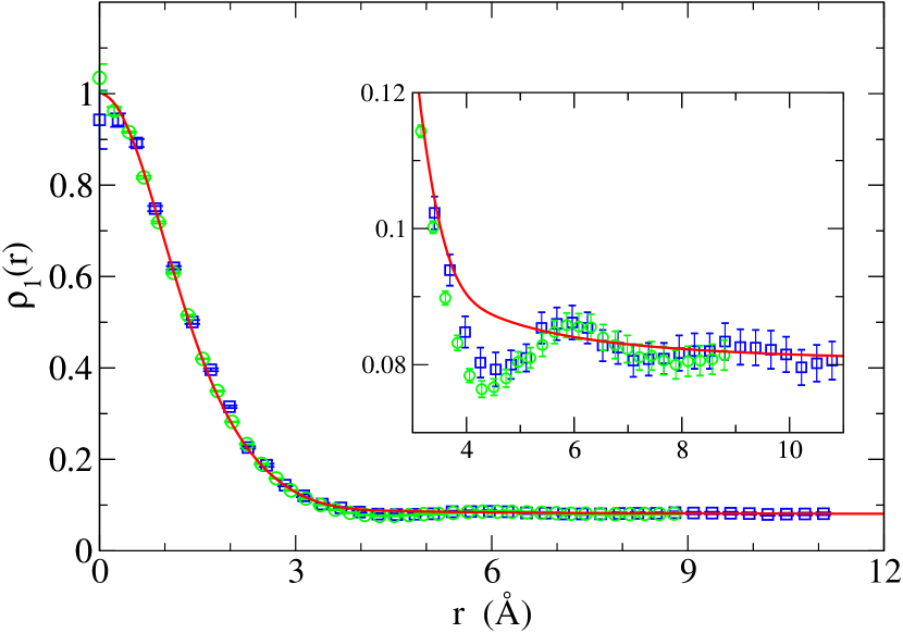
Figure 1: (Color online) One-body density matrix $\rho_{1}(r)$ at the equilibrium density $\rho=0.02186$ Å^-3. The symbols represents the result of the PIGS simulations for the system containing $N=128$ (green circles) and $N=256$ (blue squares) ⁴He atoms. The red line is the curve obtained fitting these data with Eq. 3 with optimal values: $k_{c}=1.369\pm 0.020\ \textrm{\AA}^{-1}$, $\alpha_{2}=0.794\pm 0.005\ \textrm{\AA}^{-2}$, $\alpha_{4}=0.355\pm 0.050\ \textrm{\AA}^{-4}$, $\alpha_{6}=0.680\pm 0.080\ \textrm{\AA}^{-6}$, and $n_{0}=0.0801\pm 0.0022$. The inset shows the same data for $r$ between 3 Åand 11 Åon an expanded scale.

To fit our data we use the model proposed by Glyde in Ref. ² that has been used in the analysis of experimental data,⁵

$$\rho_{1}(r)=n_{0}[1+f(r)]+A\rho_{1}^{*}(r)\ .$$ (3)

The function $f(r)$ represents the coupling between the condensate and the non-zero momentum states. In momentum space, one can express $f(k)$ in terms of the phonon response function ²,

$$f(k)=\left[\frac{mc}{2\hbar(2\pi)^{3}\rho}\frac{1}{k}\coth\left(\frac{c\hbar k}{2k_{B}T}\right)\right]e^{-k^{2}/(2k_{c}^{2})}\ ,$$ (4)

with $c$ the speed of sound. Since we work in the coordinate space, we are interested in its 3D Fourier transform $f(r)$, which at zero temperature can be written as

$$f(r)=\frac{mc}{\hbar(2\pi)^{2}\rho}\frac{\sqrt{2}k_{c}}{r}D\left(\frac{k_{c}r}{\sqrt{2}}\right)\ ,$$ (5)

where $D(x)=e^{-x^{2}}\int_{0}^{x}{dte^{t^{2}}}$ is the Dawson function. To describe the contribution to $\rho_{1}$ from the states above the condensate, which we denote by $\rho_{1}^{*}$, we use the cumulant expansion of the intermediate scattering function, that is the Fourier Transform of the longitudinal momentum distribution,²

$$\rho_{1}^{*}(r)=\exp\left[-\frac{\alpha_{2}r^{2}}{2!}+\frac{\alpha_{4}r^{4}}{4!}-\frac{\alpha_{6}r^{6}}{6!}\right]\ .$$ (6)

The constant $A$ appearing in Eq. (3) is fixed by the normalization condition $\rho_{1}(0)=1$. Therefore, the model we used has five parameters: $n_{0}$, $k_{c}$, $\alpha_{2}$, $\alpha_{4}$ and $\alpha_{6}$. It has to be noticed that, unlike what is done in the treatment of the experimental data, where $k_{c}$ is chosen as a cut-off parameter to make the term $f(k)$ vanish out of the phonon region, we have considered $k_{c}$ as a free parameter of the fit.

The best fit we get using the model of Eq. (3) is shown in Fig. 1. This model is able to reproduce the behavior of $\rho_{1}(r)$ for short distances and in the asymptotic regime, but cannot describe well the numerical data in the range of intermediate $r$. Indeed, for distances above 3 Å, $\rho_{1}(r)$ obtained with PIGS presents oscillations which are damped at larger $r$, as observed also in previous theoretical calculations.^{13, 9} This non monotonic behavior, which can be attributed to coordination shell oscillations,⁹ is difficult to describe within the model of Eq. 3.

Nevertheless, despite of these difficulties in describing the oscillations of the $\rho_{1}(r)$ obtained with PIGS, the fit we gave using the model of Eq. (3) contains important informations about the ground state of liquid ⁴He. First of all, from the long range behavior, we can obtain the value of the condensate fraction $n_{0}$. From our analysis, we get $n_{0}=0.0801\pm 0.0022$, in complete agreement with the value $n_{0}=0.081\pm 0.002$ obtained by Boninsegni et al.⁹ in a path integral Monte Carlo simulation at temperature $T=1\,{\rm K}$, and in good agreement with the experimental result $n_{0}=0.0725\pm 0.0075$.⁵ Furthermore, from the behavior of $\rho_{1}(r)$ at short distances, we can obtain an estimation of the kinetic energy per particle $K/N$. In particular, the term $\alpha_{2}$ appearing in Eq. (6) is the second moment of the struck atom wave vector projected along the direction of the incoming neutron ² and is related to the kinetic energy per particle by the formula $K/N=3(\hbar^{2}/2m)\alpha_{2}$. Using the value $\alpha_{2}=(0.794\pm 0.005)$ Å^-2 obtained in our fit, we get $K/N=(14.43\pm 0.09)\,{\rm K}$ which has to be compared with the value obtained in the PIGS simulation, $K/N=(14.37\pm 0.03)\,{\rm K}$.

In Fig. 2, we show results of $n(k)$ obtained performing a numerical Fourier transform of $\rho_{1}(r)$ and we compare it with the Fourier transform of Eq. 3,

$$n(k)=n_{0}\delta(k)+n_{0}f(k)+An^{*}(k)\ .$$ (7)

The PIGS data are plotted from $k_{min}=2\pi/L\simeq 0.4\,$ Å^-1 , $L$ being the length of the simulation box, and are not able to reproduce the $1/k$ behavior of $n(k)$ at low $k$ because of finite size effects; for $k>k_{min}$ the effect of $f(k)$ vanishes and $n(k)=n^{*}(k)$. We notice that the disagreement between the two curves is larger in the region between $k\simeq 1\,$ Å^-1 and $k\simeq 2.5\,$ Å^-1. In this range, indeed, $n(k)$ obtained with the PIGS method presents a change of curvature, not seen in $n(k)$ obtained from the fit.

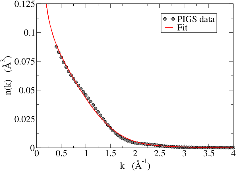
Figure 2: (Color online) The momentum distribution $n(k)$ at equilibrium density $\rho=0.02186$ Å^-3: the black circles represents the numerical result obtained from the PIGS simulation, the red line represents the FT of the fit for $\rho_{1}(r)$ obtained according to Eq. (3).

This discrepancy can be explained considering the coupling between the condensate and the states out of it. The term $f(k)$, defined in Eq. (4), is obtained considering only pure density excitations in the system and, therefore, is valid only in the limit of small momenta.² At higher $k$, one should consider even the contributions due to the coupling of the condensate to the excited states out of the phonon region. However, little is known about these contributions and it is difficult to include them in a more complete form for $f(k)$ in order to give a more reliable model for the momentum distribution.

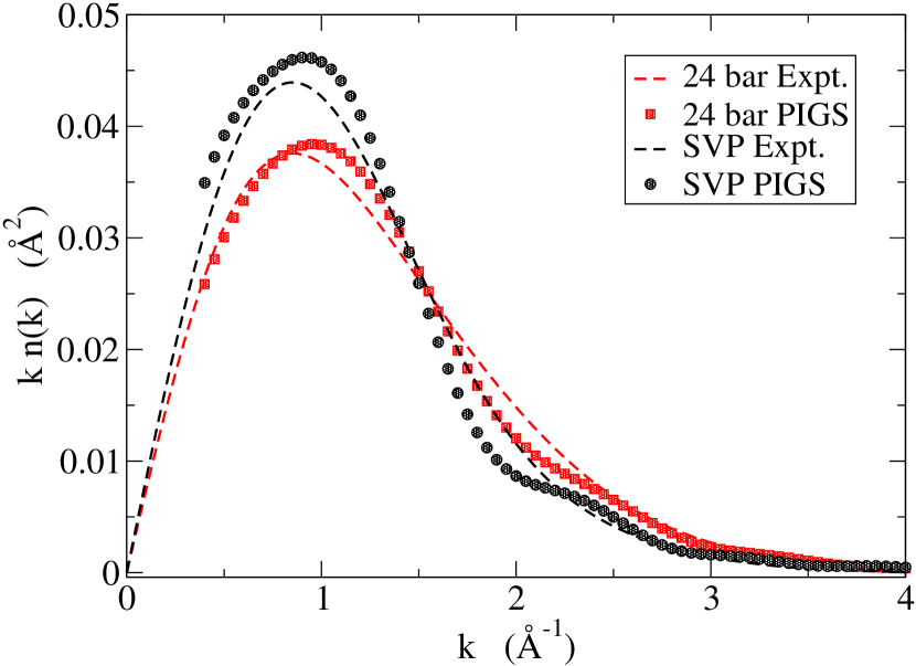
Figure 3: (Color online) The momentum distribution, plotted as $kn(k)$, in liquid ⁴He at two different pressure: black circles and red squares are the PIGS results for $n(k)$, respectively, at saturated vapor pressure ($\rho=0.02186\,$ Å^-3) and at a pressure close to the freezing, $p\simeq 24\,{\rm bar}$ ($\rho=0.02539\,$ Å^-3). The black and the red dashed lines represent the experimental results for the momentum distribution above the condensate $n^{*}(k)$ at the same pressures.⁶

Our results for $n(k)$ are compared with recent experimental measurements at $T=0.06\,{\rm K}$ of the momentum distribution $n^{*}(k)$ for states above the condensate in Fig. 3. Even in this case, we can notice a good agreement between the two curves, except for the intermediate range of $k$, where our results include contributions arising from the coupling between the condensate and excited states. From the comparison between the two curves, we can deduce that this coupling contributes in depleting the states at higher $k$. In the same figure, in addition to $n(k)$ at the saturated vapor pressure, we also show $n(k)$ for a higher pressure, close to the freezing transition. We can see that the effect of the pressure in the momentum distribution is to decrease the occupancy of the low-momenta states and to make smoother the shoulder at $k\simeq 2\,$ Å^-1.

$\rho[$ Å${}^{-3}]$	$p$[bar]	$n_{0}$	$K/N$[K]
0.01964	-6.23	0.1157(19)	12.01(3)
0.02186	-0.04	0.0801(22)	14.37(3)
0.02264	3.29	0.0635(16)	15.35(3)
0.02341	7.36	0.0514(16)	16.28(3)
0.02401	11.07	0.0436(11)	17.02(4)
0.02479	16.71	0.0350(7)	18.08(4)
0.02539	21.76	0.0333(8)	18.82(5)
0.02623	29.98	0.0278(8)	19.99(4)
0.02701	38.95	0.0208(6)	21.08(5)
0.02785	50.23	0.0155(6)	22.24(4)
0.02869	63.37	0.0115(4)	23.65(4)
0.02940	76.28	0.0093(4)	24.83(5)
0.02994	87.06	0.0083(4)	25.61(6)

Table 1: Condensate fraction $n_{0}$ and kinetic energy per particle $K/N$ as a function of the liquid density $\rho$. Numbers in parenthesis are statistical errors. The estimation of the pressure is obtained from the equation of state of liquid ⁴He given in Ref. ¹²

Finally, we report our results for the condensate fraction $n_{0}$ over a wide range of densities, including also densities in the negative pressure region and in the regime of the overpressurized metastable fluid. In this range of high densities, we have been able to frustrate the formation of the crystal by starting the simulation from an equilibrated disordered configuration. The metastability of this phase is checked by monitoring how the total energy per particle $E/N$ changes with the number of Monte Carlo steps. As the simulation goes on, we notice that $E/N$ reaches a plateau for a value above the corresponding value of $E/N$ computed in a perfect crystal at the same density. For instance, at density $\rho=0.02940\,$ Å^-3 we get in our simulation $E/N=(-5.48\pm 0.03)\,{\rm K}$. If we perform a PIGS simulation at the same density and with the same choice for the initial trial wave function (in both cases, we choose in Eq. 1 $\Psi_{T}=1$) but starting the computation from a hcp crystalline configuration, we get $E/N=(-5.95\pm 0.02)\,{\rm K}$. The disagreement of the two results for $E/N$ indicates that, in PIGS simulations, initial conditions for the atomic configuration influence the evolution of the system: in particular, a sensible choice of the initial conditions speed up the convergence of the system to the real equilibrium state. In the simulation of ⁴He at high densities, if we use a disordered configuration as the initial one, the system evolves towards the equilibrium crystalline phase, but, since crystallization is a very slow process in PIGS simulations, we see that the overpressurized liquid phase is metastable for a number of Monte Carlo steps sufficiently large to give good statistics for the ground state averages of the physical observables. If the density is increased even more ($p>90$ bars), one starts to observe the formation of crystallites and the stabilization of the liquid becomes more difficult.

Another evidence of the metastability of the liquid configuration in our simulations can be given computing the static structure factor $S(k)$. In all the calculations performed, we notice the absence of Bragg peaks in $S(k)$, which indicates clearly that the system does not present crystalline order.

Our results for $n_{0}$ at different $p$ are contained in Table 1, together with our estimates for the kinetic energy $K/N$. It is interesting to notice that the condensate fraction of the overpressurized liquid is finite also for densities above the melting ($\rho\geq 0.02862\,$ Å^-3). This evidence supports our hypothesis that the system has reached a metastable non-crystalline phase, since recent PIGS simulations show that, in commensurate hcp ⁴He crystals, the one-body density matrix decays exponentially to zero at large distances and therefore BEC is not present^{18, 19}. In particular, we obtain that in the overpressurized fluid at the melting density the condensate fraction is $n_{0}\simeq 1.2\%$. This result, even though cannot provide any deeper understanding concerning the quest of supersolidity in ⁴He,¹⁸ can be thought as an upper limit for the condensate fraction in solid ⁴He at melting. It is also interesting to notice that, even at the freezing pressure, the condensate fraction is already quite small, $n_{0}=2.9\%$.

In Fig. 4, we plot our results for $n_{0}$ as a function of $p$ on the range of pressures where the liquid phase is stable. Our results follow well an inverse proportionality law $n_{0}(p)=A+B/(p-p_{0})$, with $p$ and $p_{0}$ measured in bar: the best fit we got has parameters $A=-0.0068\pm 0.0012$, $B=1.56\pm 0.10$, $p_{0}=-19.0\pm 0.9\,{\rm bar}$. In Fig. 4, we also compare our estimates for $n_{0}$ with the experimental ones⁶ and with the ones obtained in previous numerical simulations.^{10, 11, 13, 9} It is easy to notice that our results provide an excellent description of the experimental dependence of the condensate fraction as a function of pressure in all the range of stability of the liquid phase of ⁴He, improving previous calculations which focus especially on the equilibrium density and do not explore in detail the physically interesting pressure range where the experimental data can be measured. Notice that the experimental value of $n_{0}$ at zero pressure reported in the more recent experiment ⁶ is slightly smaller ($7.01\pm 0.75$%), but still statistically compatible within the error bars, than the previous one by the same team. ⁵

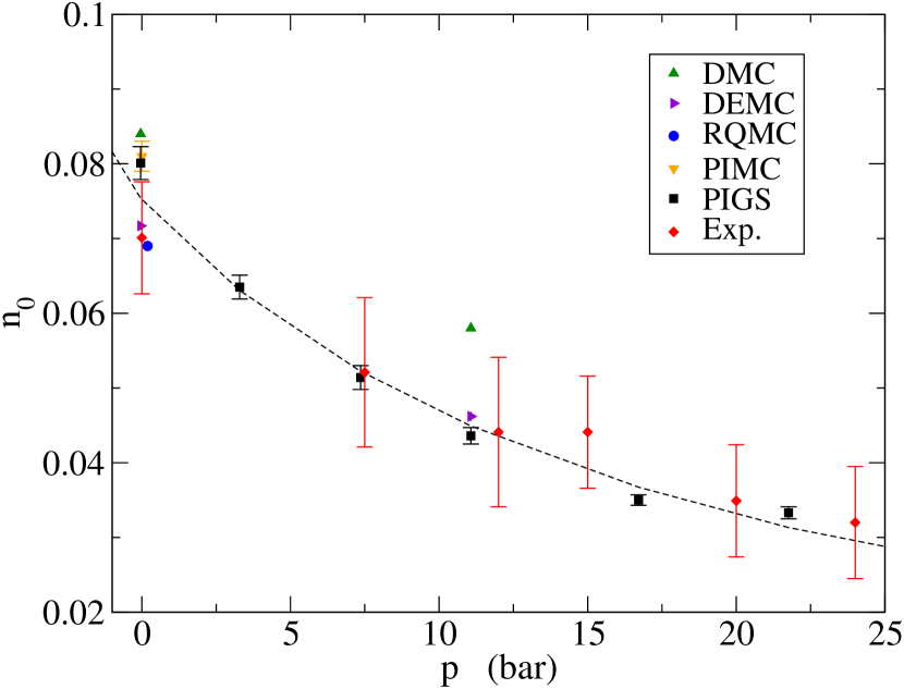
Figure 4: (Color online) The condensate fraction $n_{0}$ in liquid ⁴He at zero temperature as a function of pressure $p$ in the region of stability of liquid phase. Our PIGS results (black squares) are compared with the experimental ones (red diamonds) ⁶ and previous theoretical calculations, obtained with Diffusion Monte Carlo (green up triangles),¹⁰ Diffusion Euler Monte Carlo (violet left triangles),¹¹ Reptation Quantum Monte Carlo (blue circle) ¹³ and PIMC at $T=1\,{\rm K}$.⁹ The dashed line represents the curve obtained fitting our results with the equation $n_{0}=A+B/(p-p_{0})$.

IV Conclusions

We have computed the one-body density matrix of liquid ⁴He at zero temperature and different densities by means of the PIGS Monte Carlo method. Although it is not easy to give an analytic model to fit the data for $\rho_{1}(r)$, because of the difficulty of describing the coupling between the condensate and the excited states in strongly correlated quantum systems such as ⁴He, it is possible to extrapolate very precise estimates of the condensate fraction and of the kinetic energy of the system even from a simplified model for $\rho_{1}$. Our calculations provide an improvement with respect to the other ground state projection techniques used in the past, since the PIGS method allows us to remove completely the influence of any input trial wave function. Indeed, we have performed calculations of $\rho_{1}(r)$ and $n_{0}$ in liquid ⁴He at zero temperature using a model for the ground state wave function which depends uniquely on the Hamiltonian and on the symmetry properties of the system. At the equilibrium density of liquid ⁴He, we have recovered the value of $n_{0}$ obtained with the unbiased PIMC method at temperature $T=1\,{\rm K}$.⁹ Simulating the system at several densities, the dependence of $n_{0}$ with pressure $p$ obtained from the calculation agrees nicely with the recent experimental measurements of Ref. ⁶

Appendix A Appendix: full tables for the momentum distribution

The aim of this appendix is to provide the full table of the momentum distribution $n(k)$ in liquid ⁴He at zero temperature and different densities, obtained from Path Integral Ground State caluclations.

$\rho$ (Å-3)	0.01964	0.02186	0.02264	0.02341	0.02401	0.02479
k (Å-1)	n(k) (Å3)
0.4	0.10415	0.08758	0.08041	0.07708	0.07685	0.07078
0.5	0.09226	0.07838	0.07355	0.07082	0.06972	0.06509
0.6	0.08157	0.07009	0.06697	0.06448	0.06292	0.05937
0.7	0.07238	0.06298	0.06092	0.05833	0.05676	0.05390
0.8	0.06441	0.05687	0.05532	0.05244	0.05127	0.04877
0.9	0.05711	0.05130	0.04996	0.04682	0.04628	0.04397
1.0	0.04996	0.04581	0.04461	0.04141	0.04154	0.03941
1.1	0.04269	0.04011	0.03912	0.03619	0.03684	0.03499
1.2	0.03536	0.03417	0.03351	0.03116	0.03209	0.03066
1.3	0.02823	0.02818	0.02793	0.02637	0.02733	0.02644
1.4	0.02165	0.02244	0.02262	0.02186	0.02272	0.02238
1.5	0.01596	0.01727	0.01781	0.01771	0.01843	0.01858
1.6	0.01135	0.01291	0.01367	0.01401	0.01465	0.01514
1.7	0.00792	0.00948	0.01032	0.01082	0.01149	0.01215
1.8	0.00561	0.00699	0.00777	0.00824	0.00898	0.00965
1.9	0.00425	0.00533	0.00594	0.00630	0.00709	0.00767
2.0	0.00356	0.00433	0.00472	0.00495	0.00573	0.00617
2.1	0.00325	0.00374	0.00393	0.00408	0.00476	0.00506
2.2	0.00303	0.00334	0.00341	0.00354	0.00406	0.00424
2.3	0.00272	0.00296	0.00300	0.00314	0.00350	0.00361
2.4	0.00225	0.00252	0.00260	0.00276	0.00300	0.00308
2.5	0.00170	0.00201	0.00217	0.00232	0.00251	0.00258
2.6	0.00118	0.00149	0.00171	0.00184	0.00204	0.00210
2.7	0.00078	0.00106	0.00128	0.00138	0.00161	0.00166
2.8	0.00055	0.00077	0.00092	0.00100	0.00124	0.00127
2.9	0.00045	0.00061	0.00065	0.00074	0.00095	0.00097
3.0	0.00040	0.00053	0.00048	0.00058	0.00075	0.00076
3.1	0.00036	0.00048	0.00038	0.00049	0.00062	0.00062
3.2	0.00029	0.00042	0.00032	0.00041	0.00052	0.00053
3.3	0.00021	0.00027	0.00027	0.00032	0.00044	0.00046
3.4	0.00016	0.00021	0.00022	0.00023	0.00037	0.00039
3.5	0.00015	0.00017	0.00017	0.00015	0.00030	0.00031

Table 2: The momentum distribution $n(k)$ of liquid ⁴He at zero temperature as computed by Path Integral Ground State method for densities between $\rho=0.01964\,{\rm\AA}^{-3}$ and $\rho=0.02479\,{\rm\AA}^{-3}$

$\rho$ (Å-3)	0.02539	0.02623	0.02701	0.02785	0.02869	0.02940	0.02994
k (Å-1)	n(k) (Å3)
0.4	0.06464	0.06170	0.05811	0.05400	0.04904	0.04542	0.04310
0.5	0.06013	0.05751	0.05403	0.04993	0.04600	0.04291	0.04076
0.6	0.05554	0.05328	0.04990	0.04589	0.04286	0.04025	0.03828
0.7	0.05106	0.04916	0.04590	0.04210	0.03976	0.03753	0.03578
0.8	0.04673	0.04520	0.04211	0.03862	0.03677	0.03483	0.03330
0.9	0.04252	0.04134	0.03849	0.03541	0.03389	0.03217	0.03086
1.0	0.03834	0.03752	0.03499	0.03239	0.03107	0.02954	0.02843
1.1	0.03416	0.03367	0.03153	0.02942	0.02830	0.02694	0.02602
1.2	0.02995	0.02980	0.02807	0.02644	0.02552	0.02435	0.02359
1.3	0.02579	0.02594	0.02463	0.02343	0.02276	0.02178	0.02118
1.4	0.02177	0.02219	0.02127	0.02043	0.02003	0.01927	0.01879
1.5	0.01801	0.01864	0.01806	0.01751	0.01740	0.01684	0.01649
1.6	0.01462	0.01539	0.01510	0.01479	0.01491	0.01456	0.01430
1.7	0.01171	0.01253	0.01247	0.01234	0.01264	0.01245	0.01229
1.8	0.00931	0.01010	0.01021	0.01023	0.01063	0.01056	0.01048
1.9	0.00743	0.00814	0.00835	0.00848	0.00890	0.00892	0.00891
2.0	0.00602	0.00662	0.00687	0.00707	0.00746	0.00752	0.00756
2.1	0.00500	0.00549	0.00571	0.00595	0.00629	0.00636	0.00644
2.2	0.00425	0.00466	0.00481	0.00506	0.00533	0.00540	0.00550
2.3	0.00365	0.00402	0.00410	0.00433	0.00455	0.00461	0.00473
2.4	0.00312	0.00348	0.00350	0.00370	0.00388	0.00395	0.00407
2.5	0.00261	0.00296	0.00297	0.00314	0.00330	0.00337	0.00349
2.6	0.00211	0.00246	0.00248	0.00262	0.00278	0.00286	0.00297
2.7	0.00165	0.00198	0.00203	0.00215	0.00230	0.00240	0.00250
2.8	0.00126	0.00155	0.00162	0.00173	0.00188	0.00200	0.00208
2.9	0.00096	0.00121	0.00129	0.00139	0.00152	0.00164	0.00171
3.0	0.00076	0.00097	0.00102	0.00111	0.00122	0.00134	0.00140
3.1	0.00064	0.00081	0.00081	0.00090	0.00100	0.00111	0.00114
3.2	0.00055	0.00070	0.00066	0.00074	0.00082	0.00092	0.00094
3.3	0.00047	0.00061	0.00054	0.00062	0.00069	0.00077	0.00078
3.4	0.00039	0.00052	0.00044	0.00053	0.00058	0.00065	0.00066
3.5	0.00031	0.00043	0.00035	0.00044	0.00049	0.00055	0.00055

Table 3: The momentum distribution $n(k)$ of liquid ⁴He at zero temperature as computed by Path Integral Ground State method for densities between $\rho=0.02539\,{\rm\AA}^{-3}$ and $\rho=0.02994\,{\rm\AA}^{-3}$