Anisotropic vortex lattice structures in the FeSe superconductor

Abstract

In the recent work by Song et al. song2011 , the scanning tunneling spectroscopy experiment in the stoichiometric FeSe reveals evidence for nodal superconductivity and strong anisotropy. The nodal structure can be explained with the extended $s$-wave pairing structure with the mixture of the $s_{x^{2}+y^{2}}$ and $s_{x^{2}y^{2}}$ pairing symmetries. We calculate the anisotropic vortex structure by using the self-consistent Bogoliubov-de Gennes mean-field theory. In considering the absence of magnetic ordering in the FeSe at the ambient pressure, orbital ordering is introduced, which breaks the $C_{4}$ lattice symmetry down to $C_{2}$, to explain the anisotropy in the vortex tunneling spectra.

I Introduction

Since the first iron-based layered superconductor La(O_1-xF_x)FeAs had been discoveredkamihara2008 , the family of iron-based superconductors have brought huge impact in condensed matter physics community. These novel materials exhibit similar phase diagrams compared to high-T_c cuprates. The parent compound LaOFeAs has an antiferromagnetic spin-density-wave order lacruz2008 , and, upon doping, superconductivity appears. Although correlation effects are weaker in iron-based superconductors than those in high-T_c cuprates, novel features arise from the multi-orbital degree of freedom. The orbital band structures play fundamental roles in determining the Fermi surface configurations and pairing structures.

Understanding pairing symmetries is one of the most important issues in the study of iron-based superconductors. Based on various experimental hanaguri2010 ; ding2008 ; zhangxh2009 and theoretical works seo2008 ; daghofer2008 ; wang2008 ; tesanovic2009 ; tesanovic20092 , the nodeless $s_{x^{2}y^{2}}$-wave pairing has been proposed. In momentum space, the Fermi surfaces of many iron-based superconductors consist of hole pockets around the $\Gamma$-point, and electron pockets around the two $M$-points. The signs of the pairing order parameters on electron and hole Fermi surfaces are opposite. The nodal lines of the gap function have no intersections with Fermi surfaces, thus the $s_{x^{2}y^{2}}$-pairing is nodeless. In the itinerant picture, the Fermi surface nesting between the hole and the electron pockets facilitates the antiferromagnetic fluctuations which favor the $s_{x^{2}y^{2}}$-pairing norman2008 . In real space, an intuitive picture of the $s_{x^{2}y^{2}}$-wave pairing is just the next-nearest-neighbor (NNN) spin-singlet pairing with the $s$-wave symmetry seo2008 . Because the anion locations are above or below the centers of the iron-iron plaquettes, the NNN antiferromagnetic exchange $J_{2}$ is at the same order of the nearest neighbor (NN) one $J_{1}$. The NNN $s_{x^{2}y^{2}}$-wave pairing can be obtained from the decoupling of the $J_{2}$-term. On the other hand, various experimental results have shown signatures of nodal pairing structures fletcher2009 ; hicks2009 ; zeng2010 . In the framework of the $s$-wave pairing, the nodal pairing can be achieved through the $s_{x^{2}+y^{2}}$-pairing mazin2008 ; yao2009 ; wang2010 . The possibility for the $s_{x^{2}+y^{2}}$-wave pairing in iron-based superconductors has also been shown in the functional renormalization-group calculation wang2009 .

Another important aspect of the iron-based superconductors is the spontaneous anisotropy of both the lattice and electronic degrees of freedom, which reduces the 4-fold rotational symmetry to 2-fold. For example, LaOFeAs undergoes a structural orthorhombic distortion and a long-range spin-density wave (SDW) order at the wavevector $(\pi,0)$ or $(0,\pi)$ lacruz2008 . Similar phenomenon was also detected in NdFeAsO by using polarized and unpolarized neutron-diffraction measurements chen2008 . One popular explanation of the nematicity is the coupling between lattice and the stripe-like SDW order fang2008 ; xu2008 . The SDW ordering has also been observed in the FeTe system but with a different ordering wavevector at $(\frac{\pi}{2},\frac{\pi}{2})$ li2009 ; bao2009 .

Very recently, the experimental results of the FeSe superconductor reported by Song et al.song2011 indicate a pronounced nodal pairing structure in the scanning-tunneling-spectroscopy. Strong electronic anisotropy is observed through the quasi-particle interference of the tunneling spectra at much higher energy than the superconducting gap. The low energy tunneling spectra around the impurity and the vortex core also exhibit the anisotropy. The shapes of the vortex cores are significantly distorted along one lattice axis.

The anisotropy may arise from the structural transition from tetragonal to orthorhombic phase at $90$K. However, the typical orthorhombic lattice distortions in iron superconductors are at the order of $0.012\AA$, which is about half a percent of the lattice constant and only lead to a tiny anisotropy in electronic structuressong2011 . In contrast, the anisotropic vortex cores and impurity tunneling spectra observed by Song et al. are clearly at the order of one. Therefore these anisotropies should be mainly attributed to the electronic origin. The antiferromagnetic long-range-order in such a system may be a possible reason for the anisotropy. For example, it has been theoretically investigated that the stripe-like SDW order can induce strong anisotropy in the quasi-particle interference of the STM tunnelling spectroscopy knolle2010 . However, no evidence of magnetic ordering has been found in FeSe at ambient pressure medvedev2009 , thus this anisotropy should not be directly related to the long-range magnetic ordering.

On the other hand, orbital ordering is another possibility for nematicity in transition metal oxides. For example, orbital ordering serves as a possible mechanism for the nematic metamagnetic states observed in Sr₃Ru₂O₇ leewc2009 ; raghu2009 , and its detection through quasi-particle interference has been investigated leewc2010 ; leewc2009a . Orbital ordering has also been suggested to lift the degeneracy between the $d_{xz}$ and $d_{yz}$-orbitals to explain the anisotropy in iron-based superconductors.

In this article, we will study the effect of orbital ordering to the vortex tunneling spectra in the FeSe superconductor. The rest of the paper is organized as follows. In Sec. II, a two-band model Hamiltonian and the relevant band parameters are introduced. The Bogoliubov-de Gennes mean-filed formalism is described in Sec. III. In Sec. IV, we analyze the effects of orbital ordering to the tunneling spectra of mixed pairing of the NN $s_{x^{2}+y^{2}}$-wave and the NNN $s_{x^{2}y^{2}}$-wave in the homogeneous systems. In Sec. V, the effects of orbital ordering to the anisotropic vortex core tunneling spectra are investigated, which are in a good agreement with experiments. Discussions and conclusions are given in Sec. VI.

II Model Hamiltonian for the band structure

For simplicity, we use the two-band model involving the $d_{xz}$ and $d_{yz}$-orbital bands in a square lattice with each lattice site representing an iron atom, which was first proposed in Ref. [raghu2008, ]. This is the minimal model describing the iron-based superconductors, which can also support orbital ordering. The tight-binding band Hamiltonian reads

$$H_{0} = \sum_{\vec{r},\sigma}\Big{\{}H^{nn}_{\parallel,\sigma}+H^{nn}_{\perp,\sigma}+H^{nnn}_{\sigma}-\mu n_{\vec{r}}\Big{\}},$$ (1)

where

$$H^{nn}_{\parallel,\sigma} = t^{nn}_{\parallel}(d^{{\dagger}}_{xz,\sigma,\vec{r}}d_{xz,\sigma,\vec{r}+\hat{x}}+d^{{\dagger}}_{yz,\sigma,\vec{r}}d_{yz,\sigma,\vec{r}+\hat{y}}),$$

$$H^{nn}_{\perp,\sigma} = t^{nn}_{\perp}(d^{{\dagger}}_{xz,\sigma,\vec{r}}d_{xz,\sigma,\vec{r}+\hat{y}}+d^{{\dagger}}_{yz,\sigma,\vec{r}}d_{yz,\sigma,\vec{r}+\hat{x}}),$$

$$H^{nnn}_{\sigma} = t^{nnn}_{1}(d^{{\dagger}}_{xz,\sigma,\vec{r}}d_{xz,\sigma,\vec{r}\pm\hat{x}+\hat{y}}+d^{{\dagger}}_{yz,\sigma,\vec{r}}d_{yz,\sigma,\vec{r}\pm\hat{x}+\hat{y}})$$

$$+ t^{nnn}_{2}(d^{{\dagger}}_{xz,\sigma,\vec{r}}d_{yz,\sigma,\vec{r}+\hat{x}+\hat{y}}+d^{{\dagger}}_{yz,\sigma,\vec{r}}d_{xz,\sigma,\vec{r}+\hat{x}+\hat{y}})$$

$$+ t^{nnn}_{3}(d^{{\dagger}}_{xz,\sigma,\vec{r}}d_{yz,\sigma,\vec{r}-\hat{x}+\hat{y}}+d^{{\dagger}}_{yz,\sigma,\vec{r}}d_{xz,\sigma,\vec{r}-\hat{x}+\hat{y}}),$$

where $d^{{\dagger}}_{a,\sigma,\vec{r}}$ denotes the creation operator for an electron with spin $\sigma$ on $d_{a}$-orbital at site $\vec{r}$; $d_{a}$ refers to $d_{xz}$ and $d_{yz}$-orbitals; $n_{\vec{r}}=n_{xz,\sigma,\vec{r}}+n_{yz,\sigma,\vec{r}}$ where $n_{a,\sigma,\vec{r}}=d^{{\dagger}}_{a,\sigma,\vec{r}}d_{a,\sigma,\vec{r}}$ denotes the particle number operator; $\mu$ is the chemical potential; $t^{nn}_{\parallel}$ and $t^{nn}_{\perp}$ denote the longitudinal $\sigma$-bonding and transverse $\pi$-bonding between nearest-neighboring (NN) sites, respectively; the three next-nearest-neighboring (NNN) hoppings can be expressed in terms of the NNN $\sigma$ and $\pi$-bondings $t^{nnn}_{\parallel}$ and $t^{nnn}_{\perp}$, respectively as $t^{nnn}_{1}=\frac{1}{2}(t^{nnn}_{\parallel}+t^{nnn}_{\perp})$, $t^{nnn}_{2}=\frac{1}{2}(t^{nnn}_{\parallel}-t^{nnn}_{\perp})$, and $t^{nnn}_{3}=\frac{1}{2}(-t^{nnn}_{\parallel}+t^{nnn}_{\perp})$. We depict the hopping schematic of the two-band tight-binding model Eq. (1) in Fig. 1.

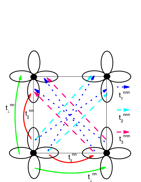
Figure 1: (Color online) The hopping schematic of the two-band tight-binding model Eq. (1) in a unit cell. Each black solid circle represents an Fe atom. The solid arrows denote NN longitudinal $\sigma$-bonding (red) and transverse $\pi$-bonding (green) hoppings, respectively. The NNN intra-orbital hoppings $t^{nnn}_{1}$ are indicated by blue dot arrows along $\pm\hat{x}+\hat{y}$ directions. On the other hand, the NNN inter-orbital hoppings, $t^{nnn}_{2}$ and $t^{nnn}_{3}$, along the $\hat{x}+\hat{y}$ and $-\hat{x}+\hat{y}$ directions, respectively, are indicated by dash arrows labeled with cyan and pink.

By introducing the spinor $\Psi(\vec{k})=[\psi_{xz,\sigma}(\vec{k}),\psi_{yz,\sigma}(\vec{k})]^{T}$ and performing the Fourier transformation, the Hamiltonian in momentum space becomes

$$H_{0}=\sum_{\vec{k}}\Psi^{{\dagger}}_{a,\sigma}(\vec{k})\Big{\{}H_{ab}(\vec{k})+\varepsilon(\vec{k})-\mu\delta_{ab}\Big{\}}\Psi_{b,\sigma}(\vec{k}),$$ (3)

where $a,b$ refer to the band index; the matrix kernel $H_{ab}(\vec{k})$ is written as

$$\left(\begin{array}[]{cc}2t^{nn}_{\parallel}\cos{k_{x}}+2t^{nn}_{\perp}\cos{k_{y}}&4t^{nnn}_{3}\sin{k_{x}}\sin{k_{y}}\\ h.c.&2t^{nn}_{\parallel}\cos{k_{y}}+2t^{nn}_{\perp}\cos{k_{x}}\end{array}\right),$$ (6)

and $\varepsilon(\vec{k})=2\cos{k_{x}}\cos{k_{y}}(t^{nnn}_{\parallel}+t^{nnn}_{\perp})$. This two-orbital model has also been used to study impurity resonance states tsai2009 ; zhou2009 , vortex core states hu2009 ; jiang2009 , and quasiparticle scattering inference zhang2009 .

To fit the Fermi surface obtained from the LDA calculations xu2008 , we use the parameter values below in the following discussions as

$$t^{nn}_{\parallel}=0.8,~{}t^{nn}_{\perp}=-1.4,~{}t^{nnn}_{\perp}=1.8,~{}t^{nnn}_{\parallel}=0,$$ (7)

all which are in units of $t=1$, which is roughly at the energy scale around $100$meV. This set of hopping integrals shows a similar band structure, as the one Raghu et al. used. The band-width is about $14$. In the following discussion, we use $\mu=1.15$ which corresponds to slightly hole doped regimes. The unfolded Brillouin zone (UBZ) embraces a hole surface around the $\Gamma$ point [$\vec{k}=(0,0)$], and four hole pockets around the $X$ point [$\vec{k}=(\pm\pi,\pm\pi)$] and four electron pockets around $M$ point [$\vec{k}=(0,\pm\pi)$ or $(\pm\pi,0)$] norman2008 ; lebegue2007 .

Our main purpose is to study the anisotropy effects in FeSe due to the orbital ordering. Orbital ordering has been proposed in iron-based superconductors in previous studies kruger2009 ; lee2009 ; lv2009 ; chen2010 ; lv2010 ; lv2011 . Such an ordering may arise from the interplay between orbital, lattice, and magnetic degrees of freedom in iron superconductors. In this article, we are not interested in the microscopic mechanism of spontaneous orbital ordering, but rather assume its existence to explain the vortex tunneling spectra observed in Ref. [song2011, ]. According to the experimental data song2011 , strong anisotropy has already been observed at least at the energy scale of 10meV, which is much larger than the pairing gap value around 2meV. Thus when studying superconductivity, we neglect the fluctuations of the orbital ordering, but treat it as an external anisotropy. For this purpose, we add an extra anisotropy term into the band structure Eq. (1) as

$$H_{orb}=\delta\varepsilon\sum_{\vec{r},\sigma}(d^{{\dagger}}_{xz,\sigma,\vec{r}}d_{xz,\sigma,\vec{r}}-d^{{\dagger}}_{yz,\sigma,\vec{r}}d_{yz,\sigma,\vec{r}}),$$ (8)

which makes the $d_{xz}$-orbital energy higher than that of $d_{yz}$. For comparison, the Fermi surfaces without and with the anisotropy term Eq. (8) are depicted in Fig. 2 (a) and (b), respectively. In Fig. 2 (b), with the orbital term, the distortion of the electron and hole pockets in $x$ and $y$-directions of the Fermi surfaces appears such that the anisotropy is derived in the iron-based superconductors.

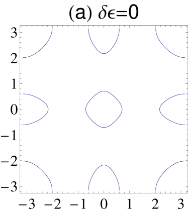
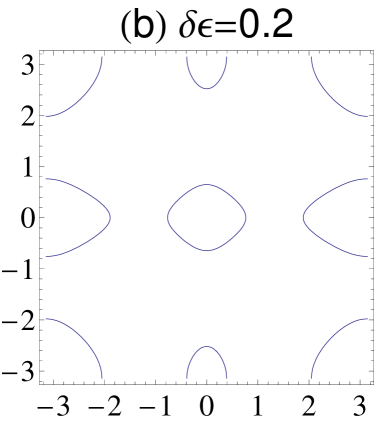
Figure 2: Fermi surfaces in the UBZ for (a) $\delta\varepsilon=0$ and (b) $\delta\varepsilon=0.2$. The horizontal and vertical axes denote $k_{x}$ and $k_{y}$, respectively. The parameter values used are $t^{nn}_{\parallel}=0.8$, $t^{nn}_{\perp}=-1.4$, $t^{nnn}_{\perp}=1.8$, $t^{nnn}_{\parallel}=0$, and $\mu=1.15$. Anisotropic hole and electron pockets are shown in (b) at the $\Gamma$ and $M$-points, respectively.

III The Bogoliubov-de Gennes formalism

In this section, we present the self-consistent Bogoliubov-de Gennes (BdG) formalism based on the band structure described in Sec. II. In principle, for this multi-orbital system, the general pairing structure should contain a matrix structure involving both the intra and inter-orbital pairings. Here for simplicity, we only keep the intra-orbital pairing which is sufficient to describe the anisotropy observed in the experiment by Song et al. song2011 .

The pairing interactions including the NN and NNN pairing are defined as

$$H_{int} = -\frac{g_{1}}{2}\sum_{\langle\vec{r},\vec{r}^{\prime}\rangle}\sum_{a}\hat{\Delta}^{{\dagger}}_{a}(\vec{r},\vec{r}^{\prime})\hat{\Delta}_{a}(\vec{r},\vec{r}^{\prime}),$$ (9)

$$- \frac{g_{2}}{2}\sum_{\langle\langle\vec{r},\vec{r}^{\prime}\rangle\rangle}\sum_{a}\hat{\Delta}^{{\dagger}}_{a}(\vec{r},\vec{r}^{\prime})\hat{\Delta}_{a}(\vec{r},\vec{r}^{\prime}),$$

where $a$ is the orbital index taking values of $d_{xz}$ and $d_{yz}$; $\langle\vec{r},\vec{r}^{\prime}\rangle$ represents the NN-bonds and $\langle\langle\vec{r},\vec{r}^{\prime}\rangle\rangle$ represents the NNN-bonds; $g_{1,2}$ denotes the pairing interaction strengths along the NN and NNN-bonds; $\hat{\Delta}_{a}(\vec{r},\vec{r}^{\prime})$ describes the spin singlet intra-orbital pairing operator across the bond defined as

$$\hat{\Delta}_{a}(\vec{r},\vec{r}^{\prime})=d_{a,\downarrow,\vec{r}}d_{a,\uparrow,\vec{r}^{\prime}}-d_{a,\uparrow,\vec{r}}d_{a,\downarrow,\vec{r}^{\prime}}.$$ (10)

where $\vec{r}^{\prime}=\vec{r}+\vec{\delta}$. For the $s_{x^{2}+y^{2}}$-pairing along the NN-bonds, $\vec{\delta}=a\hat{x}(\hat{y})$, whereas for the $s_{x^{2}y^{2}}$-pairing along the NNN-bonds, $\vec{\delta}=\pm a(\hat{x}+\hat{y})$ NNN-bonds, where $a$ is Fe-Fe bond length, defined as the lattice constant. In the square lattice, these two pairings belong to the same symmetry class, thus they naturally coexist. After the mean-field decomposition, the Hamiltonian becomes

$$H_{MF} = H_{0}-\frac{g_{1}}{2}\sum_{\langle\vec{r},\vec{r}^{\prime}\rangle}\sum_{a}\Delta^{*}_{a}(\vec{r},\vec{r}^{\prime})\hat{\Delta}_{a}(\vec{r},\vec{r}^{\prime})$$ (11)

$$- \frac{g_{2}}{2}\sum_{\langle\langle\vec{r},\vec{r}^{\prime}\rangle\rangle}\sum_{a}\Delta^{*}_{a}(\vec{r},\vec{r}^{\prime})\hat{\Delta}_{a}(\vec{r},\vec{r}^{\prime})+h.c.,$$

where $\Delta^{*}_{a}(\vec{r},\vec{r}^{\prime})=\langle\hat{\Delta}^{{\dagger}}_{a}(\vec{r},\vec{r}^{\prime})\rangle$ is the pairing order parameter and $\langle\cdots\rangle$ denotes the expectation value over the ground state.

The mean-field BdG Hamiltonian Eq. (11) can be diagonalized through the transformation as

$${c_{a,\uparrow}(\vec{r})\choose c^{{\dagger}}_{a,\downarrow}(\vec{r})}=\sum_{n}\left(\begin{array}[]{cc}u_{a,n}(\vec{r})&-v^{*}_{a,n}(\vec{r})\\ v_{a,n}(\vec{r})&u^{*}_{a,n}(\vec{r})\end{array}\right){\gamma_{a,n}\choose\gamma^{{\dagger}}_{a,n}}.$$ (14)

The eigenvectors associated with $E_{n}$ of the above BdG equations are $(u_{a,n}(\vec{r}),v_{a,n}(\vec{r}))^{T}$ and the pairing order parameters can be further obtained self-consistently as

$$\Delta_{a}(\vec{r},\vec{r}^{\prime})=\sum_{n}(u_{n}(\vec{r})v^{*}_{n}(\vec{r}^{\prime})+u_{n}(\vec{r}^{\prime})v^{*}_{n}(\vec{r}))\tanh{\frac{bE_{n}}{2}},$$

where $b=1/k_{B}T$. After the wave functions are obtained self-consistently, the local density of states (LDOS), which is proportional to the conductance ($dI/dV$) in the scanning tunneling microscopy, can be further measured by

$$\rho(\vec{r},E) = \sum_{n,a}\Big{\{}|u_{a,n}(\vec{r})|^{2}L(E-E_{n})$$ (16)

$$+ |v_{a,n}(\vec{r})|^{2}L(E+E_{n})\Big{\}},$$

where $L(x)$ is the Lorentzian as $L(x)=\gamma/[\pi(x^{2}+\gamma^{2})]$ and $\gamma$ means the energy-broadening parameters, usually set around $10^{-2}$.

When we study the vortex lattice structure problem, the single particle Hamiltonian Eq. (1) is modified by the magnetic vector potential as

$$H_{0}^{\prime}=\sum_{\vec{r}_{i},\vec{r}_{j},\sigma,a,b}t_{i,j;a,b}e^{i\frac{\pi}{\Phi_{0}}\int^{\vec{r}_{i}}_{\vec{r}_{j}}\vec{A}(\vec{r})\cdot d\vec{r}}d^{{\dagger}}_{a,\sigma,\vec{r}_{i}}d_{b,\sigma,\vec{r}_{j}},$$ (17)

where $\Phi_{0}=hc/2e$ is the quantized flux; $a,b$ denote orbital indices and $\sigma$ denotes the spin index; $t_{i,j;a,b}$ represents $t^{nn}_{\parallel}$, $t^{nn}_{\perp}$ or $t^{nnn}_{1,2,3}$ depending on the corresponding bonds and orbitals. The vector potential $\vec{A}(\vec{r})$ is chosen as the Landau gauge by $(A_{x},A_{y})=(0,Bx)$.

Due to the magnetic translational symmetry, we can apply the magnetic periodic boundary conditions to form Abrikosov vortex lattices. Each magnetic unit cell carries a magnetic flux of $2\Phi_{0}$, so that each magnetic unit cell contains two vortices. We choose the size of the magnetic unit cell $pa\times qa$ with $p=2q$, and the number of unit cells $N_{x}\times N_{y}$ with $N_{y}=2N_{x}$. The corresponding magnetic field is $B=2\Phi_{0}/pqa^{2}=\Phi_{0}/(qa)^{2}$. In the Abrikosov vortex lattice, the translation vector is written as $\vec{\textrm{V}}=(\textrm{X}pa,\textrm{Y}qa)$, where $\textrm{X}=0,\cdots,N_{x}-1$ and $\textrm{Y}=0,\cdots,N_{y}-1$ are integers. The coordinate of an arbitrary lattice site can be expressed as $\vec{R}=\vec{r}+\vec{\textrm{V}}$, where $\vec{r}=(xa,ya)$ denotes the coordinate of the lattice site within a magnetic unit cell, i.e. $1\leq x\leq p$ and $1\leq y\leq q$.

Under the magnetic periodic boundary conditions, the eigenvectors of the BdG equations Eq. (14) satisfy a periodic structure written as

$$\left(\begin{array}[]{c}u_{a,n}(\vec{r}+pa\hat{x})\\ v_{a,n}(\vec{r}+pa\hat{x})\end{array}\right) = e^{iK_{x}}\left(\begin{array}[]{c}e^{2\pi i\frac{y}{q}}u_{a,n}(\vec{r})\\ e^{-2\pi i\frac{y}{q}}v_{a,n}(\vec{r})\end{array}\right),$$ (22)

$$\left(\begin{array}[]{c}u_{a,n}(\vec{r}+qa\hat{y})\\ v_{a,n}(\vec{r}+qa\hat{y})\end{array}\right) = e^{iK_{y}}\left(\begin{array}[]{c}u_{a,n}(\vec{r})\\ v_{a,n}(\vec{r})\end{array}\right).$$ (27)

Here $K_{x}=\frac{2\pi\textrm{X}}{N_{x}}$ and $K_{y}=\frac{2\pi\textrm{Y}}{N_{y}}$ represent the magnetic Bloch wavevector on the x and y componentshan2010 . With the relation, we can simulate vortex lattices with sizes of $(N_{x}pa)\times(N_{y}qa)$ but reduce the computational effort by diagonalizing $N_{x}N_{y}$ Hamiltonian matrices with dimensions of $4pq$ rather than directly diagonalizing a $4N_{x}N_{y}pq$ Hamiltonian matrix.

IV The nodal v.s. nodeless pairings

In this section, we investigate the behavior of the superconducting gaps in the homogeneous system. Due to the translation symmetry, the pairing order parameters are spatially uniform, and we define $\Delta_{a}(\vec{\delta})=\Delta_{a}(\vec{r},\vec{r}+\vec{\delta})$ where $a=d_{xz},d_{yz}$. We start with the case in the absence of orbital ordering, i.e., $\delta\varepsilon=0$. Due to the four-fold rotational symmetry, not all of the pairing order parameters are independent. For the NN bond pairing, we have $\Delta_{xz}(\hat{x})=\Delta_{yz}(\hat{y})$ and $\Delta_{xz}(\hat{y})=\Delta_{yz}(\hat{x})$ due to the $s$-wave symmetry. As for the NNN-bonding, the similar analysis yields the following relations of $\Delta_{xz}(\hat{x}+\hat{y})=\Delta_{yz}(-\hat{x}+\hat{y})$, and $\Delta_{xz}(\hat{x}-\hat{y})=\Delta_{yz}(\hat{x}+\hat{y})$.

Due to the multi-orbital structure, generally speaking, the pairing order parameters have the matrix structure, thus the analysis of the pairing symmetry is slightly complicated. However, before the detailed calculation, we perform a simplified qualitative analysis by considering the trace of the pairing matrix, defined as

$$\Delta(\vec{\delta})=\frac{1}{2}\big{(}\Delta_{xz}(\vec{\delta})+\Delta_{yz}(\vec{\delta})\big{)}$$ (28)

for both of the NN and NNN-bonds. These quantities play the major role in determining the pairing symmetry. The angular form factor of the Fourier transform of the NN $s$-wave pairing is $\Delta_{s_{x^{2}+y^{2}}}(k_{x},k_{y})\propto\cos{k_{x}}+\cos{k_{y}}$, and that of the NNN $s$-wave is $\Delta_{s_{x^{2}y^{2}}}(k_{x},k_{y})\propto\cos{k_{x}}\cos{k_{y}}$. Naturally $\Delta_{s_{x^{2}+y^{2}}}$ and $\Delta_{x^{2}y^{2}}$ have the same phase. Otherwise there would be a large energy cost corresponding to the phase twist in a small length scale of lattice constant. The nodal lines of $\Delta_{s_{x^{2}+y^{2}}}$ have intersections with the electron pockets, while the nodal lines of $\Delta_{x^{2}y^{2}}$ have not intersections with Fermi surfaces. Generally speaking, the NN and NNN $s$-wave pairings are mixed due to the same symmetry representation to the lattice group as

$$\Delta_{s_{\pm}}(k_{x},k_{y})=\Delta_{1}(\cos{k_{x}}+\cos{k_{y}})+\Delta_{2}\cos{k_{x}}\cos{k_{y}}.$$

(29)

It is well-known that the gap function is nodal for the NN $s$-wave pairing; while it is nodeless for the NNN $s$-wave pairing. However, they can mix together. Recently this aspect was supported by a variational Monte-Carlo calculation,yang2010 where the authors discovered that the $s_{x^{2}y^{2}}$-wave and $s_{x^{2}+y^{2}}$-wave states are energetically comparable. Our BdG calculations show that even for the case of $g_{2}\neq 0$ and $g_{1}=0$, the $s$-wave NN pairing is still induced by the $g_{2}$ term, and vice versa for the $s$-wave NNN pairing showing that they can naturally coexist.

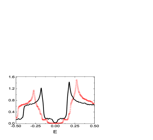
Figure 3: DOS v.s. tunneling bias $E$ for the mixed $s$-wave pairing states at the zero temperature. The red hollow squares with the parameter depict the nodeless pairing with the dominant NNN pairing; and the black solid line depicts the nodal pairing with the dominant NN pairing. The parameter values are $(g_{1}=0.8,g_{2}=1.2)$ for the nodeless case and $(g_{1}=1.2,g_{2}=0.4)$ for the nodal case, respectively.

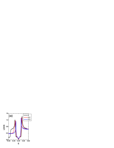
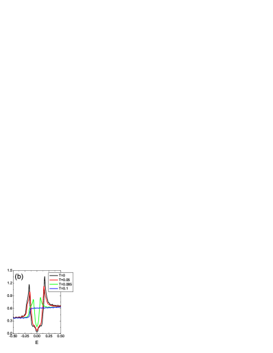
Figure 4: (a) DOS v.s. tunneling voltage $E$ for extended $s_{\pm}$-wave without orbital anisotropy ($\delta\varepsilon=0$), and the orbital anisotropy $(\delta\varepsilon=0.2,0.3)$. Other parameter values are $(g_{1}=1.2,g_{2}=0.4)$. At $\delta\varepsilon=0$ the coherent peaks are around $E=\pm 0.18$ and upon increasing $\delta\varepsilon=0$ the locations of the coherent peaks only slightly move towards zero energy. (b) The temperature dependence of the DOS v.s. $E$ for the extended $s_{\pm}$-wave with orbital anisotropy $\delta\varepsilon=0.2$ and the same parameters of $g_{1,2}$ as in (a). At $T=0$, the coherent peaks are located at $E=\pm 0.165$.

For the coexistence of the NN and NNN $s$-wave pairing, the pairing gap function can be either nodal or nodeless. For the pure NNN $s$-wave pairing, the nodal lines of the $\Delta_{x^{2}y^{2}}$ are $k_{x,y}=\pm\frac{\pi}{2}$, which have no intersections with all of the hole and electron pockets, thus the pairing is nodeless. For the pure NN $s$-wave pairing, the nodal lines form a diamond box with four vertices at the M-points $(\pm\pi,0)$ and $(0,\pm\pi)$, which intersects both electron pockets, thus the pairing is nodal. When the NN and NNN $s$-wave pairings coexist, if the NN $s_{x^{2}+y^{2}}$-wave pairing is dominant, the nodal lines of the pairing function is illustrated in the Fig. S6 (a) of Ref. [song-supp, ]. The original diamond nodal box is deformed by pushing the four vertices way from the $M$-points to the direction of the $\Gamma$-point. If the deformation is small, the deformed diamond still intersects with the electron pockets, and thus the pairing remains nodal. Upon increasing the strength of the NNN pairing, the deformation is enlarged and the intersections disappear. Thus the pairing is nodeless.

Fig. 3 reveals the density of states (DOS) v.s. tunneling voltage for the mixed $s$-wave pairing state. The red hollow squares are obtained using stronger NNN pairing strength [i.e. $g_{1}=0.8$ and $g_{2}=1.2$ in Eq. (11)], providing gapful behavior which is similar to the pure $s_{x^{2}y^{2}}$-wave state. In this case, $\Delta_{xz}(\hat{x})=\Delta_{yz}(\hat{y})=0.068$, $\Delta_{xz}(\hat{y})=\Delta_{yz}(\hat{x})=-0.077$ and $\Delta_{xz,yz}(\pm\hat{x}\pm\hat{y})=0.085$ showing stronger NNN $s_{x^{2}y^{2}}$-wave pairing than NN $s_{x^{2}+y^{2}}$-wave pairing. On the other hand, the black solid line (using $g_{1}=1.2$ and $g_{2}=0.4$) indicates a gapless $V$-shape, similar to the pure $s_{x^{2}+y^{2}}$-wave state. In contrary to the former case, the NN pairing order parameters $\Delta_{xz}(\hat{x})=\Delta_{yz}(\hat{y})=0.071$, $\Delta_{xz}(\hat{y})=\Delta_{yz}(\hat{x})=-0.059$ are larger than NNN $s_{x^{2}y^{2}}$-wave ones $\Delta_{xz,yz}(\pm\hat{x}\pm\hat{y})=0.057$. This reveals that the competition between the gapful and gapless modes can be adjusted by tuning the ratios between NNN and NN pairing interactions.

The main goal of our paper is the effect from orbital ordering which is mimicked by Eq. (8). With the anisotropy, the pairing structure changes from Eq. (29) to the following

$$\Delta_{s_{\pm}}(k_{x},k_{y}) = \Delta_{1}(\cos{k_{x}}+\lambda\cos{k_{y}})$$ (30)

$$+ \Delta_{2}\cos{k_{x}}\cos{k_{y}},$$

where $\lambda$ is determined by the anisotropy. The anisotropic nodal curve still intersects the electron pockets as illustrated in the Fig. S6 (b) in Ref. song-supp, , and thus the superconducting gap functions remain nodal. The calculated DOS vs energy patterns are plotted in Fig. 4 (a) with the parameter values specified in the figure caption. Upon finite $\delta\varepsilon$, the pairing order parameters become anisotropic. For example, at $\delta\varepsilon=0.2$, we have

$$\Delta_{xz}(\hat{x})=0.059,\ \ \,\ \ \,\Delta_{yz}(\hat{y})=0.070,$$

$$\Delta_{xz}(\hat{y})=-0.050,\ \ \,\Delta_{yz}(\hat{x})=-0.054,$$

$$\Delta_{xz}(\hat{x}+\hat{y})=\Delta_{xz}(-\hat{x}+\hat{y})=0.0503$$

$$\Delta_{yz}(\hat{x}+\hat{y})=\Delta_{yz}(-\hat{x}+\hat{y})=0.0505,$$ (31)

and the gapless gap function and the $V$-shaped spectra remain in the moderate anisotropy from orbital ordering.

We also check the temperature dependence of DOS with the orbital ordering as presented in Fig. 4 (b) with same parameter values of $g_{1,2}$ as in Fig. 4 (a). With orbital anisotropy $\delta\varepsilon=0.2$, the coherence peaks at zero temperature is approximately $\Delta_{ch}\approx 0.165$. At low finite temperatures, say $T=0.05\approx 0.3\Delta_{ch}$, the $V$-shape DOS is still discernible. However, upon increasing temperatures the $V$-shaped LDOS patterns smear and eventually the coherent peaks disappear at $T=0.1\approx 0.6\Delta_{ch}$. In this case the system turns into the normal state. This feature is qualitatively consistent with the experimental observation of the differential conductance spectra on FeSe in Ref. [song2011, ].

V The vortex structure

In this section, we will study the vortex tunneling spectra for the extended $s_{\pm}$-wave state. The size of the magnetic unit cell is chosen as $pa\times qa=20a\times 40a$, which contains two vortices. The external magnetic field $B=2\Phi_{0}/pqa^{2}$. The number of magnetic unit-cells shown below is using $N_{x}\times N_{y}=20\times 10$, which is equivalent to the system size of $400a\times 400a$. The BdG equations are solved self-consistently with the tight-binding model Eq. (17) plus the mean-field interaction Eq. (9). The vortex configurations are investigated for both cases with and without orbital ordering in Sec. V.1 and Sec. V.2, respectively. The interaction parameters are $g_{1}=1.2$ and $g_{2}=0.4$, and the temperature is fixed at zero.

V.1 Vortex structure in the absence of orbital ordering

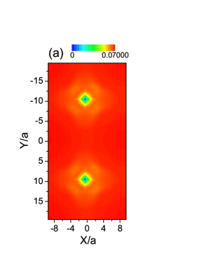
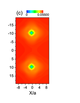
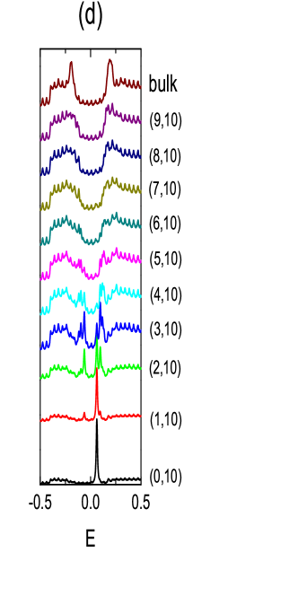
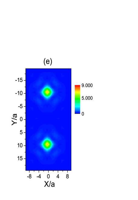
Figure 5: The vortex structure for the mixed NN $s_{x^{2}+y^{2}}$-wave NNN $s_{x^{2}y^{2}}$-wave pairing without orbital ordering. (a) and (b) depict the spatial distribution of the longitudinal and transverse NN pairings $\Delta^{NN}_{L}(\vec{r})$ and $\Delta^{NN}_{T}(\vec{r})$, respectively. (c) describes the NNN $s$-wave pairing order parameters $\Delta^{NNN}(\vec{r})$. (d) The LDOS v.s. E at different locations from the vortex core [at $\vec{r}=(0,10a)$] to outside along the $x$-axis. The distances of each site from the vortex core take the step of one lattice constant. (e) The spatial LDOS distribution at the energy of the vortex core resonance peak $E_{re}\approx 0.062$.

We start with the vortex configuration without orbital ordering. The NN $s_{x^{2}+y^{2}}$-wave and NNN $s_{x^{2}y^{2}}$-wave pairing order parameters in real space as defined as follows. We define the longitudinal and transverse NN $s$-wave pairings as

$$\Delta^{NN}_{L}(\vec{r}) = \frac{1}{4}\Big{\{}\Delta_{xz}(\vec{r},\vec{r}+a\hat{x})+\Delta_{xz}(\vec{r},\vec{r}-a\hat{x})$$

$$+ \Delta_{yz}(\vec{r},\vec{r}+a\hat{y})+\Delta_{yz}(\vec{r},\vec{r}-a\hat{y})\Big{\}}$$

$$\Delta^{NN}_{T}(\vec{r}) = \frac{1}{4}\Big{\{}\Delta_{yz}(\vec{r},\vec{r}+a\hat{x})+\Delta_{yz}(\vec{r},\vec{r}-a\hat{x})$$ (32)

$$+ \Delta_{xz}(\vec{r},\vec{r}+a\hat{y})+\Delta_{xz}(\vec{r},\vec{r}-a\hat{y})\Big{\}}.$$

For the NNN pairing related to site $\vec{r}$, we define

$$\Delta^{NNN}(\vec{r})=\frac{1}{8}\sum_{a=xz,yz;\vec{\delta}=\pm\hat{x}\pm\hat{y}}\Delta_{a}(\vec{r},\vec{r}+\vec{\delta}).$$ (33)

The pure NN $s_{x^{2}+y^{2}}$-wave vortex states are recently investigated to describe the competition between the superconductivity and spin-density-wave (SDW) in the hole-doped materials, Ba_1-xK_xFe₂As₂ gao2010 . Similar calculation for the pure NNN $s_{x^{2}y^{2}}$-wave with SDW has been used to study BaFe_1-xCo_xAs₂ hu2009 and the FeAs stoichiometric compoundsjiang2009 . In our case, these two $s$-wave pairing order parameters mix together.

The real space profiles of the longitudinal and transverse NN $s$-wave pairings $\Delta^{NN}_{L}(\vec{r})$ and $\Delta^{NN}_{T}(\vec{r})$ are depicted in Fig. 5 (a) and (b), respectively. The vortex cores are located at $\vec{r}=(0,\pm 10a)$ where the pairing order parameters are suppressed. Both of them exhibit the $C_{4}$ symmetry. The NNN $s$-wave pairing order parameters are depicted in Fig. 5 (c) and the vortices are diamond-shaped with the $C_{4}$ rotational symmetry. Note that the maximum magnitudes of the NNN $s_{x^{2}y^{2}}$-wave pairing order parameters are smaller than those of NN longitudinal and transverse $s_{x^{2}+y^{2}}$-wave pairing order parameters, due to the stronger NN pairing strength ($g_{1}=1.2$ and $g_{2}=0.4$). The coherence length can be estimated as $\xi\approx 4a\sim 5a$ from the spatial distributions of order parameters.

The relations of LDOS v.s. the tunneling energy $E$ are presented in Fig. 5 (d) at different locations from the vortex core to outside along $x$-axis. The LDOS pattern along $y$-axis is the same as Fig. 5 (d) due to $C_{4}$ symmetry. Note that there exist fine oscillations in the LDOS pattern. This fine oscillation structure may come from the Landau oscillation in which the oscillation period is related to the external magnetic fieldhu2009 . At the vortex core [$\vec{r}=(0,10a)$], the coherence peaks at the bulk gap value of $\Delta_{ch}$ disappear. Instead, a resonance peak appears at $E_{re}\approx 0.062$. Away from the vortex core, the resonance peak splits into the particle and hole branches with energies which symmetrically distribute with respect to $E_{f}$. As the distance increases, the peak intensities decrease, and the energy separations between the particle and hole branches of peaks increase. As the distance reaches around $6a$, i.e. beyond the coherence length $\xi$, these peaks merge into the bulk coherence peaks. Fig. 5 (e) presents the spatial distribution of the LDOS at the vortex core resonance state energy $E_{re}$, which exhibits the 4-fold rotational symmetry. The vortex core state mainly distributes within one coherence length, thus it is closer to a bound state rather than a resonance state.

V.2 The vortex structures with orbital ordering

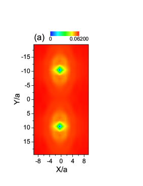
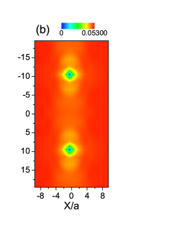
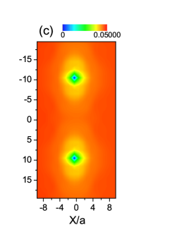
Figure 6: The spatial distributions of the $s$-wave pairing order parameters with the orbital anisotropy $\varepsilon=0.2$. (a) The longitudinal NN pairing $\Delta^{NN}_{L}(\vec{r})$, (b) the transverse NN pairing $\Delta^{NN}_{T}(\vec{r})$, and (c) the NNN $s_{x^{2}y^{2}}$-wave pairing order parameters $\Delta^{NNN}(\vec{r})$. All of them show anisotropy.

In this subsection, we consider the effect of orbital ordering to the vortex lattice states. The band and interaction parameters are the same as in Sec. V.1, except that we add the anisotropy term of Eq. (8) with $\delta\varepsilon=0.2$. Such a term breaks the degeneracy between the $d_{xz}$ and $d_{yz}$-orbitals, and reduces the $C_{4}$ symmetry down to $C_{2}$.

Fig. 6 (a), (b) and (c) depict the spatial distributions of the NN $s_{x^{2}+y^{2}}$-pairing order parameters $\Delta^{NN}_{L}$ and $\Delta^{NN}_{T}$, and the NNN $s_{x^{2}y^{2}}$-pairing order parameters in a magnetic unit cell, respectively. All of them clearly exhibit the breaking of the 4-fold symmetry down to the 2-fold one. For the dominant NN $s_{x^{2}+y^{2}}$-pairings, the coherence lengths along the $x$ and $y$-directions are no longer the same, which can be estimated as $\xi_{x}\approx 3a$ and $\xi_{y}\approx 7a$, respectively. From Fermi surface Fig. 2 (b), in the presence of orbital ordering, the electron pocket in the $y$-direction shrinks, which implies that Cooper pairing superfluid stiffness is weaker along the $y$-direction than the $x$-direction. This picture agrees with the larger value of $\xi_{y}$ exhibiting in Figs. 6.

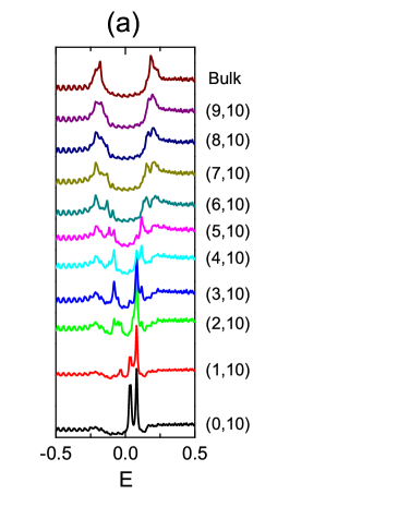
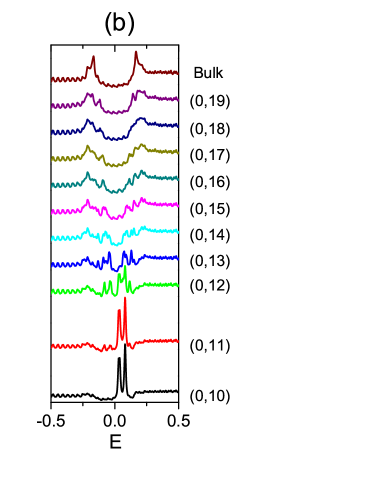
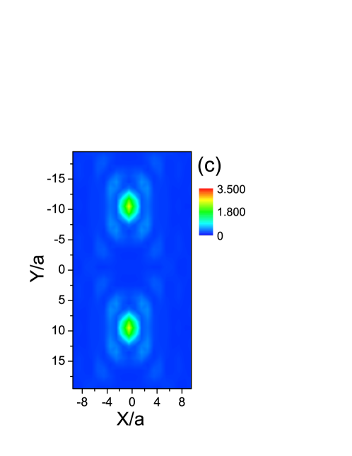
Figure 7: The LDOS v.s. tunneling energy $E$ at different sites from vortex core to outside along (a) the $x$-axis (short axis) and (b) the $y$-axis (long axis). The distances of each site from the vortex core take the step of one lattice constant. (c) The spatial LDOS distributions at the vortex core resonant energy $E_{er}=0.038$ .

Next we turn to study the LDOS patterns for the extended $s_{\pm}$-wave with orbital ordering. In comparison with those without orbital ordering depicted in Fig. 5 (c), the LDOS patterns in Fig. 7 (a) and (b) exhibit significant anisotropy. At the vortex core center, the resonance peak splits into two pieces inside gap. This feature is similar to the previous studies on the $s_{x^{2}y^{2}}$-wave pairing with SDW in iron-based superconductorhu2009 and the $d$-wave pairing with antiferromagnetic ordering in cuprateszhu2001 . Away from the vortex center, however, the peaks of the particle and hole branches along short ($x$) and long ($y$) axes behave differently. The separation between the particle and hole peaks disperses along the short axis much quicker than that along the long axis. The peak intensities along the short axis are stronger than those along the long axis. These features are in good agreement with recent experiment observations song2011 . The pronounced anisotropy also exhibits in the spatial variation of the LDOS at the energy $E_{er}=0.038$ where the resonance peak is located, presented in Fig. 7 (c). Moreover, with negative $\delta\varepsilon$ which loads particles in $d_{xz}$ in prior to $d_{yz}$, all above pictures will have a $\pi/2$-rotation. Therefore, the experimentally observed anisotropy agrees with the picture of orbital ordering.

VI Discussions and Conclusions

We have studied a minimal two-orbital model with orbital ordering to interpret the recent STM observations in Ref. [song2011, ] including the nodal superconductivity and the anisotropy vortex structure in FeSe superconductors. In considering the absence of magnetic long-range-order in FeSe at ambient pressure, orbital ordering provides a natural formalism for anisotropy. The NN $s_{x^{+}y^{2}}$-wave and the NNN $s_{x^{2}y^{2}}$-wave are considered, which generally are mixed. When the NNN pairing dominates, nodal pairing still exists even in the appearance of orbital ordering. We further performed the BdG calculation for the vortex tunneling spectra in the presence of orbital ordering, which breaks $C_{4}$ rotational symmetry down to $C_{2}$ and explicitly induces anisotropic vortex structures.

The microscopic mechanism of the origin of this spontaneous anisotropy remains an open question. It might be related to the strong antiferromagnetic fluctuations. As shown in Ref. [fernandes2012, ; xu2008, ; fang2008, ], before the onset of the antiferromagnetic long rang order, the spin nematic order with a Z₂ symmetry breaking occurs. This nematic order corresponds to anisotropic spin-spin correlation along $a$ and $b$-axis, which can in turn induce orbital ordering.

VII Acknowledgement

C. W. thanks Z. Y. Lu, and F. J. Ma for helpful discussion. H. H. H. and C. W. are partly supported by the NBRPC (973 program) 2011CBA00300 (2011CBA00302), NSF-DMR-1105945 and Sloan Research Foundation. C. L. S., X. C., X. C. M. and Q. K. X. are supported by National Science Foundation and Ministry of Science and Technology of China.

Note added    Near the completion of this manuscript, we learned the article by Chowdhury et al. chowdhury2011 which studied the anisotropic vortex tunneling spectra in Ref. [song2011, ] through the Ginzburg-Landau formalism.

References

- (1) Can-li Song, Yi-lin Wang, Peng Cheng, Ye-ping Jiang, Wei Li, Tong Zhang, Zhi Li, Ke He, Lili Wang, Jin-feng Jia, Hsiang-Hsuan Hung, Congjun Wu, Xucun Ma, Xi Chen, and Qi-kun Xue, Science 332, 1410 (2011).
- (2) Y. Kamihara, T. Watanabe, M. Hirano and H. Nosono, J. Am. Chem. Soc. 130, 3296 (2008).
- (3) C. de la Cruz et al., Nature (London) 453, 899 (2008).
- (4) T. Hanaguri, S. Nittaka, K. Kuroki and H. Takagi, Sceince, 328 (2010).
- (5) X. Zhang, Y. S. Oh, Y. Liu, L. Yan, K. H. Kim, R. L. Greene, and I. Takeuchi, Phys. Rev. Lett. 102, 147002 (2009).
- (6) H. Ding et al., Europhys. Lett. 83, 47001 (2008).
- (7) K. Seo, B. A. Bernevig and J. Hu, Phys. Rev. Lett. 101, 206404 (2008).
- (8) M. Daghofer et al., Phys. Rev. Lett. 101, 237004 (2008); A. Moreo, M. Daghofer, J. A. Riera, and E. Dagotto, Phys. Rev. B 79, 134502 (2009).
- (9) F. Wang, H. Zhai, Y. Ran and A. Vishwanath, D. H. Lee, Phys. Rev. Lett., 102, 047005 (2009).
- (10) V. Cvetkovic and Z. Tesanovic, Europhysics Lett. 85, 37002 (2009).
- (11) V. Cvetkovic and Z. Tesanovic, Phys. Rev. B 80, 024512 (2009).
- (12) M. R. Norman, Physics 1, 21 (2008).
- (13) J. D. Fletcher et al., Phys. Rev. Lett. 102, 147001 (2009).
- (14) C. W. Hicks et al., Phys. Rev. Lett. 103, 127003 (2009).
- (15) B. Zeng, G. Mu, H. Q. Luo, T. Xiang, H. Yang, L. Shan, C. Ren, I. I. Mazin, P. C. Dai and H.-H. Wen, Nat. Comm. 1, 112 (2010).
- (16) I.I. Mazin, D.J. Singh, M.D. Johannes and M.H. Du, Phys. Rev. Lett. 101, 057003 (2008).
- (17) Z.-J. Yao, J.-X. Li and Z. D. Wang, New. J. Phys. 11, 025009 (2009).
- (18) F. Wang, H. Zhai and D. -H. Lee, Phys. Rev. B 81, 184512 (2010).
- (19) Fa Wang, Hui Zhai, Ying Ran, Ashvin Vishwanath and Dung-Hai Lee, Phys. Rev. Lett. 102, 047005 (2009).
- (20) Y. Chen et al., Phys. Rev. B 78, 064515 (2008).
- (21) Chen Fang, Hong Yao, Wei-Feng Tsai, Jiang Ping Hu and Steven A. Kivelson, Phys. Rev. B 77, 224509 (2008).
- (22) Cenke Xu, Markus Muller and Subir Sachdev, Phys. Rev. B 78, 020501(R) (2008).
- (23) Shiliang Li, Clarina de la Cruz, Q. Huang, Y. Chen, J. W. Lynn, Jiangping Hu, Yi-Lin Huang, Fong-chi Hsu, Kuo-Wei Yeh, Maw-Kuen Wu and Pengcheng Dai, Phys. Rev. B 79, 054503 (2009).
- (24) Wei Bao, Y. Qiu, Q. Huang, M.A. Green, P. Zajdel, M.R. Fitzsimmons, M. Zhernenkov, S. Chang, M. Fang, B. Qian, E.K. Vehstedt, J. Yang, H.M. Pham, L. Spinu and Z.Q. Mao, Phys. Rev. Lett. 102, 247001 (2009).
- (25) J. Knolle, I. Eremin, A. Akbari, and R. Moessner, Phys. Rev. Lett. 104, 257001 (2010)
- (26) S. Medvedev et al., Nat. Mater. 8, 630 (2009).
- (27) W. C. Lee and C. Wu, Phys. Rev. B 80, 104438 (2009).
- (28) S. Raghu, A. Paramekanti, E-.A. Kim, R. A. Borzi, S. A. Grigera, A. P. Mackenzie and S. A. Kivelson, Phys. Rev. B 79, 214402 (2009).
- (29) W. C. Lee, D. P. Arovas and C. Wu, Phys. Rev. B 81, 184403 (2010)
- (30) W. C. Lee and C. Wu, Phys. Rev. Lett. 103, 176101 (2009).
- (31) S. Raghu, X. -L. Qi, C. -X. Liu, D. J. Scalapino and S. -C. Zhang, Phys. Rev. B 77, 220503(R) (2008).
- (32) W. -F. Tsai, Y. -Y. Zhang, C. Fang and J. Hu, Phys. Rev. B 80, 064513 (2009).
- (33) T. Zhou, X. Hu, J. -X. Zhu and C. S. Ting, e-print: 0904.4273.
- (34) X. Hu, C. S. Ting and J.-X. Zhu, Phys. Rev. B 80, 014523 (2009).
- (35) H. -M. Jiang, J.- X. Li and Z. D. Wang, Phys. Rev. B 80, 134505 (2009).
- (36) Y. -Y. Zhang et al., Phys. Rev. B 80, 094528 (2009).
- (37) S. Lebegue, Phys. Rev. B 75, 035110 (2007); D. H. Lu et al., Science 455, 81 (2008).
- (38) Frank Krger et al., Phys. Rev. B 79, 054504 (2009).
- (39) C. -C. Lee, W. -G. Yin and W. Ku, Phys. Rev. Lett. 103, 267001 (2009).
- (40) Weicheng Lv, Jiansheng Wu, and Philip Phillips, Phys. Rev. B 80, 224506 (2009).
- (41) C.-C. Chen, J. Maciejko, A. P. Sorini, B. Moritz, R. R. P. Singh and T. P. Devereaux, Phys. Rev. B 82, 100504(R) (2010).
- (42) Weicheng Lv, Frank Krger and Philip Phillips, Phys. Rev. B 82, 045125 (2010).
- (43) Weicheng Lv and Philip Phillips, Phys. Rev. B 84, 174512 (2011).
- (44) Qiang Han, J. Phys.: Condens. Matter 22, 035702 (2010).
- (45) F. Yang, H. Zhai, F. Wang and D. -H. Lee, Phys. Rev. B 83, 134502 (2011).
- (46) Can-li Song, Yi-lin Wang, Peng Cheng, Ye-ping Jiang, Wei Li, Tong Zhang, Zhi Li, Ke He, Lili Wang, Jin-feng Jia, Hsiang-Hsuan Hung, Congjun Wu, Xucun Ma, Xi Chen, and Qi-kun Xue, Supporting Online Material in Science 332, 1410 (2011).
- (47) Y. Gao et al., Phys. Rev. Lett. 106, 027004 (2011).
- (48) J.-X. Zhu and C. S. Ting, Phys. Rev. Lett. 87, 147002 (2001).
- (49) D. Chowdhury, E. Berg, and S. Sachdev, Phys. Rev. B 84, 205113 (2011).
- (50) R. M. Fernandes, A. V. Chubukov, J. Knolle, and I. Eremin, and J. Schmalian, Phys. Rev. B 85, 024534 (2012)