Improved multiscale computational strategies for delamination

1 Introduction

The virtual testing of delamination is a goal shared by many practitioners, especially in the aeronautical field. In order to reach such an objective, two research topics which have undergone drastic changes over the last twenty years must be linked: the relevant modeling of composites and the efficient analysis of structures.

Indeed, there have been many advances toward a better understanding of the mechanics of laminated composites and the mechanisms of damage. The validity of two types of models, microscale models and mesoscale models, has been proven. Microscale models are closely connected to the physics of the material and, thus, provide a reliable framework for simulation. They take into account many damage processes, such as diffuse intralaminar degradations percolating into transverse cracking, diffuse interface degradations leading to distributed delamination, chemically- or thermally-induced degradations, or fiber breakage. [12, 8]. On the microscale, simulations can combine continuous (damage) and discrete (fracture) degradation models [18]. Unfortunately, the analysis of models defined on the microscale requires such a refined discretization that only small test specimens can be simulated. Industrial-size structural calculations are beyond the reach of even recent computers. Mesomodels [1, 13, 3] are defined on a scale which makes both the introduction of physics-based components and the simulation of small industrial structures possible. Very often these models rely on the definition of two mesoconstituents, the ply (a three-dimensional entity) and the interface (a two-dimensional entity), which are modeled using continuum (damage) mechanics and behavior derived from the homogenization of micromodels [17, 16]. Nevertheless, in order to achieve reliable simulations, refined discretizations are still required for the correct representation of the stress gradients induced by edge effects, which are responsible for the initiation of many degradations. Therefore, the resulting problems remain very large (in terms of the number of degrees of freedom) and highly nonlinear, which creates potential instabilities.

In a first approach to the reliable simulation of delamination in composite structures, we chose to neglect the effect of damage within plies and concentrate on the degradations at the interfaces. Thus, we adopted the mesomodel presented in [1], in which the debonding phenomenon is localized at the interfaces and handled through cohesive behavior. A similar approach with a different interface behavior (degradations based on plasticity) was applied in [22].

In order to handle the large nonlinear systems associated with this modeling approach, one can consider using one of the several multiscale [19, 5, 4, 14] and enrichment [21, 10, 6, 20] techniques developed recently. We based our strategy on the mixed domain decomposition method described in [14], which places special emphasis on the interfaces between substructures. Consequently, the reference problem resulting from the mesomodel chosen is substructured by nature, and the cohesive interfaces of the model are handled within the interfaces of the domain decomposition method. This idea is developed in Section 2. Furthermore, the resolution of the substructured problem by a LATIN iterative solver has very advantageous numerical properties: the nonlinearities are dealt with through local problems, and very little matrix reassembling is required. The incremental micro-macro LATIN algorithm as a resolution strategy for delamination problems is presented in Section 2.2. As shown in Section 2.3, the direct application of this method leads to a number of numerical difficulties. A first issue occurs when setting the parameters of the method: in Section 3, we present the indispensable tuning of the search directions according to the interface’s status. Subsequently, the main remaining difficulties concern the treatment of the macroscale of the problem. In this paper, the emphasis is on the adaptation of our strategy in order to deal with large macroproblems. (Important remarks on how to make the macroproblem more relevant can be found in [11].) In Section 4, we present the parallelization of the resolution, which was inspired by [19]. In order to do that, we introduce a third level of discretization after the first and most refined level (the finite element) and the second level (the substructure): interconnected substructures are combined into “super-substructures” (which fill up the memory capacity of processors) connected to one another through “super-interfaces” using Message Passing Interface (MPI). The method is validated in Section 5 using a complex test case. The handling of the instabilities is not described in this paper. The interested reader may refer to [11] where the adaptation of an arc-length algorithm with local control is presented.

2 Application of the two-scale domain decomposition strategy to delamination analysis

2.1 The substructured delamination problem

Let us consider a laminated structure $\mathbf{E}$ defined in a domain $\Omega$ bounded by $\partial\Omega$ and consisting of $N_{P}$ adjacent plies $P$, each defined in a domain $\Omega_{P}$, with $\Omega=\bigcup_{P}\Omega_{P}$. Adjacent plies $P$ and $P^{\prime}$ are joined by cohesive interfaces $I_{PP^{\prime}}$. An external traction field $\underline{F}_{d}$ is prescribed over a part $\partial\Omega_{f}$ of $\Omega$, and a displacement field $\underline{U}_{d}$ is prescribed over the complementary part $\partial\Omega_{u}$ of $\Omega$. Let $\underline{n}_{P}$ denote the outer normal to the boundary $\partial\Omega_{P}$ of Ply P, $\underline{f}_{d}$ the volume force, $\underline{\underline{\sigma}}$ the Cauchy stress tensor and $\underline{\underline{\epsilon}}$ the symmetric part of the displacement gradient. The simulation is performed using a classical incremental scheme, assuming small perturbations and quasi-static isothermal evolution over time.

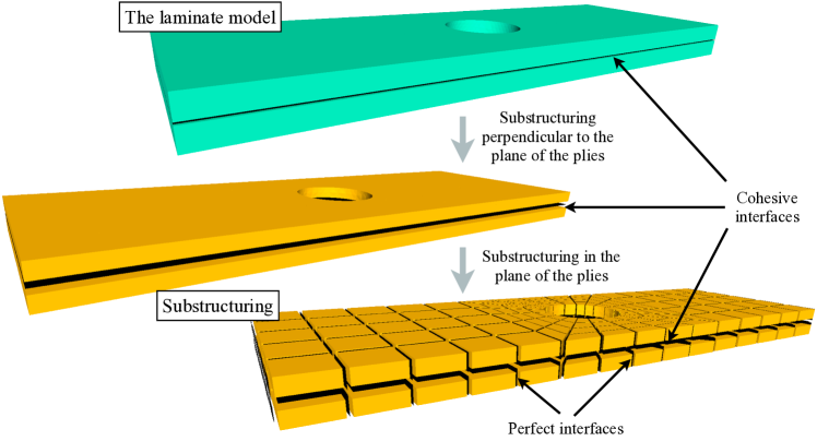
Figure 1: Decomposition of the laminated composite structure into substructures

The laminated structure $\mathbf{E}$ is decomposed into substructures and interfaces as shown in Fig. 1. Each of these mechanical entities has its own kinematic and static unknown fields as well as its own constitutive law. The substructuring pattern is defined in such a way that the domain decomposition interfaces coincide with the material’s cohesive interfaces, so that each substructure belongs to a unique ply $P$ and has a constant linear constitutive law. A substructure $E$ defined in Domain $\Omega_{E}$ is connected to an adjacent substructure $E^{\prime}$ through an interface $\Gamma_{EE^{\prime}}=\partial\Omega_{E}\cap\partial\Omega_{E^{\prime}}$ (Fig. 2). The surface entity $\Gamma_{EE^{\prime}}$ applies force distributions $\underline{F}_{E}$, $\underline{F}_{E^{\prime}}$ and displacement distributions $\underline{W}_{E}$, $\underline{W}_{E^{\prime}}$ to $E$ and $E^{\prime}$. Let $\Gamma_{E}=\bigcup_{E^{\prime}\in\mathbf{E}}\Gamma_{EE^{\prime}}$. Over a substructure $E$ such that $\Gamma_{E}\cap\partial\Omega\neq\emptyset$, the boundary condition $(\underline{U}_{d},\underline{F}_{d})$ is applied through a boundary interface $\Gamma_{E_{d}}$.

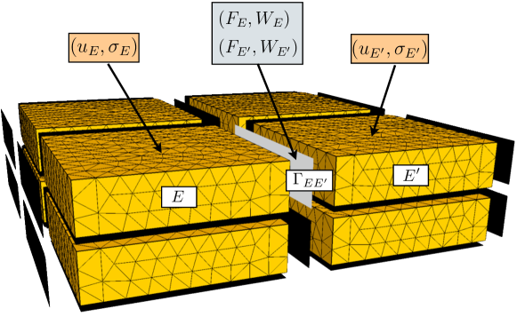
Figure 2: Decomposition of the laminated composite structure into substructures: mixed unknown fields

At each step of the incremental time resolution algorithm, the substructured quasi-static problem consists in finding $s=(s_{E})_{E\in\mathbf{E}}$ (where $s_{E}=(\underline{u}_{E},\underline{W}_{E},\underline{\underline{\sigma}}_{E},\underline{F}_{E})$) which is a solution of the following equations:

• kinematic admissibility of Substructure $E$:

  $$\textrm{at each point of }\Gamma_{E},\quad{\underline{u}_{E}}={\underline{W}_{E}}$$ (1)

• static admissibility of Substructure $E$:

  $$\begin{array}[]{l}\displaystyle\forall({\underline{u}_{E}}^{\star},{\underline{W}_{E}}^{\star})\in\mathcal{U}_{E}\times\mathcal{W}_{E}\ /\ {{\underline{u}_{E}}^{\star}}_{|\partial\Omega_{E}}={{\underline{W}_{E}}^{\star}},\\ \begin{array}[]{ll}\displaystyle\int_{\Omega_{E}}Tr\left(\underline{\underline{\sigma}}_{E}\,\underline{\underline{\epsilon}}({\underline{u}_{E}}^{\star})\right)\ d&\Omega=\displaystyle\int_{\Omega_{E}}\underline{f}_{d}.{\underline{u}_{E}}^{\star}\,d\Omega\\ &+\displaystyle\int_{\partial{\Gamma_{E}}}\underline{F}_{E}.{\underline{W}_{E}}^{\star}\ d\Gamma\end{array}\end{array}$$ (2)

• linear orthotropic constitutive law of Substructure $E$:

  $$\textrm{at each point of }\Omega_{E},\quad\underline{\underline{\sigma}}_{E}=\mathbf{K}\,\underline{\underline{\epsilon}}(\underline{u}_{E})$$ (3)

• behavior of the interfaces $\Gamma_{EE^{\prime}}\in\Gamma_{E}$:

  $$\begin{array}[]{l}\displaystyle\textrm{at each point of }\Gamma_{EE^{\prime}}\in\Gamma_{E},\\ \displaystyle R_{EE^{\prime}}(\underline{W}_{E},\underline{W}_{E^{\prime}},\underline{F}_{E},\underline{F}_{E^{\prime}})=0\end{array}$$ (4)

• behavior of the interfaces at the boundary $\partial\Omega\cap\Gamma_{E}$:

  $$\begin{array}[]{c}\textrm{at each point of }\Gamma_{{E}_{d}},\quad R_{Ed}(\underline{W}_{E},\underline{F}_{E})=0\\ (\underline{W}_{E}=\underline{u}_{d}\text{ on }\partial\Omega_{u}\text{ and }\underline{F}_{E}=\underline{F}_{d}\text{ on }\partial\Omega_{f})\end{array}$$ (5)

We make the formal relation $R_{EE^{\prime}}=0$ explicit in the two cases we will be considering:

• perfect interface:

  $$\left\{\begin{array}[]{l}\underline{F}_{E}+\underline{F}_{E^{\prime}}=0\\ \underline{W}_{E}-\underline{W}_{E^{\prime}}=0\end{array}\right.$$ (6)

• cohesive interface:

  $$\left\{\begin{array}[]{l}\displaystyle\underline{F}_{E}=\underline{\underline{K}}_{P}(\underline{[W]}_{EE^{\prime}}(\tau<t)).\underline{[W]}_{EE^{\prime}}\\ \displaystyle\underline{F}_{E}+\underline{F}_{E^{\prime}}=0\\ \end{array}\right.$$ (7)

  where $\underline{[W]}_{EE^{\prime}}=\underline{W}_{E^{\prime}}-\underline{W}_{E}$. The stiffness operator $\underline{\underline{K}}_{P}$ can be expressed in the $(\underline{N}_{1},\underline{N}_{2},\underline{n}_{P})$ basis as (Fig. 3):

  $$\left(\begin{array}[]{ccc}\displaystyle(1-d_{1}){k_{1}}^{0}&0&0\\ 0&\displaystyle(1-d_{2}){k_{2}}^{0}&0\\ 0&0&\displaystyle\left(1-h_{+}\underline{[W]}_{EE^{\prime}}\ d_{3}\right){k_{3}}^{0}\end{array}\right)$$ (8)

  where $h_{+}$ is the positive indicator function.

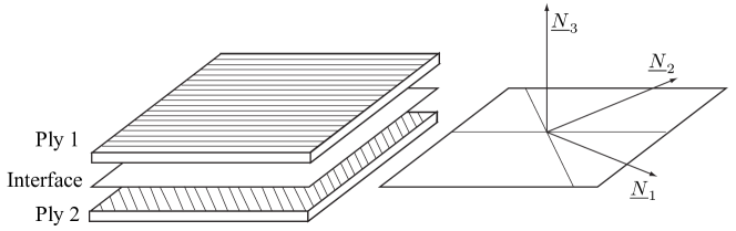
Figure 3: The components of the mesomodel

The cohesive constitutive law of an interface joining two adjacent plies is described classically through continuum damage mechanics. Local damage variables $({d_{i}})_{i\in[1\ 3]}$, with values ranging from $0$ (healthy interface) to $1$ (completely damaged interface), are introduced into the interface model in order to simulate its progressive softening. The parameters $(d_{i})_{i\in[1\ 3]}$ are related to the local energy release rates $(Y_{i})_{i\in[1\ 3]}$ of the interface’s degradation modes (traction along Direction $\underline{N}_{3}$ and shear along Directions $\underline{N}_{1}$ and $\underline{N}_{2}$).

$$Y_{i}=-\frac{\partial e_{d}}{\partial d_{i}}\qquad\textrm{where}\quad\left\{\begin{array}[]{ccl}Y_{1}&=&\displaystyle\frac{1}{2}k_{1}\left(\underline{[W]}_{EE^{\prime}}.\underline{N}_{1}\right)^{2}\\ Y_{2}&=&\displaystyle\frac{1}{2}k_{2}\left(\underline{[W]}_{EE^{\prime}}.\underline{N}_{2}\right)^{2}\\ Y_{3}&=&\displaystyle\frac{1}{2}k_{3+}\left(\underline{[W]}_{EE^{\prime}}.\underline{N}_{3}\right)_{+}^{2}\end{array}\right.$$ (9)

The damage variables are assumed to be functions of a single quantity: the maximum over time $Y_{|t}$ of a combination of the energy release rates ${({Y_{i}}_{|\tau})}_{i\in[1\ 3],\ \tau\leqslant t}$:

$$Y_{|t}=sup_{(\tau\leq t)}\left({Y_{3}}_{|\tau}^{\alpha}+\gamma_{1}{Y_{1}}_{|\tau}^{\alpha}+\gamma_{2}{Y_{2}}_{|\tau}^{\alpha}\right)^{\frac{1}{\alpha}}$$ (10)

The evolution laws express that:

$$d_{1}=d_{2}=d_{3}=w(Y)\quad\textrm{where, in general,}\quad w(Y)=\frac{n}{n+1}\left(\frac{Y}{Y_{c}}\right)^{n}$$ (11)

$n$ and $\alpha$ being scalar parameters of the model. When Parameters $\gamma_{1}$ and $\gamma_{2}$ are set to identified physical values such that $\gamma_{1}\neq\gamma_{2}\neq 1$, the energies dissipated during the propagation of the crack are different for the three modes. Details on the identification procedure for such a model can be found in [2].

After a cohesive interface has become fully damaged, it is converted into a (frictionless) contact interface.

2.2 Two-scale iterative resolution of the substructured problem

2.2.1 Introduction of the macroscopic scale

In the end, the substructured problem defined in the previous section will be solved using an iterative LATIN algorithm, which will be described in the next section. In order to ensure the scalability of the strategy, a coarse global problem, associated with the equilibrium and continuity of what one calls the “macro” force and displacement fields at the interfaces, must be solved at each iteration.

Over each interface $\Gamma_{EE^{\prime}}$ such that $(E,E^{\prime})\in\mathbf{E}^{2}$, the interface fields are divided into a macro part (superscript $M$) and a micro part (superscript $m$). The macro part belongs to a small subspace (9 macro degrees of freedom per plane interface for a 3D problem).

$$\begin{array}[]{l}\displaystyle{\underline{F}_{E}}=\underline{F}_{E}^{M}+\underline{F}_{E}^{m}\\ \displaystyle{\underline{W}_{E}}=\underline{W}_{E}^{M}+\underline{W}_{E}^{m}\end{array}$$ (12)

The macro and micro data are uncoupled with respect to the interface’s virtual work:

$$\begin{array}[]{l}\displaystyle\forall\displaystyle(\underline{F}_{E},\underline{W}_{E})\in\mathcal{F}_{E}\times\mathcal{W}_{E},\\ \displaystyle\int_{\Gamma_{EE^{\prime}}}\underline{F}_{E}.\underline{W}_{E}\ d\Gamma=\int_{\Gamma_{EE^{\prime}}}\underline{F}_{E}^{M}.\underline{W}_{E}^{M}\ d\Gamma+\int_{\Gamma_{EE^{\prime}}}\underline{F}_{E}^{m}.\underline{W}_{E}^{m}\ d\Gamma\end{array}$$ (13)

Each macrospace is defined by one’s choice of its basis. Numerical tests have shown that the use of a linear macro basis gives the method good scalability properties. Indeed, the corresponding macrospace includes the part of the interface fields with the largest wavelength. Consequently, according to Saint-Venant’s principle, the micro complement resulting from the iterative resolution of the local problems has only a local influence.

2.2.2 The iterative algorithm

Here, the iterative LATIN algorithm for the resolution of nonlinear problems is applied to the resolution of the substructured reference problem, the nonlinearities being localized in the (cohesive) interfaces.

The equations of the problem can be divided into two groups:

• linear equations in substructure variables and interface macroscopic variables:

  • static admissibility of the substructures

  • kinematic admissibility of the substructures

  • linear constitutive law of the substructures

  • linear equilibrium of the macro interface forces

• local equations in interface variables:

  • behavior of the interfaces

The solutions $\displaystyle s=(s_{E})_{E\in\mathbf{E}}=(\underline{u}_{E},\underline{W}_{E},\underline{\underline{\sigma}}_{E},\underline{F}_{E})_{E\in\mathbf{E}}$ of the first set of equations belong to Space $\mathbf{A_{d}}$ and the solutions $\displaystyle\widehat{s}=(\widehat{s}_{E})_{E\in\mathbf{E}}=(\underline{\widehat{u}}_{E},\underline{\widehat{W}}_{E},\underline{\underline{\widehat{\sigma}}}_{E},\underline{\widehat{F}}_{E})_{E\in\mathbf{E}}$ of the second set of equations belong to $\boldsymbol{\Gamma}$. The converged solution $s_{ref}$ is such that:

$$s_{ref}\in\mathbf{A_{d}}\bigcap\boldsymbol{\Gamma}$$ (14)

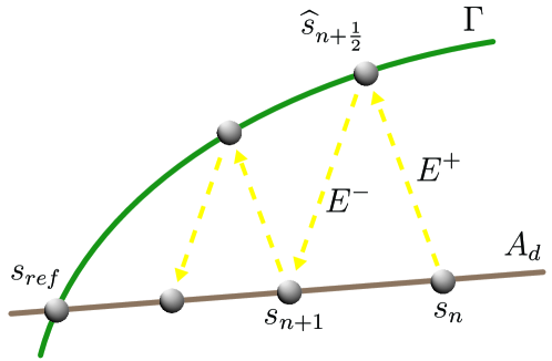
Figure 4: Illustration of the LATIN iterative algorithm

The resolution process consists in seeking the solution $s_{ref}$ alternatively in these two spaces: first, a solution $s_{n}$ is found in $\mathbf{A_{d}}$, then a solution $\widehat{s}_{n+\frac{1}{2}}$ is found in $\boldsymbol{\Gamma}$. In order for the two problems to be well-posed, one introduces two search directions, $\mathbf{E^{+}}$ and $\mathbf{E^{-}}$, linking the solutions $s$ and $\widehat{s}$ through the iterative process (see Fig. 4). Hence, an iteration of the LATIN algorithm consists of two stages:

• a local stage:

  $$\textit{Find}\ \widehat{s}_{n+\frac{1}{2}}\in\boldsymbol{\Gamma}\ \textit{such that}\ \left(\widehat{s}_{n+\frac{1}{2}}-s_{n}\right)\in\mathbf{E^{+}}$$ (15)

• and a linear stage:

  $$\textit{Find}\ s_{n+1}\in\mathbf{A_{d}}\ \textit{such that}\ \left(s_{n+1}-\widehat{s}_{n+\frac{1}{2}}\right)\in\mathbf{E^{-}}$$ (16)

In the following sections, the subscript $n$ will be omitted.

The local stage

During the local stage, uncoupled problems are solved at each point of the interfaces $(\Gamma_{EE^{\prime}})_{|(E,E^{\prime})\in\mathbf{E}^{2}}$ (as well as $(\Gamma_{E_{d}})_{E\in\mathbf{E}}$ for the interfaces which belong to the boundary $\partial\Omega$):

$$\begin{array}[]{l}\textit{Find}\ (\underline{\widehat{F}}_{E},\underline{\widehat{W}}_{E},\underline{\widehat{F}}_{E^{\prime}},\underline{\widehat{W}}_{E^{\prime}})\vspace{0.2cm}\textit{ such that: }\\ \left\{\begin{array}[]{l}\displaystyle\mathcal{R}_{EE^{\prime}}(\underline{\widehat{F}}_{E},\underline{\widehat{W}}_{E},\underline{\widehat{F}}_{E^{\prime}},\underline{\widehat{W}}_{E^{\prime}})=0\\ \displaystyle(\underline{\widehat{F}}_{E}-\underline{F}_{E})-k^{+}(\underline{\widehat{W}}_{E}-\underline{W}_{E})=0\\ \displaystyle(\underline{\widehat{F}}_{E^{\prime}}-\underline{F}_{E^{\prime}})-k^{+}(\underline{\widehat{W}}_{E^{\prime}}-\underline{W}_{E^{\prime}})=0\end{array}\right.\end{array}$$ (17)

The last two equations of this system define the search direction $E^{+}$ ($k^{+}$ and $k^{-}$ are scalar search direction which, physically, are analogous to “stiffnesses”). In the case of a cohesive interface, Problem (17) is nonlinear and its solution is obtained through a Newton-Raphson scheme.

The linear stage

The linear stage consists in the resolution of a series of linear systems within the substructures under the constraint of macroscopic equilibrium of the interface forces.

$$\text{at Interface }{\Gamma_{EE^{\prime}}}_{|(E,E^{\prime})\in\mathbf{E}^{2}},\quad\underline{F}_{E}^{M}+\underline{F}_{E^{\prime}}^{M}=0$$ (18)

In order to verify the macroscopic condition exactly and the search direction $E^{-}$ defined in (16) as well as possible, we use a Lagrangian formulation, which leads to:

$$\begin{array}[]{ll}\displaystyle\forall\underline{W}_{E}^{\star}\in\mathcal{W}_{E},&\displaystyle\quad\int_{\Gamma_{E}}\left(\underline{F}_{E}-\underline{\widehat{F}}_{E}\right).{\underline{W}_{E}}^{\star}\ d\Gamma\\ &\displaystyle+\int_{\Gamma_{E}}\left(k^{-}\ (\underline{W}_{E}-\underline{\widehat{W}}_{E})-k^{-}\underline{\widetilde{W}}^{M}\right).{\underline{W}_{E}}^{\star}\ d\Gamma=0\end{array}$$ (19)

which can be viewed as a modified search direction, the Lagrange multiplier $\underline{\widetilde{W}}^{M}$ becoming an additional unknown of Interface $\Gamma_{EE^{\prime}}$.

The problem which needs to be solved for each substructure $E$ is obtained by substituting (19) into (2):

$$\begin{array}[]{l}\displaystyle\forall(\underline{u}_{E}^{\star},\underline{W}_{E}^{\star})\in{\mathcal{U}_{E}}\times{\mathcal{W}_{E}},\\ \displaystyle\int_{\Omega_{E}}Tr(\underline{\underline{\epsilon}}(\underline{u}_{E})\,K\underline{\underline{\epsilon}}({\underline{u}_{E}}^{\star}))\ d\Omega+\int_{\Gamma_{E}}k^{-}\,\underline{W}_{E}.{\underline{W}_{E}}^{\star}\ d\Gamma\\ \displaystyle=\int_{\Omega_{E}}\underline{f}_{d}.{\underline{u}_{E}}^{\star}\,d\Omega+\int_{\Gamma_{E}}(\underline{\widehat{F}}_{E}+k^{-}\underline{\widehat{W}}_{E}+k^{-}{\underline{\widetilde{W}}}^{M}).{\underline{W}_{E}}^{\star}\ d\Gamma\end{array}$$ (20)

The condensation of this equation onto the macro degrees of freedom leads to a relation between $\underline{F}_{E}^{M}$ and $\underline{\widetilde{W}}_{E}^{M}$ which can be introduced into the macro equilibrium equation (18). Finally, one gets a small linear system defined in the macro degrees of freedom. All the subdomains contribute to that “global” system through homogenized (condensed) flexibilities $\mathbb{L}_{E}^{M}$ calculated explicitly.

$$\begin{array}[]{ll}\displaystyle\forall&\displaystyle\underline{\widetilde{W}}^{M\star}\in{\mathcal{W}^{M}},\quad\sum_{E}\int_{\Gamma_{E}}\mathbb{L}_{E}^{M}\ \underline{\widetilde{W}}^{M}.\underline{\widetilde{W}}^{M\star}\ d\Gamma\\ &\displaystyle=\sum_{E}\int_{\partial\Omega_{f}}\underline{F}_{d}.\underline{\widetilde{W}}^{M\star}\ d\Gamma-\sum_{E}\int_{\Gamma_{E}}\underline{\widetilde{F}}_{E}.\underline{\widetilde{W}}^{M\star}\ d\Gamma\end{array}$$ (21)

The macroscopic problem is discrete by nature and is expressed in matrix form as $\displaystyle\mathbf{L}^{M}\ \widetilde{W}^{M}=F^{M}$, where $\widetilde{W}^{M}$ is the vector of the components of the Lagrange multiplier in the macro basis.

The right-hand side of Equation (21) can be viewed as a macroscopic static residual from the calculation of a single-scale linear stage. In order to derive this term, Problem (20) must be solved independently within each substructure. The resolution of the macroscopic problem (21) leads globally to the Lagrange multiplier $\underline{\widetilde{W}}^{M}$, which is finally used as a prescribed displacement for the resolution of the substructure-independent problems (20).

In order to carry out the resolutions of (20) in substructure variables, one uses the finite element method. Since the constitutive law of the substructures is linear, the stiffness operator of each substructure can be factorized once at the beginning of the calculation and reused without modifications throughout the analysis, which makes the method numerically advantageous.

Algorithm 1 summarizes the iterative procedure described in this section.

Construction of each substructure’s operators ;

Calculation of each substructure’s macro homogenized behavior $\mathbb{L}_{E}^{M}$ ;

Global assembly of the macroscopic operator;

Initialization $s_{0}\in\boldsymbol{\Gamma}$;

for $n=0,\ldots,N$ do

      Linear stage: calculation of $s_{n}\in\mathbf{A_{d}}$ ;

       $\quad\square$ Calculation of the macroscopic right-hand term $\widetilde{F}_{E}$ for each substructure ;

       $\quad\square$ Global assembly of the macroscopic right-hand term ;

       $\quad\square$ Resolution of the macro problem ;

       $\quad\square$ Resolution of the micro problems ;

       Local stage: calculation of $s_{n+\frac{1}{2}}\in\boldsymbol{\Gamma}$ ;

       $\quad\square$ Resolution of the local problems at the boundary interfaces $(\Gamma_{cl})_{E\in\mathbf{E}}$ ;

       $\quad\square$ Resolution of the local problems at the interfaces $(\Gamma_{EE^{\prime}})_{(E,E^{\prime})\in\mathbf{E}^{2}}$;

       Calculation of a global error indicator

end for

Algorithm 1 The two-scale domain decomposition solver

2.3 First example of a delamination analysis

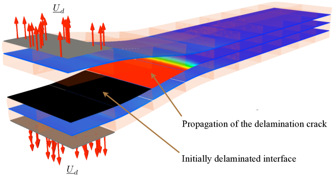
Figure 5: The four-ply DCB test example

A first example of quasi-static delamination analysis is shown in Fig. 5. The structure is a $[0\ 90]_{s}$ double cantilever beam (DCB). The loading leading to Mode-I quasi-static propagation of the crack is increased linearly through ten time steps, the first two corresponding to the initiation of the delamination and the remainder to the crack’s propagation.  

The calculations were performed using a C++ implementation of the mixed domain decomposition method capable of handling the quasi-static analysis of 3D nonlinear problems. In this code, the parallel computations use the MPI library to exchange data among several processors. Each processor is assigned a set of connected substructures and their interfaces; then it calculates the associated operators and solves the local problems (Fig. 8). The allocation of the substructures among the CPUs is handled by a METIS routine. The resolution of the macroproblem does not take full advantage of the parallelism because the substructures send their contributions to the macro problem to a separate processor in which the matrix is assembled and factorized and the substitutions are performed.  

The direct use of the multiscale domain decomposition strategy to simulate the DCB case led to a number of numerical difficulties:

• The convergence rate of the LATIN-based strategy is highly dependent on the residual stiffnesses of the cohesive interfaces as well as the values of the search direction parameters. The iterative solver is even likely to stall when using low values of the search direction parameters. In the next section, we will briefly describe a practical tuning algorithm for the strategy which guarantees convergence.

• The method looses its numerical scalability when the crack’s tip propagates. This phenomenon appears clearly in Fig. 6 under the label “No subresolution”. When the delamination process propagates (time steps 3 to 10), the number of LATIN iterations required for convergence becomes very large. A solution to this problem, described in [11], enabled us to recover the scalability of the method for our test case (under the label “Subresolutions”). This approach, which still needs to be generalized, is based on a filtering of the long-range effects of the crack’s tip achieved through the resolution, at each global LATIN iteration, of local nonlinear problems in a box surrounding the front (where the main sources of nonlinearities are located).

• In this case, the ratio of the number of microscopic DOFs to the number of macroscopic DOFs is relatively small (40). The direct resolution of the macroscopic problem would become an issue if one were addressing the simulation of a realistic composite structure. A solution to this problem is discussed in Section 4.

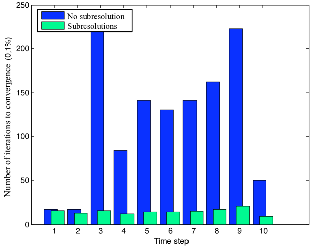
Figure 6: Subiterations near the crack’s tip

3 Analysis of the parameters of the iterative algorithm

A necessary condition for the algorithm to converge is for the search direction parameters $k^{+}$ and $k^{-}$ to be positive definite, symmetrical operators. Previous studies have shown that there exists an optimum set of these operators. However, the optimum values are known to be difficult to interpret when the interface constitutive laws are complex, and even in simplified cases (perfect interfaces) are expensive to calculate. Therefore, our objective was to derive an efficient scalar approximation of these search direction operators for debonding analysis purposes.

As explained in [11], the non-monotonic relation between the interface stresses and the displacement gap due to damage imposes restrictions on the choice of Parameter $k^{+}$. Concerning $k^{-}$, optimum values for a given damage map can be found after a micro/macro decomposition of this operator. Since the status of the interfaces changes with the evolution of the delamination (from elastic to damaged, then from damaged to ruined), the search direction parameters need to be updated often in order to remain optimum. Therefore, parameters whose efficiency range when they are not optimum is broad enough to require less frequent updating are preferred. An effective practical choice is the following:

• Parameter $k^{+}$: in order to avoid stalling or divergence of the algorithm, this parameter is set to a very high value (i.e. the search direction $E^{+}$ is quasi-infinitely stiff).

• Parameter $k^{-}$:

  • perfect interfaces: $k^{-}$ is set to the classically recommended value $E/L$ [14], where $E$ is the Young’s modulus of the adjacent substructure and $L$ a characteristic length of the interface.

  • interfaces with prescribed forces (respectively displacements): $k^{-}$ is set to a very small (respectively large) value in order to enforce the boundary condition through penalization in the adjacent substructure.

  • cohesive interfaces: $k^{-}$ is set to the stiffness of the undamaged interface.

  • delaminated interfaces: $k^{-}$ is set to zero in the shear direction. In the normal direction, $k^{-}$ is set to zero in traction and to the initial stiffness in compression. Therefore, the status of the interface must be checked regularly (e.g. every ten iterations).

The use of an infinitely stiff search direction $E^{+}$ and of the initial cohesive interface stiffness as the search direction parameter $E^{-}$ brings us back to a well-known situation. The algorithm can be viewed as a secant Newton algorithm in which the solutions of the prediction steps are in equilibrium only in the macroscopic space, the equilibrium of the microscopic quantities being achieved at convergence.

4 The three-scale domain decomposition strategy

The decomposition into substructures described in Section 2 leads to a very large macro problem and an unnecessarily refined macroscopic solution. In order to solve large problems such as that represented in Fig. 7, one must place the emphasis on the parallel resolution of the macroproblem and on the selection and transmission of the large-wavelength part of the macroscopic solution.

These two features can be introduced into the method by using any Schur-complement-based domain decomposition technique [7]. We chose to solve the macroproblem using the BDD method [19, 15].

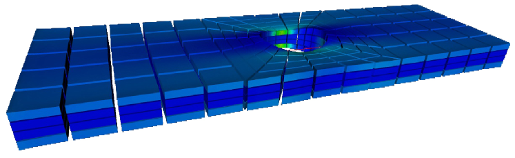
(a) Stresses and displacements in the substructures

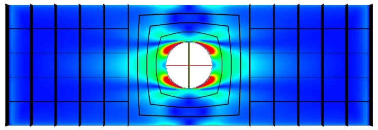
(b) Damage over the upper interface

Figure 7: The four-ply perforated plate problem (3.4 MDOFs)

4.1 Resolution of the macroproblem through the balancing domain decomposition method

4.1.1 Partitioning of the macroproblem

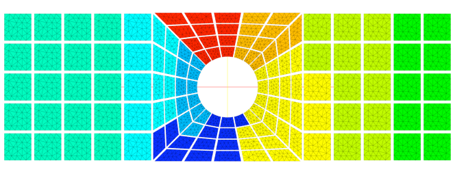
Figure 8: Three-level substructuring: assignment of substructures to processors

The substructures of the initial partitioned problem are grouped into super-substructures ($\bar{E}$) separated by super-interfaces $\Gamma_{\bar{E}\bar{E^{\prime}}}$ (Fig. 8). The algebraic problem to be solved within each of these super-substructures (dropping Superscript $M$) is:

$$\left\{\begin{array}[]{c}\left(\begin{array}[]{cc}\displaystyle\mathbf{L}_{ii}^{(\bar{E})}&\displaystyle\mathbf{L}_{ib}^{(\bar{E})}\\ \displaystyle\mathbf{L}_{bi}^{(\bar{E})}&\displaystyle\mathbf{L}_{bb}^{(\bar{E})}\end{array}\right)\left(\begin{array}[]{c}\displaystyle\widetilde{W}_{i}^{(\bar{E})}\\ \displaystyle\widetilde{W}_{b}^{(\bar{E})}\end{array}\right)=\left(\begin{array}[]{c}\displaystyle F_{i}^{(\bar{E})}\\ \displaystyle F_{b}^{(\bar{E})}+\widetilde{\lambda}_{b}^{(\bar{E})}\end{array}\right)\\ \widetilde{W}_{b}^{(\bar{E})}={\mathbf{A}^{(\bar{E})}}^{T}\underline{\widetilde{W}}_{b}\\ \displaystyle\sum_{\bar{E}}\mathbf{A}^{(\bar{E})}\widetilde{\lambda}_{b}^{(\bar{E})}=0\end{array}\right.$$ (22)

where Subscripts $b$ and $i$ refer respectively to the super-interface quantities and to the internal quantities of the super-substructures. $\mathbf{A}^{(\bar{E})}$ is a Boolean operator which localizes data in such a way that the second equation of System (22) expresses the continuity of the kinematic unknowns (deduced from a single unknown $\underline{\widetilde{W}}_{b}$), while the third equation expresses the equilibrium of the nodal reactions at the super-interfaces.

First, the local equilibrium is condensed onto the super-interfaces by introducing the Schur complement $\mathbf{S}^{(\bar{E})}$ and the condensed force $\underline{F}_{c}^{(\bar{E})}$. The assembled condensed problem becomes:

$$\mathbf{S}\ \underline{\widetilde{W}}_{b}=\underline{F}_{c}$$ (23)

$$\textrm{where}\quad\left\{\begin{array}[]{l|l}\displaystyle\mathbf{S}=\sum_{\bar{E}}\mathbf{A}^{(\bar{E})}\mathbf{S}^{(\bar{E})}{\mathbf{A}^{(\bar{E})}}^{T}\underline{\widetilde{W}}_{b}&\displaystyle\mathbf{S}^{(\bar{E})}=\mathbf{L}_{bb}^{(\bar{E})}-\mathbf{L}_{bi}^{(\bar{E})}\ \mathbf{L}_{ii}^{{(\bar{E})}^{-1}}\ \mathbf{L}_{ib}^{(\bar{E})}\\ \ \displaystyle F_{c}=\sum_{\bar{E}}\mathbf{A}^{(\bar{E})}\underline{F}_{c}^{(\bar{E})}&\displaystyle F_{c}^{(\bar{E})}=F_{b}^{(\bar{E})}-\mathbf{L}_{bi}^{(\bar{E})}\ \mathbf{L}_{ii}^{{(\bar{E})}^{-1}}F_{i}^{(\bar{E})}\end{array}\right.$$

This substructuring technique can be used exactly as in [9] in order to bind a domain which is prone to localization and damage to an undamaged region. Nevertheless, for large interface problems such as those encountered in our case, the condensed problem is much too large to be solved directly, and iterative solvers must be used.

4.1.2 Resolution of the super-interface problem

The condensed macroproblem is solved iteratively using a conjugate gradient algorithm. Classically, this resolution involves only matrix-vector products and dot products, which are compatible with parallel computation. The recommended Neumann-Neumann preconditioner $\mathbf{\widetilde{S}}^{-1}$ involves the use of the pseudo-inverses ${\mathbf{S}^{(\bar{E})}}^{+}$ of the Schur complements of the super-substructures:

$$\mathbf{\widetilde{S}}^{-1}=\sum_{\bar{E}}\mathbf{A}^{(\bar{E})}{\mathbf{S}^{(\bar{E})}}^{+}{\mathbf{A}^{(\bar{E})}}^{T}$$ (24)

The use of this preconditioner means that the inverse of the global super-macro operator is approximated by the assembly of the inverses of the local Schur complements. Let us note that the description chosen for the interface macrofields precludes the existence of degrees of freedom belonging to more than two substructures; consequently, no scaling is required in the preconditioner (at least as long as the interfaces are not excessively heterogeneous). The use of pseudo-inverses is associated with an optimality condition which ensures that rigid body motions are not solicited (self-equilibrium of the floating super-substructures). This condition is verified thanks to a projector which makes the residual orthogonal to the kernels of the super-substructures (and possibly to other given subspaces) at each iteration of the conjugate gradient.

4.2 Results

Fig. 9 shows the convergence rate of the LATIN algorithm when the conjugate gradient algorithm for the condensed macroproblem is stopped after a fixed number of iterations. The test case was the perforated plate under traction represented in Fig. 7 with the decomposition into super-substructures of Fig. 8. It is clear that a rough approximation of the Lagrange multiplier, obtained after very few iterations of the conjugate gradient, is sufficient to reach the convergence rate of the multiscale LATIN algorithm. Typically, the algorithm is stopped when the residual error (normalized by the initial error) falls below $10^{-1}$. Thus, the third-level enforcement of the admissibility of the macroforces (through the projection) appears to be sufficient for the determination of the large-wavelength part of the solution to be transmitted through the structure at each iteration of the resolution.

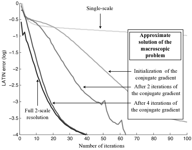
Figure 9: The LATIN convergence curves (error criterion vs. the number of iterations) for several numbers of macroiterations

5 Efficiency of the strategy: study of a complex test case

In this section, we illustrate the efficiency of the three-scale domain decomposition strategy through the simulation of the evolution of debonding in the bolted composite joint shown in Fig. 10. Each composite plate interacts with the adjacent plates and with the two steel bolts through contact interfaces. The structure is subjected to prescribed displacements along the edges of the plates.

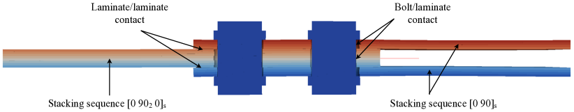
Figure 10: Composite bolted joint made of 16 $0.125$ mm-thick plies. The in-plane dimensions of the structure are $30\times 5$ mm. Prescribed displacements are applied along the left-hand side of the $[0\ 90_{2}\ 0]_{s}$ composite plate and along the right-hand sides of the $[0\ 90]_{s}$ composite plates.

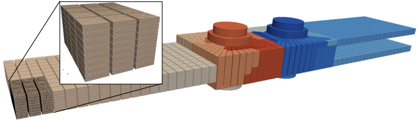
Figure 11: Discretization of the composite bolted joint ($12\,10^{6}$ DOFs), decomposition into substructures ($10,600$ substructures) and assignment to processors (29 CPUs)

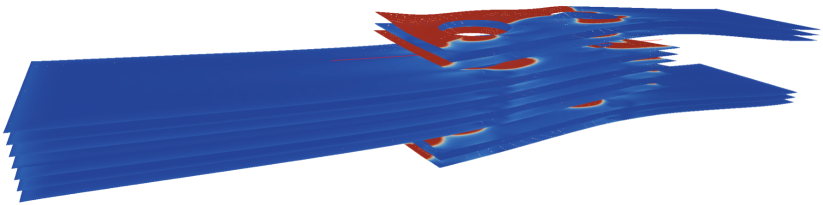
Figure 12: Damage map of the cohesive interfaces of the composite bolted joint after the 70${}^{\textrm{th}}$ time step of the quasi-static incremental analysis procedure

The discretization and the decomposition into substructures for this test case are illustrated in Fig. 11. The total number of DOFs involved was $12\,10^{6}$, distributed among $10,600$ substructures. The number of macroscopic DOFs was $3\,10^{5}$, which would have made the direct resolution on a standard computer very inefficient. 29 processors each with 4 Gigabytes memory were used for this calculation, which led to a super-coarse grid problem of dimension 150 (6 unknowns per floating super-substructure).

Figure 12 shows the damage map in the composite bolted joint after 70 time steps. The nonlinear calculation corresponding to each time step was carried out until the LATIN error criterion got below $10^{-2}$, which occurred after an average of $80$ LATIN iterations per time step. The average CPU time required for the calculation of each time step was 30 minutes, which is reasonable considering the small number of processors used.

However, the number of global LATIN iterations was quite high compared to what could have been obtained using the relocalization strategy of [11] in the vicinity of the crack’s front (see the results of Fig. 6). Figure 12 is a clear illustration of the difficulties which may arise in the use of this dedicated technique in a general case in which multiple crack front propagations may be involved. The front has a complex shape, which raises the difficult issue of the choice of the number of relocalization zones and their sizes. In addition, this test case is very unstable. These instabilities were handled globally using an arc-length algorithm along with the three-scale resolution strategy, but local instabilities might also appear within the region extracted for the relocalization calculations, a situation which has not yet been addressed at this stage in our development. Therefore, in the future, it might be necessary to generalize the relocalization strategy in order to improve the efficiency of the enhanced multiscale domain decomposition technique for complex laminated structures.

6 Conclusion

The accurate prediction of delamination in extended process zones of laminated composite structures requires refined models of the material’s behavior, leading to the resolution of huge systems of equations. In order to solve such problems accurately, we used a two-scale domain decomposition strategy based on an iterative resolution algorithm. This method is particularly appropriate for laminated mesomodels, in which 3D and 2D entities are introduced separately.

This strategy was improved in order to enable it to handle very large delamination problems. A systematic analysis of the features of the method on the different scales was performed. First, we showed that in the high-gradient zones the classical scale separation was insufficient to ensure numerical scalability. Therefore, we developed a subresolution procedure which preserves the numerical scalability of the crack propagation analysis, but still needs to be automated for complex structures and regulated against local instabilities. We also proved that a third scale is required. Then, the problem on the intermediate scale was solved using a parallel iterative algorithm which enabled the rapid transmission of the very-large-wavelength part of the solution. Global instabilities were handled through a classical arc-length algorithm with local control (e.g. based on the maximum damage increment) and adjustment of the “time” steps during the calculation of the evolution of damage.

In future developments, 3D analysis in the process zone will be used in conjunction with plate analysis, which would be sufficient to describe the solution in the low-gradient zones. We will also, within the MAAXIMUS project, investigate the interaction between delamination and buckling for the simulation of components of aeronautical structures.

References

- [1] O. Allix and P. Ladevèze. Interlaminar interface modelling for the prediction of delamination. Computers and structures, 22:235–242, 1992.
- [2] O. Allix, D. Lévèque, and L. Perret. Identification and forecast of delamination in composite laminates by an interlaminar interface model. Composites Science and Technology, 58:671–678, 1998.
- [3] R. De Borst and J. C. Remmers. Computational modelling of delamination. Composites Science and Technology, 66:713–722, 2006.
- [4] F. Feyel and J.-L. Chaboche. Fe2 multiscale approach for modelling the elastoviscoplastic behaviour of long fibre sic/ti composite materials. Computer Methods in Applied Mechanics and Engineering, 183:309–330, 2000.
- [5] J. Fish, K. Shek, M. Pandheeradi, and M. S. Shephard. Computational plasticity for composite structures based on mathematical homogenization: Theory and practice. Computer Methods in Applied Mechanics and Engineering, 148:53–73, 1997.
- [6] S. Ghosh, K. Lee, and P. Raghavan. A multi-level computational model for multi-scale damage analysis in composite and porous materials. International Journal of Solids and Structures, 38:2335–2385, 2001.
- [7] P. Gosselet and C. Rey. Non-overlapping domain decomposition methods in structural mechanics. Archives of Computational Methods in Engineering, 13:515–572, 2006.
- [8] D. Guedra Degeorges and P. Ladevèze, editors. Course on emerging techniques for damage prediction and failure analysis of laminated composite stuctures. Cepadues Editions, 2007.
- [9] T. Hettich, A. Hund, and E. Ramm. Modeling of failure in composites by x-fem and level sets within a multiscale framework. Computer Methods in Applied Mechanics and Engineering, 197(5):414–424, 2008.
- [10] T. J. R. Hughes, G. R. Feijoo, L. Mazzei, and J.-B. Quincy. The variarional multiscale—a paradigm for computational mechanics. Computer Methods in Applied Mechanics and Engineering, 166:3–24, 1998.
- [11] P. Kerfriden, O. Allix, and P. Gosselet. A three-scale domain decomposition method for the 3d analysis of debonding in laminates. Computational mechanics, 3(44):343–362, 2009.
- [12] P. Ladevèze. Multiscale modelling of damage and fracture processes in composite materials, chapter Multiscale computational damage modelling of laminate composites. Springer-Verlag, 2005.
- [13] P. Ladevèze and G. Lubineau. An enhanced mesomodel for laminates based on micromechanics. Composites Science and Technology, 62(4):533–541, 2002.
- [14] P. Ladevèze and A. Nouy. On a multiscale computational strategy with time and space homogenization for structural mechanics. Computer Methods in Applied Mechanics and Engineering, 192:3061–3087, 2003.
- [15] P. Le Tallec. Domain decomposition methods in computational mechanics. In Computational Mechanics Advances, volume 1. Elsevier, 1994.
- [16] G. Lubineau and P. Ladevèze. Construction of a micromechanics-based intralaminar mesomodel, and illustrations in abaqus/standard. Computational Materials Science, 43(17/18):137–145, 2008.
- [17] G. Lubineau, P. Ladevèze, and D. Marsal. Towards a bridge between the micro- and mesomechanics of delamination for laminated composites. Composites Science and Technology, 66(6):698–712, 2007.
- [18] G. Lubineau, D. Violeau, and P. Ladevèze. Illustrations of a microdamage model for laminates under oxidizing thermal cycling. Composites Science and Technology, 69(1):3–9, 2009.
- [19] J. Mandel. Balancing domain decomposition. Communications in Numerical Methods in Engineering, 9(233-241), 1993.
- [20] J. Melenk and I. Babuška. The partition of unity finite element method: basic theory and applications. Computer Methods in Applied Mechanics and Engineering, 39:289–314, 1996.
- [21] J. T. Oden, K. Vemaganti, and N. Moës. Hierarchical modeling of heterogeneous solids. Computer Methods in Applied Mechanics and Engineering, 172:3–25, 1999.
- [22] J.C.J. Schellekens and R. de Borst. Free edge delamination in carbon-epoxy laminates : a novel numerical/experimental approach. Composite structures, 28(4):357–373, 1994.