Accelerating Nesterov’s Method for Strongly Convex Functions with Lipschitz Gradient

Abstract

We modify Nesterov’s constant step gradient method for strongly convex functions with Lipschitz continuous gradient described in Nesterov’s book. Nesterov shows that $f(x_{k})-f^{*}\leq L\prod_{i=1}^{k}(1-\alpha_{k})\|x_{0}-x^{*}\|_{2}^{2}$ with $\alpha_{k}=\sqrt{\rho}$ for all $k$, where $L$ is the Lipschitz gradient constant and $\rho$ is the reciprocal condition number of $f(x)$. Hence the convergence rate is $1-\sqrt{\rho}$. In this work, we try to accelerate Nesterov’s method by adaptively searching for an $\alpha_{k}>\sqrt{\rho}$ at each iteration. The proposed method evaluates the gradient function at most twice per iteration and has some extra Level 1 BLAS operations. Theoretically, in the worst case, it takes the same number of iterations as Nesterov’s method does but doubles the gradient calls. However, in practice, the proposed method effectively accelerates the speed of convergence for many problems including a smoothed basis pursuit denoising problem.

1 Introduction

First-order methods for convex optimization have drawn great interest in recent years as the problem scale goes larger and larger. High-order methods do not fit the scene quite well because they generally need more memory than first-order methods and take many more operations per iteration. However, the slow convergence rate of first-order methods prevents them from practical use. For example, the constant step gradient descent method converges at the speed of $\mathcal{O}(1/k)$ for functions with Lipschitz gradient (with constant $L$), where $k$ is the number of iterations. It means that we need one million iterations to reach $f(x_{k})-f^{*}<\mathcal{O}(10^{-6})(f(x_{0})-f^{*})$. Nesterov [5] advanced the field with a first-order method converging at the speed of $\mathcal{O}(1/k^{2})$. We refer to this method as $\mathcal{N}_{L}$. To reach the same precision as in the previous example, $\mathcal{N}_{L}$ only needs one thousand iterations. Nesterov not only shows the method is faster than the gradient descent method but also shows that it is optimal among all first-order methods on functions with Lipschitz gradient. To seek a first-order method with higher-order convergence, we have to restrict the functions of interest. Nesterov [6] considered functions with both Lipschitz gradient and strong convexity (with parameter $\mu$), and he constructed another first-order method with linear convergence rate, referred to as $\mathcal{N}_{\mu,L}$. The gradient descent method can also achieve linear convergence on those functions. Nevertheless, to reach a given precision, the number of iterations the gradient descent method needs is $\mathcal{O}(\kappa)$, where $\kappa$ is the condition number of the objective function, while the number of iterations $\mathcal{N}_{\mu,L}$ needs is only $\mathcal{O}(\sqrt{\kappa})$, which is proved to be optimal too.

In this work, we are interested in accelerating $\mathcal{N}_{\mu,L}$ in a practical way. In section 2, we briefly review how Nesterov constructs $\mathcal{N}_{\mu,L}$. Then we present our modification to Nesterov’s method in section 3. Related work on improving Nesterov’s methods is discussed in section 4, and section 5 reports numerical results.

2 Nesterov’s method

We briefly review Nesterov’s constant step gradient method for strongly convex functions with Lipschitz gradient, referred to as $\mathcal{N}_{\mu,L}$, and its convergence properties. The content is mostly taken from Nesterov [6] with some simplifications. We keep this section short and concise but detail how Nesterov constructs the method because our modification is based on it. We begin with the definition of $S_{\mu,L}$, the class of strongly convex functions with Lipschitz gradient, and an assumption on first-order methods.

Definition 1.

A continuous differentiable function $f(x)$ is in $S_{\mu,L}(\Omega)$ for some $L\geq\mu>0$ if for any $x,y\in\Omega$ we have both of the following:

$$\|f^{\prime}(x)-f^{\prime}(y)\|_{2}\leq L\|x-y\|_{2},$$ (1)

$$f(y)\geq f(x)+\langle f^{\prime}(x),y-x\rangle+\frac{\mu}{2}\|y-x\|_{2}^{2}.$$ (2)

The value $\kappa=L/\mu$ is called the condition number of $f(x)$ and $\rho=1/\kappa$ is called the reciprocal condition number of $f(x)$.

Throughout, we assume that for a function from $S_{\mu,L}$ either $\mu$ and $L$ or a lower bound of $\mu$ and an upper bound of $L$ are given.

Assumption 2.1.

[6, p. 59] A first-order method generates a sequence of points $\{x_{k}\}$ such that $x_{k}\in x_{0}+\text{Span}\left\{f^{\prime}(x_{0}),\ldots,f^{\prime}(x_{k-1})\right\},k\geq 1.$

For functions in $S_{\mu,L}$, Nesterov constructs a first-order method, $\mathcal{N}_{\mu,L}$, and shows that it matches a lower complexity bound for first-order methods satisfying Assumption 2.1 up to a constant factor in the sense of worst-case number of iterations. Nesterov [6] gives more details on the optimality. Note that Assumption 2.1 is very mild, as most first-order methods fall into the framework, which secures the optimality of $\mathcal{N}_{\mu,L}$. To construct such an optimal first-order method, Nesterov introduces an estimate sequence and shows how it helps derive $\mathcal{N}_{\mu,L}$ and prove its convergence rate.

Definition 2.

[6, p. 72] A pair of sequences $\{\phi_{k}(x)\}$ and $\{\lambda_{k}\}$, $\lambda_{k}\geq 0$ is called an estimate sequence of $f(x)$ if $\lambda_{k}\to 0$ and we have

$$\phi_{k}(x)\leq(1-\lambda_{k})f(x)+\lambda_{k}\phi_{0}(x),\quad\forall x\in\mathbb{R}^{n}\text{ and }k\geq 0.$$ (3)

Lemma 3.

[6, p. 72] If the pair of sequences $\{\phi_{k}(x)\}$ and $\{\lambda_{k}\}$ is an estimate sequence of $f(x)$ and for some sequence $\{x_{k}\}$ we have

$$f(x_{k})\leq\phi_{k}^{*}\equiv\min_{x\in\mathbb{R}^{n}}\phi_{k}(x),$$ (4)

then $f(x_{k})-f^{*}\leq\lambda_{k}[\phi_{0}(x^{*})-f^{*}]\to 0$, where $x^{*}$ is the optimal value of $f(x)$.

Now the question becomes, given $f(x)\in S_{\mu,L}$, how can we construct an estimate sequence of $f(x)$ and generate a sequence $\{x_{k}\}$ satisfying (4). To construct an estimate sequence, we have the following lemma.

Lemma 4.

[6, p. 72] Assume the following:

1. $f\in S_{\mu,L}(\mathbb{R}^{n})$,

2. $\phi_{0}(x)$ is an arbitrary function on $\mathbb{R}^{n}$,

3. $\{y_{k}\}$ is an arbitrary sequence in $\mathbb{R}^{n}$,

4. $\{\alpha_{k}\}:\alpha_{k}\in(0,1)$, $\sum_{k=0}^{\infty}\alpha_{k}=\infty$,

5. $\lambda_{0}=1$.

Then the pair of sequences $\{\phi_{k}(x)\}$, $\{\lambda_{k}\}$ recursively defined by

$$\lambda_{k+1} = (1-\alpha_{k})\lambda_{k},$$ (5)

$$\phi_{k+1}(x) = (1-\alpha_{k})\phi_{k}(x)+\alpha_{k}\left[f(y_{k})+\langle f^{\prime}(y_{k}),x-y_{k}\rangle+\frac{\mu}{2}\|x-y_{k}\|_{2}^{2}\right],$$ (6)

is an estimate sequence.

We see that Lemma 4 leaves us freedom in the choice of $\phi_{0}(x)$, $\{y_{k}\}$, and $\{\alpha_{k}\}$. To combine the result from Lemma 3, we should choose a simple $\phi_{0}(x)$ such that $\phi_{k}^{*}$ is easy to obtain in explicit form, and choose $\{y_{k}\}$ and $\{\alpha_{k}\}$ appropriately such that we can find $x_{k}$ satisfying $f(x_{k})\leq\phi_{k}^{*}$ for each $k$. The following lemma is a simplified version of Lemma $2.2.3$ of Nesterov [6, p. 69].

Lemma 5.

Let $\phi_{0}(x)=\phi_{0}^{*}+\frac{\mu}{2}\|x-v_{0}\|_{2}^{2}$. Then the process defined in Lemma 4 preserves the canonical form of functions $\{\phi_{k}(x)\}$:

$$\phi_{k}(x)\equiv\phi_{k}^{*}+\frac{\mu}{2}\|x-v_{k}\|_{2}^{2},$$ (7)

where the sequences $\{v_{k}\}$ and $\{\phi_{k}^{*}\}$ are defined as follows:

$$v_{k+1} = (1-\alpha_{k})v_{k}+\alpha_{k}y_{k}-\frac{\alpha_{k}}{\mu}f^{\prime}(y_{k}),$$ (8)

$$\phi_{k+1}^{*} = (1-\alpha_{k})\phi_{k}^{*}+\alpha_{k}f(y_{k})-\frac{\alpha_{k}^{2}}{2\mu}\|f^{\prime}(y_{k})\|_{2}^{2}$$

$$\hbox{}+\alpha_{k}(1-\alpha_{k})\left(\frac{\mu}{2}\|y_{k}-v_{k}\|_{2}^{2}+\langle f^{\prime}(y_{k}),v_{k}-y_{k}\rangle\right).$$

Suppose we have $\phi_{k}^{*}\geq f(x_{k})$ at the $k$-th iteration. By (2) we know

$$\phi_{k}^{*}\geq f(y_{k})+\langle f^{\prime}(y_{k}),x_{k}-y_{k}\rangle+\frac{\mu}{2}\|x_{k}-y_{k}\|_{2}^{2}.$$

Plugging it into (5), we get

$$\phi_{k+1}^{*} \geq f(y_{k})-\frac{\alpha_{k}^{2}}{2\mu}\|f^{\prime}(y_{k})\|^{2}+(1-\alpha_{k})\langle f^{\prime}(y_{k}),\alpha_{k}(v_{k}-y_{k})+(x_{k}-y_{k})\rangle$$

$$\hbox{}+\frac{\mu(1-\alpha_{k})}{2}\left(\alpha_{k}\|v_{k}-y_{k}\|_{2}^{2}+\|x_{k}-y_{k}\|_{2}^{2}\right).$$

Remember that $y_{k}$ is arbitrary. We can choose $y_{k}=(x_{k}+\alpha_{k}v_{k})/(1+\alpha_{k})$ to eliminate the linear term associated with $f^{\prime}(y_{k})$ and drop the sum of squares. Then we have

$$\phi_{k+1}^{*}\geq f(y_{k})-\frac{\alpha_{k}^{2}}{2\mu}\|f^{\prime}(y_{k})\|_{2}^{2}.$$

Therefore, to make $\phi_{k+1}^{*}\geq f(x_{k+1})$, it is sufficient to find an $x_{k+1}$ such that

$$f(x_{k+1})\leq f(y_{k})-\frac{\alpha_{k}^{2}}{2\mu}\|f^{\prime}(y_{k})\|_{2}^{2}.$$

Because $f^{\prime}(x)$ is Lipschitz continuous with constant $L$, by choosing $x_{k+1}=y_{k}-\frac{1}{L}f^{\prime}(y_{k})$ we can always ensure

$$f(x_{k+1})\leq f(y_{k})-\frac{1}{2L}\|f^{\prime}(y_{k})\|_{2}^{2}.$$ (11)

Comparing the two inequalities above, we see setting $\alpha_{k}=\sqrt{\mu/L}=\sqrt{\rho}$ would suffice. Now we can further simplify the update scheme by knocking out $\{v_{k}\}$. We have

$$y_{k+1} = \frac{x_{k+1}+\alpha v_{k+1}}{1+\alpha}=\frac{x_{k+1}+\alpha\left[(1-\alpha)v_{k}+\alpha y_{k}-\frac{\alpha}{\mu}f^{\prime}(y_{k})\right]}{1+\alpha}$$

$$= \frac{x_{k+1}+\alpha\left[(1-\alpha)\frac{(1+\alpha)y_{k}-x_{k}}{\alpha}+\alpha y_{k}-\frac{\alpha}{\mu}f^{\prime}(y_{k})\right]}{1+\alpha}$$

$$= x_{k+1}+\frac{1-\alpha}{1+\alpha}(x_{k+1}-x_{k}).$$

We summarize this method in Algorithm 1, which is extremely simple. The term $\frac{1-\sqrt{\rho}}{1+\sqrt{\rho}}$ is called the acceleration parameter.

Algorithm 1 $\mathcal{N}_{\mu,L}$, Nesterov’s constant step scheme, III [6, p. 81]

1:  Given $f(x)\in S_{\mu,L}$ and $x_{0}$, set $\rho=\mu/L$ and $y_{0}=x_{0}$.

2:  for $k=0,1,\ldots$ until convergence do

3:     $x_{k+1}=y_{k}-\frac{1}{L}f^{\prime}(y_{k})$

4:     $y_{k+1}=x_{k+1}+\frac{1-\sqrt{\rho}}{1+\sqrt{\rho}}(x_{k+1}-x_{k})$

5:  end for

Let $\phi_{0}^{*}=f(x_{0})$, then Lemmas 3 and 4 characterize the convergence of $\mathcal{N}_{\mu,L}$. The following theorem is a simplified version of Theorem 2.2.3 of Nesterov [6, p. 80]:

Theorem 6.

$\mathcal{N}_{\mu,L}$ (Algorithm 1) generates a sequence $\{x_{k}\}$ such that

$$f(x_{k})-f^{*}\leq\left(1-\sqrt{\rho}\right)^{k}\left(f(x_{0})+\frac{\mu}{2}\|x_{0}-x^{*}\|_{2}^{2}-f^{*}\right)\leq L(1-\sqrt{\rho})^{k}\|x_{0}-x^{*}\|_{2}^{2}.$$ (12)

Note that Nesterov actually provides three variants in [6] and what we mentioned here is the third one. For the other two, $\{\alpha_{k}\}$ is not a constant sequence but deterministic and having $\alpha_{k}\to\sqrt{\rho}$ as $k\to\infty$; hence the asymptotic convergence rate is still $1-\sqrt{\rho}$. In practice, they perform quite similarly, while the third is the least expensive among the three variants.

3 Accelerating Nesterov’s method with adaptive $\alpha_{k}$

In $\mathcal{N}_{\mu,L}$, the rate of decrease of $f(x_{k})-f^{*}$ at the $k$-th iteration is bounded by $1-\alpha_{k}$, where $\alpha_{k}=\sqrt{\rho}$ for all $k$. Our modified method is based on the following idea: trying to make $\alpha_{k}$ larger than $\sqrt{\rho}$ at each iteration in order to accelerate the convergence. To see how it works, we need to revisit Nesterov’s construction, particularly the inequality (2). Given (2), it is sufficient to find $\alpha_{k}$, $y_{k}$, and $x_{k+1}$ such that

$$f(x_{k+1}) \leq f(y_{k})-\frac{\alpha_{k}^{2}}{2\mu}\|f^{\prime}(y_{k})\|_{2}^{2}$$

$$\hbox{}+(1-\alpha_{k})\langle f^{\prime}(y_{k}),\alpha_{k}(v_{k}-y_{k})+(x_{k}-y_{k})\rangle$$

$$\hbox{}+\frac{\mu(1-\alpha_{k})}{2}\left(\alpha_{k}\|v_{k}-y_{k}\|_{2}^{2}+\|x_{k}-y_{k}\|_{2}^{2}\right)$$

to retain (4): $f(x_{k+1})\leq\phi_{k+1}^{*}$. The goal of finding an $\alpha_{k}\in[0,1]$ as large as possible leads us to the following optimization problem:

maximize $$\alpha_{k}\in[0,1]$$

subject to $$f(x_{k+1})\leq f(y_{k})-\frac{\alpha_{k}^{2}}{2\mu}\|f^{\prime}(y_{k})\|_{2}^{2}$$

$$\hbox{}+(1-\alpha_{k})\langle f^{\prime}(y_{k}),\alpha_{k}(v_{k}-y_{k})+(x_{k}-y_{k})\rangle$$

$$\hbox{}+\frac{\mu(1-\alpha_{k})}{2}\left(\alpha_{k}\|v_{k}-y_{k}\|_{2}^{2}+\|x_{k}-y_{k}\|_{2}^{2}\right),$$

where $\alpha_{k}$, $y_{k}$, and $x_{k+1}$ are free variables, while $v_{k}$ is determined at step $k$. Apparently, one optimal solution is given by $\alpha_{k}^{*}=1$ and $x_{k+1}^{*}=y_{k}^{*}=x^{*}$. However, $x^{*}$ is unknown and $y_{k}$ and $x_{k+1}$ should be derived from past iterates and gradients. So we can only expect a sub-optimal solution that is good and easy to obtain. To restrict the optimization problem, we fix the choices of $y_{k}$ and $x_{k+1}$, following Nesterov:

$$y_{k}=\frac{x_{k}+\alpha_{k}v_{k}}{1+\alpha_{k}},\quad x_{k+1}=y_{k}-\frac{1}{L}f^{\prime}(y_{k}).$$ (14)

The choice of $y_{k}$ eliminates the linear term associated with $f^{\prime}(y_{k})$ and we have

$$\frac{\mu(1-\alpha_{k})}{2}\left(\alpha_{k}\|v_{k}-y_{k}\|_{2}^{2}+\|x_{k}-y_{k}\|_{2}^{2}\right)=\frac{\mu\alpha_{k}(1-\alpha_{k})}{2(1+\alpha_{k})}\|x_{k}-v_{k}\|_{2}^{2}.$$

Plugging (14) into (3), we get

maximize $$\alpha_{k}\in[0,1]$$

subject to $$f(x_{k+1})\leq f(y_{k})-\frac{\alpha_{k}^{2}}{2\mu}\|f^{\prime}(y_{k})\|_{2}^{2}+\frac{\mu\alpha_{k}(1-\alpha_{k})}{2(1+\alpha_{k})}\|x_{k}-v_{k}\|_{2}^{2}.$$ (15)

Since evaluating the function costs time, we would be better to eliminate $f(x_{k+1})$ and $f(y_{k})$ from the above inequality. Note that $f^{\prime}(x)$ is Lipschitz continuous and hence the choice of $x_{k+1}$ implies (11). Reinforcing the inequality (15) by (11), we get

maximize $$\alpha_{k}$$

subject to $$\left(\alpha_{k}^{2}-\rho\right)\left\|f^{\prime}\left(\frac{x_{k}+\alpha_{k}v_{k}}{1+\alpha_{k}}\right)\right\|_{2}^{2}\leq\mu^{2}\|x_{k}-v_{k}\|_{2}^{2}\frac{\alpha_{k}(1-\alpha_{k})}{1+\alpha_{k}},$$ (16)

where $\alpha_{k}\in[0,1]$ is implied by the constraint. Now $\alpha_{k}$ is the only free variable. The constraint always holds if $\alpha_{k}=\sqrt{\rho}$. Moreover, the constraint is not tight at $\alpha_{k}=\sqrt{\rho}$ if $x_{k}\neq v_{k}$, which is generally the case. So we can almost always expect an $\alpha_{k}>\sqrt{\rho}$ at each iteration. However, the problem is still nonlinear and solving it may lead to many function calls to the gradient function, which is inefficient because with those gradient calls we can proceed with the same number of iterations in $\mathcal{N}_{\mu,L}$. We try to solve this problem approximately with the hope of getting $\alpha_{k}$ as large as possible in one or two gradient calls. The idea is inspired by the following lemma.

Lemma 7.

Given $f(x)\in S_{\mu,L}$, let the pair of sequences $\{\phi_{k}(x)=\phi_{k}^{*}+\frac{\mu}{2}\|x-v_{k}\|_{2}^{2}\}$ and $\{\lambda_{k}\}$ be as defined in Lemmas 4 and 5. If for some sequence $\{x_{k}\}$ we have $f(x_{k})\leq\phi_{k}^{*}$ for all $k$, then $\lim_{k\to\infty}v_{k}=x^{*}$.

Proof.

The pair of sequences $\{\phi_{k}(x)\}$ and $\{\lambda_{k}\}$ is an estimate sequence. By definition we have

$$\phi_{k}(x^{*})\leq(1-\lambda_{k})f(x^{*})+\lambda_{k}\phi_{0}(x^{*}),\quad\forall k\geq 0,$$

and $\lim_{k\to\infty}\lambda_{k}=0$. Given $f(x^{*})\leq f(x_{k})\leq\phi_{k}^{*}$, we know

$$\frac{\mu}{2}\|v_{k}-x^{*}\|_{2}^{2}=\phi_{k}(x^{*})-\phi_{k}^{*}\leq(1-\lambda_{k})f(x^{*})+\lambda_{k}\phi_{0}(x^{*})-f(x^{*})=\lambda_{k}(\phi_{0}(x^{*})-f(x^{*})).$$

Letting $k\to\infty$ on both sides, we have $\lim_{k\to\infty}\|v_{k}-x^{*}\|_{2}^{2}=0$ and hence $\lim_{k\to\infty}v_{k}=x^{*}$. ∎

As long as $y_{k}$ is chosen as in (14), by Lemmas 3 and 7 we have $\lim_{k\to\infty}y_{k}=x^{*}$ and thus the global trend for $\|f^{\prime}(y_{k})\|_{2}$ is decreasing. So if assuming the change between two contiguous iterations is small, we can use $\|f^{\prime}(y_{k-1})\|_{2}$ as an approximate upper bound on $\|f^{\prime}(y_{k})\|_{2}$ to save the cost of evaluating gradients since $\|f^{\prime}(y_{k-1})\|_{2}$ is already calculated in the previous step. The modified constraint is therefore

$$\left(\alpha_{k}^{2}-\rho\right)\left\|f^{\prime}(y_{k-1})\right\|_{2}^{2}\leq\frac{\mu^{2}\alpha_{k}(1-\alpha_{k})}{1+\alpha_{k}}\|x_{k}-v_{k}\|_{2}^{2},$$ (17)

which is equivalent to

$$\alpha_{k}^{3}+(1+D_{k})\alpha_{k}^{2}-(\rho+D_{k})\alpha_{k}-\rho\leq 0,$$

where $D_{k}=\mu^{2}\|x_{k}-v_{k}\|_{2}^{2}/\|f^{\prime}(y_{k-1})\|_{2}^{2}$. Let’s consider how to pick an $\alpha_{k}$ at each step. Define

$$\eta_{k}(\alpha)=\alpha^{3}+(1+D_{k})\alpha^{2}-(\rho+D_{k})\alpha-\rho.$$

If $D_{k}=0$ ($x_{k}=v_{k}$), then the largest $\alpha$ satisfying $\eta_{k}(\alpha)\leq 0$ is $\sqrt{\rho}$. Assume that $D_{k}>0$ and $\rho<1$. It is easy to verify the following properties of $\eta_{k}(\alpha)$ by checking its first and second derivatives:

• $\eta_{k}(\alpha_{0})<0$, where $\alpha_{0}=\sqrt{\rho}$,

• $\eta_{k}(\alpha)$ has exactly one positive local minimum, denoted by $\beta_{k}$,

• $\eta_{k}(\alpha)$ has exactly one positive root, denoted by $\gamma_{k}$.

Fig. 1: Choosing $\alpha_{k}$: 1) $\alpha_{k}=\alpha_{0}=\sqrt{\rho}$, we always have $\eta_{k}(\alpha_{0})\leq 0$, 2) $\alpha_{k}=\gamma_{k}$, the positive root of $\eta_{k}(\alpha)$, is an aggressive choice because we don’t always have $\|f^{\prime}(y_{k-1})\|_{2}\geq\|f^{\prime}(y_{k})\|_{2}$, 3) $\alpha_{k}=\beta_{k}$, the local minimum of $\eta_{k}(\alpha)$, is a generally safe choice if $\beta_{k}>\alpha_{0}$.

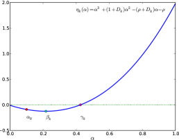
Figure 1 shows a typical plot of $\eta_{k}(\alpha)$ with $\alpha_{0}$, $\beta_{k}$, and $\gamma_{k}$. Note that $\beta_{k}$ is not necessarily larger than $\alpha_{0}$. Choosing $\alpha_{k}=\alpha_{0}$ always leads to a valid estimate sequence that guarantees convergence. Given $\alpha_{0}$ as our fallback choice, we try to be more aggressive. $\alpha_{k}=\gamma_{k}$ is apparently the most aggressive choice. However, if we choose $\alpha_{k}=\gamma_{k}$, (3) may break frequently because $\|f^{\prime}(y_{k-1})\|_{2}$ is not always an upper bound on $\|f^{\prime}(y_{k})\|_{2}$. If $\beta_{k}>\alpha_{0}$, $\alpha_{k}=\beta_{k}$ may be a safe choice that is more robust to the violation of $\|f^{\prime}(y_{k-1})\|_{2}\geq\|f^{\prime}(y_{k})\|_{2}$. Based on these observations, we propose four heuristics (from conservative to aggressive) to pick an $\alpha_{k}$ and compare their performance later in section 5. They are as follows:

1. $\alpha_{k}=\max(\alpha_{0},\beta_{k})$,

2. $\alpha_{k}=\frac{1}{2}(\alpha_{0}+\gamma_{k})$,

3. $\alpha_{k}=\frac{1}{2}(\max(\alpha_{0},\beta_{k})+\gamma_{k})$.

4. $\alpha_{k}=\gamma_{k}$.

As mentioned before, having an $\alpha_{k}$ satisfying constraint (17) doesn’t imply that $\alpha_{k}$ is feasible in (3). If our guess doesn’t meet the constraint, we fall back to Nesterov’s choice $\alpha_{k}=\sqrt{\rho}$ without making extra effort in searching for an $\alpha_{k}>\sqrt{\rho}$. Therefore, the modified method calls the gradient function at most twice per iteration and has at least the same rate of convergence as $\mathcal{N}_{\mu,L}$ in terms of number of iterations.

We summarize our modified method in Algorithm 2 and refer to it as $\mathcal{N}_{\mu,L}^{\alpha}$. To differentiate the four heuristics we proposed to pick an $\alpha_{k}$, we call the corresponding variants $\mathcal{N}_{\mu,L}^{\alpha,1}$, $\mathcal{N}_{\mu,L}^{\alpha,2}$, $\mathcal{N}_{\mu,L}^{\alpha,3}$, and $\mathcal{N}_{\mu,L}^{\alpha,4}$, respectively.

Algorithm 2 $\mathcal{N}_{\mu,L}^{\alpha}$, Nesterov’s constant step scheme with adaptive $\alpha_{k}$

1:  Given $f(x)\in S_{\mu,L}(\mathbb{R}^{n})$ and $x_{0}$, set $v_{0}=y_{0}=x_{0}$ and $\alpha_{0}=\sqrt{\rho}=\sqrt{\mu/L}$.

2:  Compute $x_{1}=y_{0}-\frac{1}{L}f^{\prime}(y_{0})$.

3:  for $k=1,2,\ldots$ until convergence do

4:     Compute $v_{k}=(1-\alpha_{k-1})v_{k-1}+\alpha_{k-1}y_{k-1}-\frac{\alpha_{k-1}}{\mu}f^{\prime}(y_{k-1})$.

5:     Let $D_{k}=\mu^{2}\|x_{k}-v_{k}\|_{2}^{2}/\|f^{\prime}(y_{k-1})\|_{2}^{2}$. Choose an $\tilde{\alpha}_{k}\geq\sqrt{\rho}$ such that

$$\tilde{\alpha}_{k}^{3}+(1+D_{k})\tilde{\alpha}_{k}^{2}-(\rho+D_{k})\tilde{\alpha}_{k}-\rho\leq 0.$$

6:     Compute $\tilde{y}_{k}=(x_{k}+\tilde{\alpha}_{k}v_{k})/(1+\tilde{\alpha}_{k})$ and $\tilde{x}_{k+1}=\tilde{y}_{k}-\frac{1}{L}f^{\prime}(\tilde{y}_{k})$.

7:     Validate whether we have $f(\tilde{x}_{k+1})\leq\phi_{k+1}^{*}$ by verifying a more stringent inequality

$$(\tilde{\alpha}_{k}^{2}-\rho)\|f^{\prime}(\tilde{y}_{k})\|_{2}^{2}\leq\mu^{2}\|x_{k}-v_{k}\|_{2}^{2}\frac{\tilde{\alpha}_{k}(1-\tilde{\alpha}_{k})}{1+\tilde{\alpha}_{k}}.$$

8:     If valid, let $\alpha_{k}=\tilde{\alpha}_{k}$, $y_{k}=\tilde{y_{k}}$, and $x_{k+1}=\tilde{x}_{k+1}$.Otherwise, let $\alpha_{k}=\sqrt{\rho}$, $y_{k}=(x_{k}+\alpha_{k}v_{k})/(1+\alpha_{k})$, and $x_{k+1}=y_{k}-\frac{1}{L}f^{\prime}(y_{k})$.

9:  end for

4 Related work

In this section, we discuss related work on accelerating Nesterov’s methods $\mathcal{N}_{L}$ and $\mathcal{N}_{\mu,L}$. In both $\mathcal{N}_{L}$ and $\mathcal{N}_{\mu,L}$, the global Lipschitz constant $L$ is assumed to be known. However, $L$ might be difficult to get, and even if $L$ is given, local Lipschitz constants may be much smaller than $L$ such that the step size $\frac{1}{L}$ becomes too conservative. A widely adopted solution is backtracking linesearch, where the step size is adaptively chosen. Tseng [10] presented a sufficient condition on the step size to preserve the convergence rate of $\mathcal{N}_{L}$. Becker et al. [1, §5.3] proposed an alternative condition that is numerically more stable to verify, and they also discussed implementation issues. Gonzaga and Karas [3] developed a linesearch scheme that preserves the convergence rate of $\mathcal{N}_{\mu,L}$ when only $\mu$ is given. Linesearch schemes generally do not need explicit knowledge of $L$, but a single search may require evaluating the objective function for several times. Hence, even if $L$ is provided, it is still problem-dependent whether we should use the constant step $\mathcal{N}_{L}$/$\mathcal{N}_{\mu,L}$ or a backtracking linesearch.

On strongly convex functions with Lipschitz gradient, $\mathcal{N}_{L}$ may converge at a rate $\mathcal{O}(1/k^{2})$ while even the steepest gradient descent method has linear convergence. Note that the optimal method $\mathcal{N}_{\mu,L}$ takes the same form as $\mathcal{N}_{L}$. The only difference is the acceleration parameter. $\mathcal{N}_{L}$ increases the acceleration parameter gradually. $\mathcal{N}_{\mu,L}$, given the global convexity parameter $\mu$, sets the acceleration parameter to a constant that guarantees linear convergence at an optimal rate. However, $\mu$ is not always known. Nesterov [8] proposed a practical approach to discover strong convexity: restarting $\mathcal{N}_{L}$ after a certain number of iterations. Theoretically, whether we should restart $\mathcal{N}_{L}$ depends on the local condition number. Empirically, even with sub-optimal choices, linear convergence rate can be achieved. See Becker et al. [1, §5.6] for more details. Gonzaga and Karas [3] developed an adaptive procedure to estimate $\mu$ at the cost of function evaluations.

In this work, we assume that both $\mu$ and $L$ are given and only the gradient function is used to maintain minimal cost per iteration. We save gradient calls based on the global trend of $\|f^{\prime}(y_{k})\|_{2}$. We argue that there are many cases where $\mu$ and $L$ are easy to obtain. $L$ can be easily estimated for a quadratic function, or derived from a smooth approximation of a non-smooth function [7], and $\mu$ can be derived from a quadratic regularization term, e.g., $\frac{\mu}{2}\|x-c\|^{2}$, or by adding a quadratic term to the objective manually and then performing sequential updates.

5 Numerical experiments

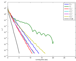
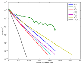
We compare the four variants of $\mathcal{N}_{\mu,L}^{\alpha}$ with $\mathcal{N}_{L}$ and $\mathcal{N}_{\mu,L}$. We implement $\mathcal{N}_{\mu,L}^{\alpha}$ in MATLAB. The source code is available for download together with code that can be used to reproduce our results. $\mathcal{N}_{L}$ doesn’t take $\mu$ as input and converges with rate $\mathcal{O}(1/k^{2})$. To recover linear convergence, as suggested by Nesterov [8] and Becker et al. [1], we restart $\mathcal{N}_{L}$ after a certain number of iterations. The optimal number of iterations between restarts is problem-dependent. For each test, we restart $\mathcal{N}_{L}$ every 10, 100, and 1000 iterations respectively, compare the convergence rates with $\mathcal{N}_{L}$ without restart, and present the best result. The experiments were performed on a laptop that has two Intel Core Duo CPU cores at clock rate 2.0GHz and 4GB RAM. Only one core was used to remove the effect of multi-threading. We compare the convergence based on number of gradient calls and on running times, rather than on number of iterations, because Nesterov’s methods call the gradient function exactly once per iteration, but $\mathcal{N}_{\mu,L}^{\alpha}$ may call the gradient function twice per iteration. The running times were measured in wall-clock times.

5.1 Ridge regression

Fig. 2: On a ridge regression problem. Top left: $f-f^{*}$ vs. number of gradient calls. Top right: $f-f^{*}$ vs. running time. Bottom left: $\|x-x^{*}\|_{2}$ vs. number of gradient calls. Bottom right: $\|x-x^{*}\|_{2}$ vs. running time. In terms of convergence speed, we have $\text{LSQR}>\mathcal{N}_{\mu,L}^{\alpha,1}>\mathcal{N}_{\mu,L}^{\alpha,2}>\mathcal{N}_{\mu,L}^{\alpha,3}>\mathcal{N}_{\mu,L}>\mathcal{N}_{\mu,L}^{\alpha,4}>\mathcal{N}_{L}$. $\mathcal{N}_{\mu,L}^{\alpha,4}$ is too aggressive and should be used with caution.

Our first test is on a ridge regression problem, i.e., a linear least squares problem with Tikhonov regularization:

$$\text{minimize}\quad f(x)=\frac{1}{2}\|Ax-b\|_{2}^{2}+\frac{\lambda}{2}\|x\|_{2}^{2},$$

where $A\in\mathbb{R}^{m\times n}$ is the measurement matrix, $b\in\mathbb{R}^{m}$ is the response vector, and $\lambda>0$ is the ridge parameter. The unique solution is given by $x^{*}=(A^{T}A+\lambda I)^{-1}A^{T}b$.

$f(x)$ is a positive definite quadratic function, the simplest function type in the $S_{\mu,L}$ family. $f(x)$ has Lipschitz gradient with constant $L=\|A\|_{2}^{2}+\lambda$ and strong convexity with parameter $\mu=\lambda$. It is easy to show that $\mathcal{N}_{\mu,L}$ automatically achieves better convergence rate on positive definite quadratic functions by exploring the eigenspace. We have

$$\|x_{k}-x^{*}\|_{2}\leq C_{0}\left(1-\sqrt{\rho}\right)^{k}\|x_{0}-x^{*}\|_{2}$$

for some constant $C_{0}>0$ and hence

$$f(x_{k})-f^{*}\leq\frac{L}{2}\|x_{k}-x^{*}\|_{2}^{2}\leq\frac{C_{0}^{2}L}{2}(1-\sqrt{\rho})^{2k}\|x_{0}-x^{*}\|_{2}^{2}.$$

We omit the proof because it is purely mechanic work. Another important fact about positive definite quadratic functions is that there exist algorithms that can achieve the lower complexity bound derived by Nesterov [6, p. 68], e.g., the conjugate gradient (CG) method. We refer readers to Luenberger [4] for a detailed analysis of CG’s convergence rate. For least squares problems, LSQR [9] is preferable because LSQR is equivalent to applying CG to the normal equation in exact arithmetic but numerically more stable. The purpose of this test is not to compete with LSQR, which is specifically designed to solve least squares problems, but to treat LSQR as an ideal method and see how $\mathcal{N}_{\mu,L}^{\alpha}$ can reduce the gap between $\mathcal{N}_{\mu,L}$ and the ideal method on the simplest function family in $S_{\mu,L}$.

We choose $m=1200$, $n=2000$, and $\lambda=1.0$. We generate $A$ from $U\Sigma V^{T}$ where $U\in\mathbb{R}^{m\times m}$ and $V\in\mathbb{R}^{n\times m}$ are orthonormal matrices chosen at random, $\Sigma\in\mathbb{R}^{m\times m}$ is a diagonal matrix with diagonal elements linearly spaced between and including $100$ and $1$. $b=\text{randn}(m,1)$ is a random vector whose entries are i.i.d. samples drawn from the standard normal distribution. Although the exact value is known, $\|A\|_{2}^{2}$ is estimated by applying the power method to $AA^{T}$. We have $\mu=1$ and $L\approx 10001$. Figure 2 shows the comparison results. LSQR leads as expected. $\mathcal{N}_{\mu,L}^{\alpha,1}$, $\mathcal{N}_{\mu,L}^{\alpha,2}$, and $\mathcal{N}_{\mu,L}^{\alpha,3}$ form the second group with $\mathcal{N}_{\mu,L}^{\alpha,1}$ having a slight edge. $\mathcal{N}_{\mu,L}^{\alpha,4}$ falls behind all other variants of $\mathcal{N}_{\mu,L}^{\alpha}$ and $\mathcal{N}_{\mu,L}$ because it is too aggressive on choosing an $\alpha_{k}$ and falls back to $\alpha_{k}=\sqrt{\rho}$ frequently. Hence $\mathcal{N}_{\mu,L}^{\alpha,4}$ should be used with caution. $\mathcal{N}_{L}$, even with restart, is the slowest among competitive methods. We see $\mathcal{N}_{\mu,L}^{\alpha,1}$ approximately reduces the gap between $\mathcal{N}_{\mu,L}$ and LSQR by a factor of $30\%$ in terms of number of gradient calls.

Anisotropic bowl

Fig. 3: On an anisotropic bowl. Top left: $f-f^{*}$ vs. number of gradient calls. Top right: $f-f^{*}$ vs. running time. Bottom left: $\|x-x^{*}\|_{2}$ vs. number of gradient calls. Bottom right: $\|x-x^{*}\|_{2}$ vs. running time. All the variants of $\mathcal{N}_{\mu,L}^{\alpha}$ converge significantly faster than $\mathcal{N}_{\mu,L}$ or $\mathcal{N}_{L}$.

The second test is on a bowl-shaped function, which is anisotropic along different directions:

minimize $$f(x)=\sum_{i=1}^{n}i\cdot x_{(i)}^{4}+\frac{1}{2}\|x\|_{2}^{2}$$

subject to $$\|x\|_{2}\leq\tau,$$

where we use $x_{(i)}$ to indicate the $i$-th element of $x$. We put a constraint to make $f(x)$ have a Lipschitz continuous gradient over the feasible region. If $x_{k}$ falls outside the feasible region, we project it back to the nearest feasible point. By doing so, we know the function value will be decreased, so the convergence result still holds. We use this example to test the performance of $\mathcal{N}_{\mu,L}^{\alpha}$ and competitive methods when the gradient has local Lipschitz constants that are much smaller than the global one.

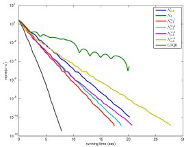
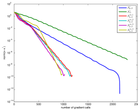
We choose $n=500$, $\tau=4$, and $x_{0}=\frac{\tau}{\sqrt{n}}\mathbf{1}$. With these choices, we have $L=12n\tau^{2}+1=96001$ and $\mu=1$. Figure 3 draws the convergence results. We see that all the variants of $\mathcal{N}_{\mu,L}^{\alpha}$ converge significantly faster than $\mathcal{N}_{\mu,L}$ or $\mathcal{N}_{L}$. For example, to reach $f(x_{k})-f^{*}<10^{-12}$, variants of $\mathcal{N}_{\mu,L}^{\alpha,1}$ take about $200$ gradient calls, $\mathcal{N}_{\mu,L}$ takes $5500$ gradient calls, and $\mathcal{N}_{L}$ takes $7000$ gradient calls. The differences among the four variants of $\mathcal{N}_{\mu,L}^{\alpha}$ are really small.

Fig. 4: Projected trajectory of $\{x_{k}\}$ on the plane spanned by $x_{(1)}$ and $x_{(n)}$. $\mathcal{N}_{\mu,L}$ and $\mathcal{N}_{\mu,L}^{\alpha}$ are almost following the same path, though $\mathcal{N}_{\mu,L}$ makes little progress per step, while $\mathcal{N}_{\mu,L}^{\alpha}$ has many large steps. We say $\mathcal{N}_{\mu,L}^{\alpha}$ accelerates $\mathcal{N}_{\mu,L}$ in this sense.

To investigate further, we plot the projected trajectory of $\{x_{k}\}$ on the plane spanned by $x_{(1)}$ and $x_{(n)}$ for each method. In Figure 4 we see that the point sequences generated by $\mathcal{N}_{\mu,L}^{\alpha}$ and $\mathcal{N}_{\mu,L}$ are almost following the same path. However, $\mathcal{N}_{\mu,L}$ makes very little progress per step, while $\mathcal{N}_{\mu,L}^{\alpha}$ jumps along the path. In this sense we say $\mathcal{N}_{\mu,L}^{\alpha}$ is indeed accelerating $\mathcal{N}_{\mu,L}$.

Smooth-BPDN

The third test is on a smoothed and strongly convex version of the basis pursuit denoising (BPDN) problem of Chen et al. [2]:

$$\text{minimize}\quad f(x)=\frac{1}{2}\|Ax-b\|_{2}^{2}+\lambda\|x\|_{\ell_{1},\tau}+\frac{\rho}{2}\|x\|_{2}^{2},$$

where $\|\cdot\|_{\ell_{1},\tau}$ is given by

$$\|x\|_{\ell_{1},\tau}=\begin{cases}|x|-\frac{\tau}{2}&\text{if }|x|\geq\tau\\ \frac{1}{2\tau}x^{2}&\text{if }|x|<\tau\end{cases}$$

if $x$ is a scalar and $\|x\|_{\ell_{1},\tau}=\sum_{i=1}^{n}\|x_{(i)}\|_{\ell_{1},\tau}$ if $x$ is a vector in $\mathbb{R}^{n}$. $\|\cdot\|_{\ell_{1},\tau}$ is a smoothed version of the $\ell_{1}$ norm, also recognized as the Huber penalty function with half-width $\tau$. $\lambda>0$ and $\rho>0$ are parameters controlling the penalty terms. The quadratic term $\frac{\rho}{2}\|x\|_{2}^{2}$ makes the function strongly convex. $f(x)$ has Lipschitz gradient with constant $L=\|A\|_{2}^{2}+\frac{\lambda}{\tau}+\rho$ and strong convexity with parameter $\mu=\rho$.

We set $A=\frac{1}{\sqrt{n}}\cdot\text{randn}(m,n)$, where $m=800$ and $n=2000$, $\lambda=0.05$, $\tau=0.0001$, and $\mu=0.05$. The true signal is a random sparse vector with $40$ nonzeros. $b=Ax^{*}+e$, where $e=0.01\frac{\|b\|_{2}}{\sqrt{m}}\cdot\text{randn}(m,1)$ is a Gaussian noise. $\|A\|_{2}^{2}$ is estimated by applying the power method to $AA^{T}$. The value is around $1.63$. Hence we have

$$L=\|A\|_{2}^{2}+\frac{\lambda}{\tau}+\rho\approx 502.7\text{ and }\mu=0.05.$$

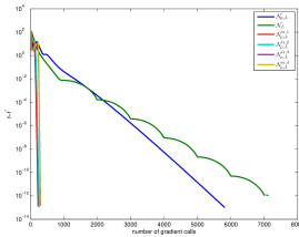
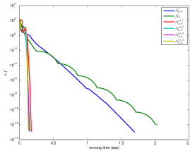
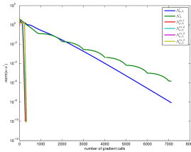
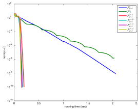
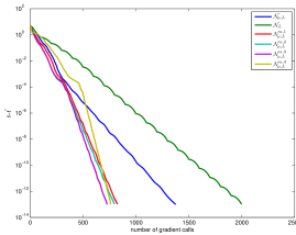
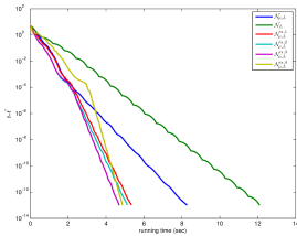
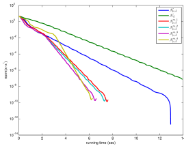
There is no analytic solution for this problem. We apply $\mathcal{N}_{\mu,L}$ to the problem with a small tolerance on the gradient norm and use the approximate solution returned by $\mathcal{N}_{\mu,L}$ as the optimal solution. Figure 5 presents the results. All variants of $\mathcal{N}_{\mu,L}^{\alpha}$ run faster than $\mathcal{N}_{\mu,L}$ or $\mathcal{N}_{L}$. It takes about $750$ gradient calls for $\mathcal{N}_{\mu,L}^{\alpha}$ to reach $f(x_{k})-f^{*}<10^{-12}$, $1300$ for $\mathcal{N}_{\mu,L}$, and $1900$ for $\mathcal{N}_{L}$. The corresponding running times are around $5$, $7.5$, and $11.5$ seconds, respectively. $\mathcal{N}_{\mu,L}^{\alpha,4}$ is slow at the beginning but becomes the fastest method at the end. However, the differences among the four variants of $\mathcal{N}_{\mu,L}^{\alpha}$ are not big.

Fig. 5: Smooth-BPDN. Top left: $f-f^{*}$ vs. number of gradient calls. Top right: $f-f^{*}$ vs. running time. Bottom left: $\|x-x^{*}\|_{2}$ vs. number of gradient calls. Bottom right: $\|x-x^{*}\|_{2}$ vs. running time. All the variants of $\mathcal{N}_{\mu,L}^{\alpha}$ converge faster than $\mathcal{N}_{\mu,L}$ or $\mathcal{N}_{L}$.

Fig. 6: Exact signal vs. smooth-BPDN solution. The smooth-BPDN solution is very close to a soft-thresholded version of the exact signal. Smooth-BPDN solution recovers all the coefficients with large magnitude.

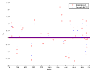
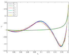
Though the purpose of this test is not to recover sparse signals but to compare $N_{\mu,L}^{\alpha}$ with competitive methods, we show that smooth-BPDN does recover sparse signals and hence it has practical value as well. Figure 6 compares the smooth-BPDN solution with the exact signal. We see the smooth-BPDN solution is very similar to a soft-thresholded version of the exact signal. It recovers all the coefficients with large magnitude.

In summary, the proposed method $\mathcal{N}_{\mu,L}^{\alpha}$ can effectively accelerate Nesterov’s method $\mathcal{N}_{\mu,L}$ in all the tests we present. Among the four variants, the first, second, and the third perform quite similarly. The fourth, the most aggressive one, may fall back frequently, as we see in the ridge regression case. Though it is the fastest method in the smooth-BPDN test, we don’t recommend it in general. Since the first heuristic is the most conservative one and delivers comparable performance in all the three tests, we suggest using $\mathcal{N}_{\mu,L}^{\alpha,1}$ as the default setting.

6 Conclusion and future work

We modified Nesterov’s constant step gradient method for strongly convex functions with Lipschitz gradient such that, at each iteration, we try to choose an $\alpha_{k}>\sqrt{\rho}$ adaptively while preserving the estimate sequence, where $\alpha_{k}$ controls the rate of decrease. $\mathcal{N}_{\mu,L}^{\alpha}$, the modified method, has at least the same convergence speed as Nesterov’s method. Though it may evaluate the gradient function twice per iteration, in practice it effectively accelerates the speed of convergence for many problems. We propose four heuristics for choosing $\alpha_{k}$, compare their performance in the numerical experiments, and suggest a default one to use.

Note that we don’t utilize all the degrees of freedom in constructing our method. The sequences $\{y_{k}\}$ and $\{x_{k}\}$ are still following Nesterov’s, so that we can reduce the number of calls to the gradient function. However, further exploration on the choices of $\{y_{k}\}$, $\{x_{k}\}$, and $\{\alpha_{k}\}$ may help discover more efficient methods or help design variable step size methods. We leave those possible directions as our future work.

The authors would like to thank Michael A. Saunders for useful comments on a previous draft of this paper.

References

- [1] S. R. Becker, E. J. Candès, and M. C. Grant, Templates for convex cone problems with applications to sparse signal recovery, Math. Prog. Comp., 3 (2011), pp. 165–218.
- [2] S. S. Chen, D. L. Donoho, and M. A. Saunders, Atomic decomposition by basis pursuit, SIAM J. Sci. Comput., 20 (1998), pp. 33–61.
- [3] C. C. Gonzaga and E. W. Karas, Fine tuning Nesterov’s steepest descent algorithm for differentiable convex programming, tech. report, Federal University of Paraná, Brazil, 2008.
- [4] D. G. Luenberger, Introduction to Linear and Nonlinear Programming, Addison-Wesley, 1973.
- [5] Y. Nesterov, A method of solving a convex programming problem with convergence rate , Soviet Math. Dokl., 27 (1983), pp. 372–376.
- [6] , Introductory Lectures on Convex Optimization: a Basic Course, Springer, 2003.
- [7] , Smooth minimization of non-smooth functions, Math. Program., 103 (2005), pp. 127–152.
- [8] , Gradient methods for minimizing composite objective function, tech. report, Center for Operations Research and Econometrics (CORE), Université Catholique de Louvain, 2007.
- [9] C. C. Paige and M. A. Saunders, LSQR: An algorithm for sparse linear equations and sparse least squares, ACM Trans. Math. Softw., 8 (1982), pp. 43–71.
- [10] P. Tseng, On accelerated proximal gradient methods for convex-concave optimization, submitted to SIAM J. Optim., (2008).